Abstract
Bank fraud detection faces critical challenges in imbalanced datasets, where fraudulent transactions are rare, severely impairing model generalization. This study proposes a Gaussian noise-based augmentation method to address class imbalance, contrasting it with SMOTE and ADASYN. By injecting controlled perturbations into the minority class, our approach mitigates overfitting risks inherent in interpolation-based techniques. Five classifiers, including XGBoost and a convolutional neural network (CNN), were evaluated on augmented datasets. XGBoost achieved superior performance with Gaussian noise-augmented data (accuracy: 0.999507, AUC: 0.999506), outperforming SMOTE and ADASYN. These results underscore Gaussian noise’s efficacy in enhancing fraud detection accuracy, offering a robust alternative to conventional oversampling methods. Our findings emphasize the pivotal role of augmentation strategies in optimizing classifier performance for imbalanced financial data.
1. Introduction
Nowadays, access to banking services and resources that were previously carried out in person, such as paying for a service, making deposits, and transferring money, among others, can now be done from anywhere in the world. All it takes is a device with internet access to perform any type of financial operation. As a result, electronic banking and financial transactions have become the primary activity of financial institutions in any global economy [1]. However, the risk of bank fraud has also increased, leading to significant financial losses for both customers and financial institutions [2,3,4].
Bank fraud represents any type of illegal activity carried out by internal bank employees, individuals, or external groups to gain access to customers’ confidential data [5]. These data can be used to impersonate their identities and steal the customers’ money. The most common types of electronic fraud include security breaches, data leaks, malware implantation, and fraud schemes, among others. In this context, one of the largest banks in Peru, Interbank, was a victim of a data breach by a third party, compromising the security of its customers’ data [6].
To mitigate malicious activities and protect users from potential fraud or cyberattacks, one of the main mechanisms that financial institutions have adopted in recent years is the constant and thorough monitoring of the digital transactions performed by users [7]. This process, carried out in real-time, is complemented by a combination of advanced machine learning techniques and algorithms, which allow for the identification of unusual or discrepant patterns in users’ transaction behaviors [8,9]. These analysis methods not only focus on identifying evident fraudulent activities but are also capable of recognizing atypical behaviors that could go unnoticed in traditional monitoring.
Despite the growing popularity of machine learning in financial decision-making due to its ability to make more accurate predictions, it still faces significant challenges. One of the main obstacles arises when models encounter imbalanced datasets, which hinder the correct representation of the minority class. This data imbalance can lead to unexpected behaviors and negatively impact the results obtained across various performance metrics [10,11]. This issue becomes more evident in datasets published regarding the study topic, where the minority class does not exceed 20% of the total data [12,13,14].
To address the data imbalance problem in the financial sector, techniques have been implemented to generate synthetic data that increase the size of the minority class, considered as the number of fraudulent transactions in relation to the majority class, which encompasses the number of normal transactions [11,15,16,17,18]. In other research analyzed, fraud detection has been approached without considering the data imbalance issue or it is not adequately described [8,19,20]. Other studies that have used oversampling techniques, such as Synthetic Minority Oversampling Technique (SMOTE), Adaptive Synthetic Sampling (ADASYN), and Random Undersampling (RUS), have not properly analyzed the risks associated with these techniques when generating duplicate data [16,21,22,23]. Hybrid methods that combine oversampling techniques implemented with other algorithms also fail to evaluate the duplicate values [24,25]. Therefore, training models with duplicate data is not recommended, as it can lead to model overfitting, which reduces performance when facing unseen or invisible data during the classification process [26].
This study proposes a novel methodology to address data imbalance in bank fraud detection through Gaussian noise-based augmentation. Traditional oversampling techniques like SMOTE and ADASYN, which generate synthetic samples via interpolation between existing data points, risk introducing artificial patterns that misrepresent the minority class. In fraud detection contexts, where subtle and non-linear transaction anomalies define fraudulent behavior, such interpolation can distort feature distributions, exacerbating overfitting and reducing model generalizability to unseen data. In contrast, our approach injects controlled perturbations into minority-class samples using Gaussian noise, enhancing dataset diversity while preserving the statistical integrity of the original data distribution. By avoiding synthetic data artifacts, this method mitigates overfitting risks inherent to SMOTE and ADASYN. Five classifiers, including a convolutional neural network (CNN), were evaluated on augmented datasets using eight metrics (e.g., AUC, MCC, G-Mean). Results demonstrate that XGBoost achieves superior accuracy (0.9995) with Gaussian noise-augmented data, outperforming conventional techniques. This underscores the method’s potential to balance class representation without compromising data authenticity, a critical advantage for real-world fraud detection systems.
The contributions of this work are threefold, a systematic comparison of Gaussian noise against SMOTE and ADASYN in fraud detection, empirical validation of noise-augmented data in improving classifier generalizability, and actionable insights into optimizing imbalance mitigation strategies for financial datasets. These advancements bridge a critical gap in ML-driven fraud detection, where synthetic data quality directly impacts model reliability.
The remainder of this paper is structured as follows: Section 2 details the methodology, including data augmentation and classifier configurations. Section 3 presents the experimental results, followed by a discussion of their implications. Finally, conclusions and future research directions are outlined in Section 4.
2. Materials and Methods
The methodology, shown in Figure 1, begins with the identification of the bank fraud dataset, where all records and features underwent data cleaning to remove empty values, duplicates, and features with zero variance. Next, the dataset was split into 80% for training, 10% for validation, and 10% for testing. In the training subset, data augmentation techniques were applied to balance the minority class with the majority class. For optimal hyperparameter selection, a cross-validation procedure (cv = 10) was implemented to improve the model’s generalization capacity. The optimal model (best model), after validation, was then evaluated using the testing set to measure the performance of the ML and DL models.
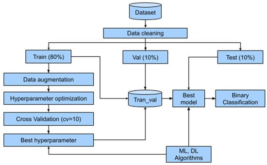
Figure 1.
Methodology used.
2.1. Materials
In the development of this research, the ULB dataset was used, which is available in [13]. The dataset comprises credit card transactions conducted by European cardholders in September 2013, capturing activity over a two-day period. In total, it contains 284,315 records for normal transactions and only 492 for the fraudulent class, representing a proportion of 0.173% of transactions out of the total records. This imbalanced dataset presents a significant challenge for analyzing and implementing ML and DL algorithms. This dataset consists of 31 descriptors, including the “class” label, which distinguishes normal transactions, represented by “0,” while fraudulent transactions are represented by “1”.
The different tests were conducted on a computer with an Intel (R) Core (TM) i7-8700T processor, 16GB RAM, running Windows 10 Pro X64 as the operating system. No GPU acceleration was used during model training or evaluation.
2.2. Data Processing
Data processing in ML is essential for obtaining more accurate predictions and more reliable results, which are crucial for making informed decisions. It allows for cleaning, transforming, and organizing information, thereby improving data quality [27]. An analysis of the dataset was conducted to identify features that had the same value across all records. The 30 available features were evaluated, and the results indicated that none of them met this condition, so no features were removed. This result is significant as it ensures that all features contribute variability to the model, which is essential for improving its generalization and accuracy.
Additionally, the dataset was checked for the presence of empty values, positive infinities, and negative infinities, and no records with these conditions were found. The absence of such values ensures the integrity of the dataset, preventing potential errors during the training process and enhancing the model’s stability. Subsequently, duplicate records were analyzed, identifying a total of 1081 duplicates, which were removed from the dataset. As a result of this process, the dataset was reduced to 283,726 records, of which 283,253 correspond to normal transactions and 473 to fraudulent transactions.
2.3. Synthetic Data Generation
The term synthetic data refers to data that are artificially created using computer simulations or algorithms rather than being collected from the real world [28]. In ML scenarios with highly imbalanced data, such as the dataset selected for this research, the minority class represents only 0.173% of the total records. This data imbalance can lead to biased models, compromising their ability to correctly classify the minority class. To address this challenge, new data were generated by adding Gaussian noise to the original minority class data. The noise is generated from a normal distribution, creating new synthetic points that simulate the inherent variability of the original data while remaining within the range of values for each descriptor in the dataset. Below is the mathematical description of the data augmentation method used.
- Data Preparation
The preprocessed dataset exhibits a relationship , explicitly represented as follows:
where each sample , is the value of each descriptor for the sample , and is the binary label. represents the set of normal transactions (majority class), while represents the set of fraudulent transactions (minority class).
Since , the number of samples in each subset is used to determine the number of synthetic samples for the minority class, denoted as , that need to be generated to balance the dataset. This is mathematically expressed as follows:
- Data Standardization
To perform data augmentation, the dataset of the minority class is standardized using the following expression:
where is the value of a feature in a sample , is the sample mean of , and is its standard deviation. This data transformation ensures that the features have a mean of 0 and a standard deviation of 1.
- Synthetic Data Generation
For iterations, a random r-dimensional value is added, defined as where and represent the standardized set of the minority class.
A perturbation is generated from the set of values , where the standard deviation is the parameter that controls the magnitude of the perturbation. This perturbation is then added to each .
A new synthetic point is created as follows:
It is important to restrict the values of the generated data so that they remain within the interval [0, 1]. For this reason, the following function is defined:
- Inverse Transformation
The newly generated sample is transformed back to the original space using the following expression:
The generated dataset is then added to the minority class , resulting in a balanced dataset.
2.3.1. Experimental Determination of the Value
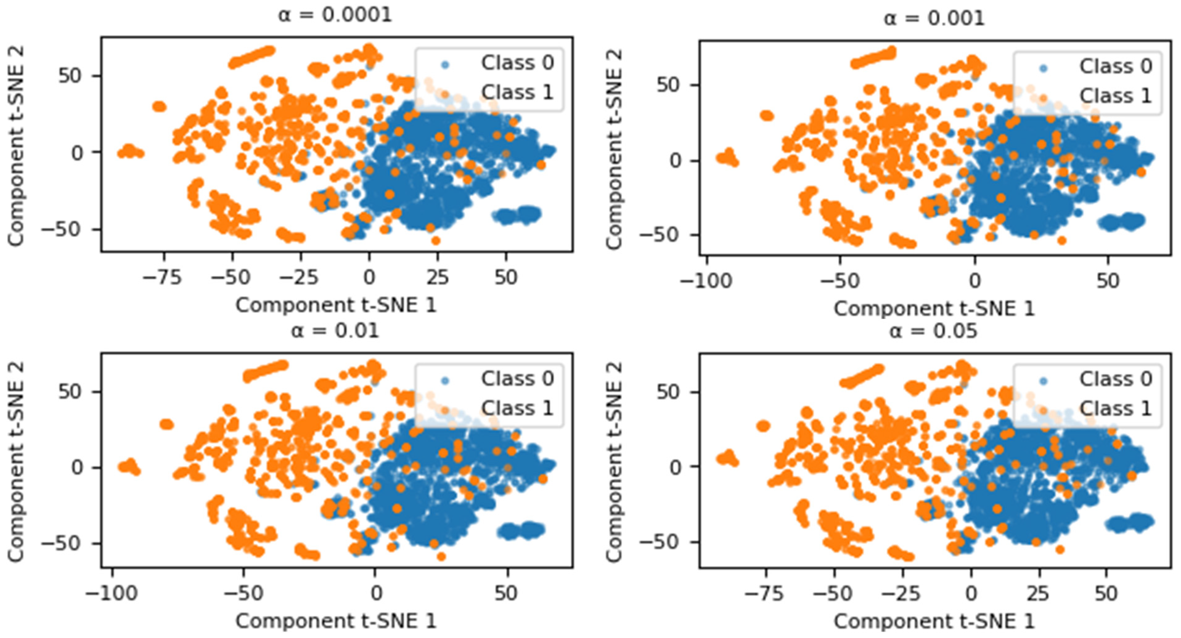
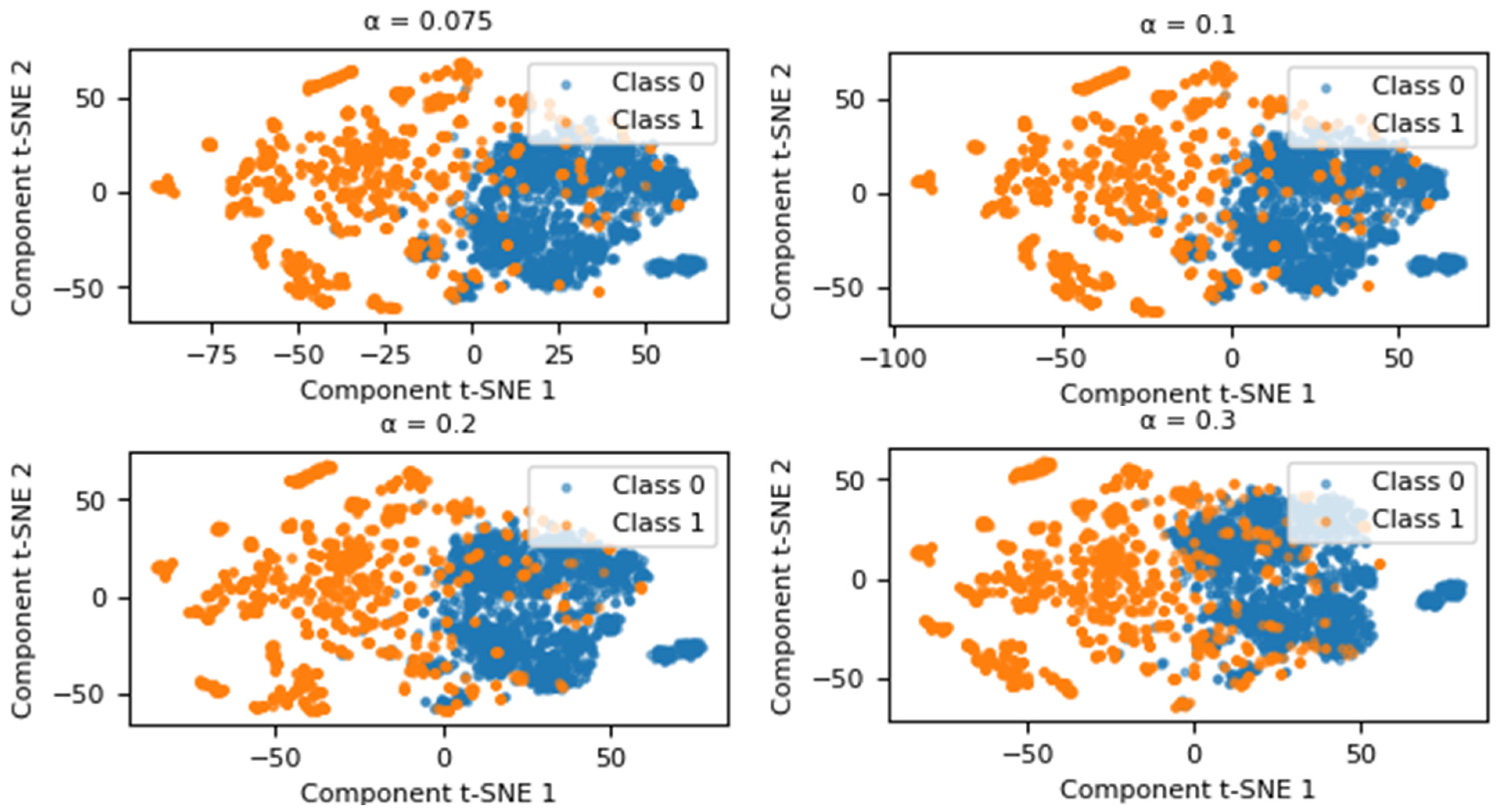
The generation of new data by adding Gaussian noise largely depends on the value of . To determine the best representativeness of the new data in relation to the original values, experiments were conducted with different values of . As shown in Figure 2, these experiments allowed the magnitude of the noise to be adjusted to achieve better data quality. T-SNE was used to visualize the data in two dimensions. The blue points represent the majority class (Class 0), while the orange points represent the minority class (Class 1).
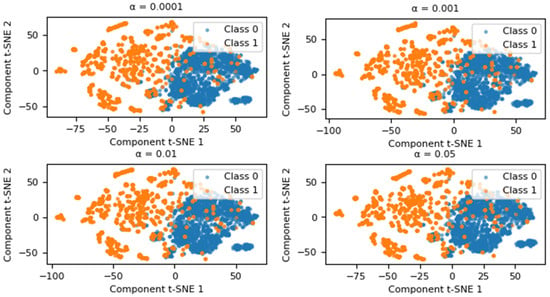

Figure 2.
Graphical representation using T-SNE for the value .
Based on this analysis, the impact of changing on the performance of a classifier has been evaluated. The XGBoost classifier was used as a reference, with its default hyperparameters set according to the Scikit-learn library. The classifier was evaluated using four metrics, the mathematical expressions of which are detailed in Section 2.6. The corresponding results are presented in Table 1. As the value of approaches 0, the classifier’s performance significantly improves across various evaluation metrics. Conversely, when is higher, the classifier’s performance is negatively affected by the presence of false positives and false negatives. Therefore, based on this analysis, it has been deemed appropriate to select . To validate the Gaussian nature of the generated data, statistical tests were conducted. The Shapiro–Wilk test yielded a statistic of 1.0030, while the Kolmogorov–Smirnov test produced a statistic of 0.0003. Both results confirm that the perturbations follow a Gaussian distribution, ensuring the synthetic data’s adherence to the desired statistical properties.

Table 1.
Performance of the XGBoost classifier for different alpha (α) values in the dataset.
2.3.2. Comparison of the Proposed Method with SMOTE and ADASYN
Considering the data augmentation method that introduces Gaussian noise, the dispersion of the generated data was analyzed in comparison with two oversampling techniques: SMOTE and ADASYN. Both techniques were implemented using the “imbalanced-learn” library, version 0.124, with default parameters.
As illustrated in Figure 3, the samples from both classes exhibit significant overlap, a trend that persists across different data augmentation methods. When examining the distribution of synthetic data generated with SMOTE, Class 1 shows an increase in quantity and dispersion; however, a noticeable overlap with Class 0 remains. This behavior is also evident in the synthetic dataset generated using ADASYN. In contrast, the dataset augmented with Gaussian noise demonstrates a clearer separation in less densely populated regions, improving representation compared to both the original dataset and the synthetic datasets generated by SMOTE and ADASYN.
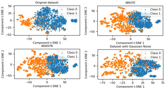
Figure 3.
Visualization of data distribution using oversampling techniques applied to the original dataset.
Gaussian noise, as a data augmentation technique, leverages its ability to introduce variability in the minority class without generating similar values, thereby mitigating the risk of overfitting associated with methods like SMOTE and ADASYN. Unlike these techniques, which create new instances by interpolating between real samples, Gaussian noise applies controlled perturbations based on a normal distribution, enhancing the diversity of the training set. This approach allows for the adjustment of noise magnitude through the standard deviation parameter (α), which is experimentally optimized as detailed in Section 2.3.1.
2.4. Classifiers
Classifiers were implemented using both machine learning (ML) techniques and a deep learning (DL) architecture to address the problem of bank fraud detection. The selection of ML classifiers, including XGBoost (XGB), Random Forest (RF), AdaBoost (ADA), and DecisionTree (DT), was based on multiple criteria such as interpretability, transparency, robustness to imbalanced data, and the ability to capture non-linear relationships between descriptors. Each of these classifiers was implemented using the Scikit-learn library.
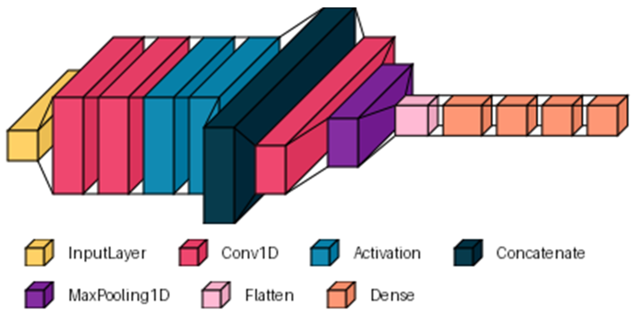
DL architecture in the context of fraud detection presents a promising solution [29,30]. In this study, a convolutional neural network (CNN) is presented, based on the model proposed in [31], to which a specific adaptation was made for the dataset used. Figure 4 presents the modified architecture, which consists of an input layer equal to the number of descriptors in the dataset. A parallel processing section is included, consisting of two convolutional branches. Each branch has 16 filters with different kernel sizes (7, 11). The outputs are merged using a concatenation layer that integrates the extracted features. Next, sequential processing is performed by adding a convolutional layer with 8 filters and a kernel size of 7, followed by a MaxPooling1D layer (pool_size = 2) to reduce data dimensionality. The output of this layer is flattened to feed into dense layers that learn more abstract representations of the data. Three dense classification layers with 256, 120, and 64 neurons were added to the architecture. The convolutional and dense layers used the ‘ReLU’ activation function. Finally, a dense layer with a single neuron and a ‘sigmoid’ activation function was added for binary classification.

Figure 4.
General structure of the DL architecture based on CNN.
2.5. Hyperparameter Optimization
Hyperparameter optimization (HPO) is the process of adjusting the values that control the behavior of an ML or DL model to improve its performance [32]. For this purpose, HyperOpt was chosen, a library based on the Tree of Parzen Estimators (TPE) algorithm, which makes it more efficient and faster than traditional methods like GridSearch [27], as it explores the hyperparameter space more intelligently, reducing computation time without compromising model quality. In the implementation, HyperOpt was configured using the Tree-structured Parzen Estimator (TPE) algorithm through the fmin function. A custom search space (dt_space) was defined, the tpe.suggest method was used for hyperparameter selection, and a maximum of 5 evaluations (max_evals = 5) was set. Additionally, trials objects were used to record the results of each iteration, enabling detailed tracking of the optimization process.
These hyperparameters, such as the depth of a decision tree or the learning rate for the different classifiers used, are defined in Table 2. To establish the range of values for these hyperparameters, a 1% sample of the training subset was selected, and the model was tuned using HyperOpt. This optimization process was evaluated using the accuracy metric. If the accuracy value was below 99%, the range of hyperparameter values was updated, exploring new values until the desired results were achieved.

Table 2.
Hyperparameter space used for the classifiers.
2.6. Performance Evaluation
In the performance evaluation, an experimental protocol was implemented that considered its application both on the original dataset and on the synthetic datasets generated using the selected sampling techniques and the proposed method. For the ML classifiers and DL architecture, the dataset partitioning was performed using a stratified random sampling scheme, assigning 80% of the instances to the training set, 10% to the validation set, and the remaining 10% to the test set.
The CNN was trained for 10 epochs, with a batch size of 64, using the Adam optimizer, a learning rate of 0.001, and the loss function “binary_crossentropy”, suitable for binary classification problems. During this phase, callbacks were included to improve the generalization ability of the models and avoid overfitting. The callbacks included ModelCheckpoint, which saves the model with the best score (monitor = ‘val_accuracy’) on the test set; ReduceLROnPlateau, with monitor = “val_loss”, factor = 0.1, patience = 3, and min_lr = 1 × 10⁻⁷. Additionally, CSVLogger was used to log the training progress to a CSV file, TensorBoard to visualize the training and validation metrics, and EarlyStopping to stop the training if “val_loss” did not improve after four epochs. These callbacks were used to enhance the performance and generalization of each model during this phase.
The performance evaluation of the ML classifiers and CNN was based on the use of multiple metrics widely validated in the literature, including accuracy, precision, sensitivity, F1-score, area under the curve (AUC), the Matthews correlation coefficient (MCC), geometric mean (G-Mean), and balanced accuracy index (IBA) [33,34,35]. These metrics allow for a comprehensive evaluation of the classifiers’ performance, considering various critical aspects such as the balance between true positives and negatives, discriminative ability, and robustness against class imbalance. Their mathematical expressions are described as follows:
where , , and represent the number of true positives, false positives, true negatives, and false negatives, respectively.
3. Results
In this section, the results obtained after evaluating the different ML classifiers and the CNN architecture on the original dataset and the synthetic datasets generated by SMOTE, ADSAYN, and the proposed method are presented.
The results of the best hyperparameters obtained for the different classifiers are summarized in Table 3, where RF, XGB, and CNN achieved the highest accuracy scores on the training and validation subsets, compared to the ADA and DT classifiers, which showed the lowest results. This indicates that, although they are useful models, their performance does not reach the level of the other classifiers in this context.

Table 3.
Best hyperparameters of the classifiers evaluated on the training and validation subset.
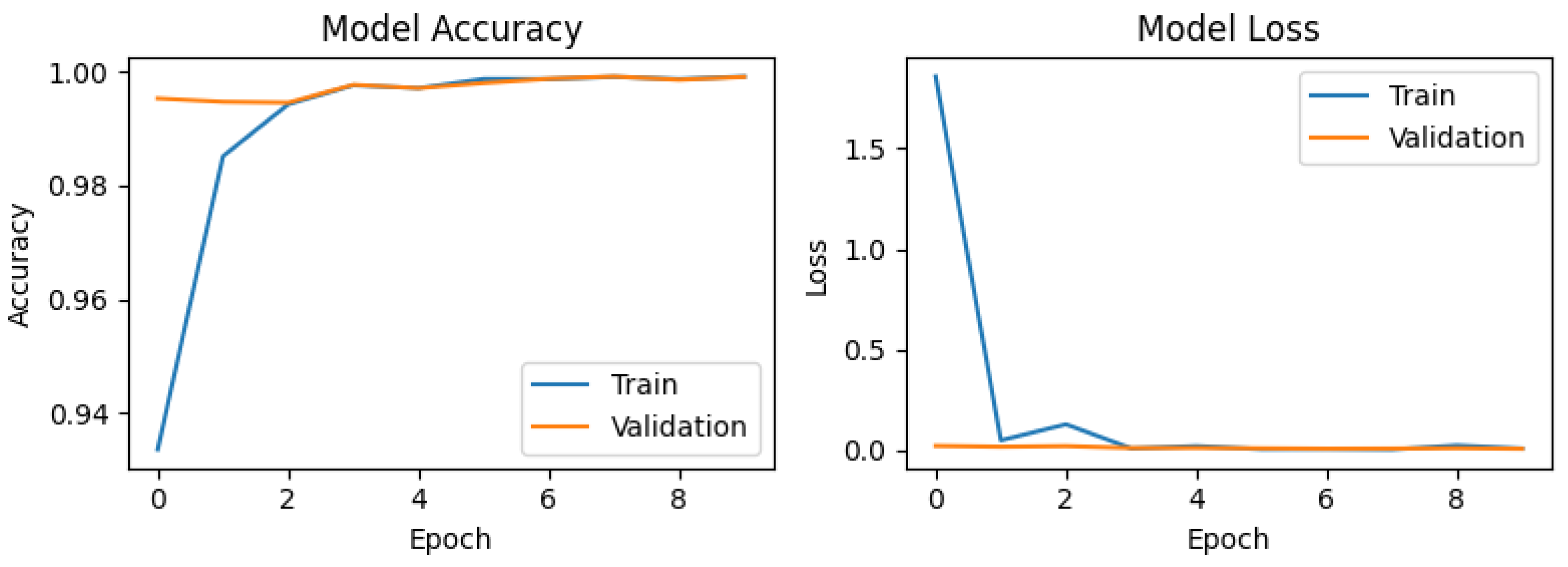
In Figure 5, Figure 6, Figure 7 and Figure 8, the training and validation behavior of the CNN is presented, which is a standard analysis in classification tasks. These results highlight two fundamental metrics: accuracy and loss. For the original dataset (Figure 5), the accuracy graph shows a rapid improvement during the first epoch for both the training curve (blue line) and the validation curve (orange line). This behavior is expected, as CNNs are capable of efficiently learning distinctive patterns. However, a slight drop in training accuracy is observed at epoch 4, likely due to minor fluctuations during the optimization process. The model quickly recovers in subsequent epochs, aided by the callback mechanism, achieving a maximum validation accuracy (val_accuracy) of 0.99961. The loss plot exhibits consistent behavior, with a sharp decline during the first epoch, starting from values near 3 and stabilizing close to 0. This indicates efficient convergence without signs of overfitting.

Figure 5.
Training and validation performance of the CNN on the original dataset.

Figure 6.
Training and validation performance of the CNN using synthetic data generated with SMOTE.
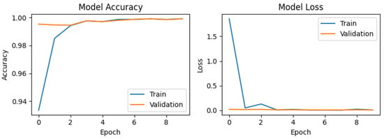
Figure 7.
Training and validation performance of the CNN using synthetic data generated with ADASYN.

Figure 8.
Training and validation performance of the CNN using synthetic data generated with the proposed method.
For the synthetic dataset generated using SMOTE (Figure 6), the accuracy graph exhibits stable behavior with significant improvement, achieving the highest validation accuracy (val_accuracy) score of 0.99937. This performance can be attributed to the increased diversity of the training set, which enhances the model’s generalization capability. The loss graph demonstrates a sharp decline during the first epoch, decreasing from values close to 2.5 to near 0, indicating rapid assimilation of the patterns present in the synthetic data. A similar trend is observed for the ADASYN generated dataset (Figure 7), which attains a val_accuracy of 0.99912. The loss graph for ADASYN also shows a pronounced initial decrease followed by stabilization, reflecting adequate model convergence. Finally, for the dataset augmented with Gaussian noise (Figure 8), the accuracy plot yields a val_accuracy of 0.99944. This result suggests that the introduction of Gaussian noise enhances model robustness by increasing variability in the training and validation data. Collectively, these results demonstrate the CNN’s high effectiveness in handling datasets with data augmentation techniques, maintaining stable performance and achieving near-perfect accuracy in all cases.
The values obtained for each of the confusion matrices were analyzed, revealing distinctive patterns in the performance of the classifiers across the different data augmentation methods for the test subset. Table 4, Table 5, Table 6 and Table 7 show the results of the confusion matrices for different classifiers applied to original and synthetic datasets generated with techniques such as SMOTE, ADASYN, and the proposed method. In general, it is observed that the CNN, XGB, and RF models tend to perform better in terms of TP and TN, with low FP and FN. ADA and DT show a higher number of FP, especially in the synthetic datasets, suggesting lower accuracy in classification. The synthetic data generated with SMOTE and the proposed method slightly improve performance compared to ADASYN, which shows a significant increase in FP.

Table 4.
Confusion matrix results for the original dataset.

Table 5.
Confusion matrix results for the synthetic dataset generated with SMOTE.

Table 6.
Confusion matrix results for the synthetic dataset generated with ADASYN.

Table 7.
Confusion matrix results for the synthetic dataset generated with the proposed method.
Based on the values of the confusion matrices described previously, a comparison of the performance of the classifiers applied to the different datasets was made. For the original dataset (Table 8), RF stands out as the most balanced model, excelling in multiple evaluation metrics: accuracy (0.999471), which quantifies the overall precision of the model; precision (1.0), which evaluates the proportion of correct positive predictions; F1-score (0.794521), which represents the harmonic mean between precision and recall; AUC (0.999471), which measures the discriminative ability of the model between classes; and MCC (0.811629), which provides a balanced measure even with imbalanced classes. However, the CNN outperformed Random Forest in three specific metrics: recall (0.681818), which quantifies the proportion of correctly identified positive cases; G-Mean (0.825679), which evaluates the balance between sensitivity and specificity; and IBA (0.464899), which adjusts precision considering class imbalance. These results suggest that, while Random Forest shows superior performance in most global metrics, the CNN demonstrates greater robustness in identifying positive cases and handling class imbalance. However, RF presents the highest training time of 803.3527 s, compared to the other classifiers.

Table 8.
Evaluation metrics, training time, and inference time for the original dataset.
For the data augmentation technique with SMOTE, outstanding performance is observed in most of the evaluated models (Table 9). The RF algorithm demonstrates exceptional performance in key metrics such as accuracy (0.999471), precision (0.939394), F1-score (0.805195), AUC (0.999471), and MCC (0.813300). XGB shows very similar performance, with slightly lower values, but stands out for its computational efficiency, with significantly lower training time (5.3062 s compared to RF’s 769.6016 s) and competitive inference time (0.0662 s). The CNN, while maintaining excellent performance with metrics such as accuracy (0.999295) and AUC (0.999295), requires the highest training time (483.0183 s) and inference time (2.5536 s). ADA and DT show more modest performance compared to the other classifiers. In general, RF and XGB stand out as the most balanced models in terms of accuracy and efficiency, while CNN, although precise, is less efficient in terms of computational time.

Table 9.
Evaluation metrics, training time, and inference time for the synthetic dataset generated with SMOTE.
For ADASYN (Table 10), it is observed that XGB stands out as the model with the best overall performance, achieving the highest accuracy (0.861111), F1-score (0.775000), AUC (0.999365), and MCC (0.778599), along with efficient training and inference times (4.7077 s and 0.0772 s, respectively). RF also shows solid performance, with metrics close to those of XGB, although with a significantly higher training time (1300.1717 s). The CNN, while having competitive accuracy (0.998696), shows lower precision (0.561404) and a longer inference time (2.6097 s). ADA and DT show more modest performance, with notably lower precision and F1-score, although ADA has a high recall (0.795455) and a superior G-mean (0.881926), indicating a better ability to balance the detection of positive and negative classes. Overall, XGB and RF stand out as the most balanced models in terms of accuracy and efficiency, while ADA and DT are less precise but useful in scenarios where recall is prioritized.

Table 10.
Evaluation metrics, training time, and inference time for the synthetic dataset generated with ADASYN.
Finally, for the proposed data augmentation method based on Gaussian noise (Table 11), it is observed that XGBoost stands out as the model with the best overall performance, achieving the highest accuracy (0.999507), precision (0.96875), F1-score (0.815789), AUC (0.999506), and MCC (0.825936), along with efficient training and inference times (5.0046 s and 0.0973 s, respectively). RF also shows solid performance, with metrics close to those of XGBoost, although with a higher training time (512.0690 s). The CNN maintains competitive accuracy (0.999401) and AUC (0.9994) but requires longer training and inference times (421.0122 s and 2.3840 s, respectively). ADA shows more modest performance, specifically in recall (0.772727), G-mean (0.867869), and IBA (0.601053), indicating a better ability to detect positive cases. Overall, XGB and RF stand out as the most balanced models in terms of accuracy and efficiency, while ADA and DT are less precise but useful in scenarios where recall is prioritized.

Table 11.
Evaluation metrics, training time, and inference time for the synthetic dataset generated with the proposed Gaussian noise method.
The results highlight the superiority of Gaussian noise-based data augmentation over SMOTE and ADASYN, significantly enhancing the performance of XGBoost, CNN, and Random Forest classifiers. By introducing controlled perturbations via a normal distribution, Gaussian noise avoids the artificial similarity and class overlap inherent in SMOTE and ADASYN, methods reliant on interpolating existing samples. This approach not only increases training data diversity but also reduces overfitting risks by preventing redundant synthetic patterns, thereby improving model generalizability. The adjustable noise magnitude controlled by the standard deviation parameter α enables optimization of data realism and variability. Consequently, Gaussian noise-augmented datasets achieve near-perfect accuracy and robustness across all classifiers, demonstrating their efficacy in balancing minority class representation while maintaining the natural data distribution, a critical advantage for imbalanced classification tasks.
While Mehdi et al. [36] demonstrated that Gaussian Noise Upsampling (GNUS) underperformed SMOTE and ADASYN in enhancing Random Forest and XGBoost classifiers, our study addresses a critical gap in their methodology: the optimization of Gaussian noise’s standard deviation (α) and its impact on synthetic data quality. By systematically testing α values (Section 2.3), we identified optimal noise magnitudes that mitigate the limitations cited in [36], such as over-perturbation or insufficient variability. This refinement, combined with classifier hyperparameter tuning, enabled Gaussian noise-augmented data to achieve competitive performance in fraud detection—a finding with direct implications for financial institutions.
Our results suggest that Gaussian noise augmentation, when calibrated via α, offers a scalable and computationally efficient alternative to SMOTE/ADASYN for real-world fraud detection systems. Unlike interpolation-based methods, which risk generating artificial patterns, Gaussian noise preserves the statistical integrity of transactional data while diversifying minority-class samples. Financial institutions could adopt this approach to reduce false positives in fraud alerts, minimize operational costs linked to manual reviews, and improve customer trust through more reliable detection. Furthermore, the tunability of α allows institutions to adapt noise levels to specific fraud patterns (e.g., low-frequency high-risk transactions), enhancing model agility in dynamic financial environments. By resolving the “performance gap” noted in [36], this work provides a framework for responsibly integrating synthetic data into fraud detection pipelines. Policymakers and auditors could leverage these insights to establish guidelines for synthetic data usage in financial ML systems, ensuring robustness without compromising data authenticity.
4. Conclusions
This study comprehensively addressed the challenge of bank fraud detection in imbalanced datasets by proposing a Gaussian noise-based augmentation method to balance minority-class representation. By contrasting this approach with SMOTE and ADASYN, we demonstrated that injecting controlled perturbations into the minority class significantly enhances model accuracy while mitigating overfitting risks inherent in interpolation-based techniques. A rigorous evaluation using metrics such as MCC, G-Mean, and IBA revealed that XGBoost and CNN classifiers trained on Gaussian noise-augmented data achieved superior performance (accuracy: 0.999507, AUC: 0.999506), outperforming SMOTE and ADASYN across all metrics, including precision, recall, and F1-score.
The Gaussian noise method constitutes a practical solution for financial institutions to optimize their fraud detection systems in real operational environments. Its implementation in transactional monitoring systems allows for significantly reducing false positives without compromising the detection of infrequent fraudulent patterns. The combination of its computational efficiency and compatibility with established ML classifiers (such as XGBoost) facilitates gradual adoption without requiring substantial modifications to existing infrastructure. A key differentiating aspect is the adjustable α parameter, which enables the adaptation of data augmentation levels to different fraud typologies, including high-value low-frequency transactions or new cyberattack vectors.
Unlike techniques such as SMOTE and ADASYN, which generate synthetic data through interpolation, the Gaussian noise-based approach maintains the original statistical distribution, considerably reducing the risk of overfitting. However, its effectiveness is subject to two fundamental conditions: the quality of the original data and precise calibration of the α parameter to avoid data distortions. These considerations are very important to achieve the ideal balance between data diversity and predictive accuracy in real banking applications.
As future research lines, we propose the following: the incorporation of real-time adaptive deep learning architectures (such as transformers) and multi-institutional datasets to improve model generalization; exploring the correlation between the proposed Gaussian noise-based synthetic data generation method and high-level cryptography techniques, such as chaotic systems which could add an additional layer of security and variability to the data, further improving the robustness of fraud detection models; and lastly, establishing collaborations with regulatory bodies to develop standards for the use of synthetic data, thereby accelerating its industrial adoption and ensuring more robust protection against fraud in the context of constantly evolving digital economies.
Author Contributions
Conceptualization, methodology, validation, data curation, and formal analysis, F.L.B.-S., H.A.-V., and M.G.F.; software, investigation, resources, writing—original draft preparation, project administration, funding acquisition, and visualization, F.L.B.-S.; writing—review and editing, F.L.B.-S. and M.G.F.; supervision, M.G.F. All authors have read and agreed to the published version of the manuscript.
Funding
This research received no external funding, and the APC was funded by Universidad Señor de Sipán (Peru).
Institutional Review Board Statement
Not applicable.
Informed Consent Statement
Not applicable.
Data Availability Statement
The data presented in this study are available on request from the corresponding author.
Conflicts of Interest
The authors declare no conflicts of interest.
References
- Hasan, M.; Hoque, A.; Le, T. Big Data-Driven Banking Operations: Opportunities, Challenges, and Data Security Perspectives. FinTech 2023, 2, 484–509. [Google Scholar] [CrossRef]
- Chaturvedi, K.; Goel, P.K.; Bansal, Y.K.; Kaushik, T.; Sharma, A.; Srivel, R. Fin Safe—Empowering Financial Security through the Synergy of Machine Learning and Blockchain. In Proceedings of the 2024 10th International Conference on Communication and Signal Processing (ICCSP), Melmaruvathur, India, 12–14 April 2024. [Google Scholar] [CrossRef]
- Hilal, W.; Gadsden, S.A.; Yawney, J. Financial Fraud: A Review of Anomaly Detection Techniques and Recent Advances. Expert. Syst. Appl. 2022, 193, 116429. [Google Scholar] [CrossRef]
- Shahana, T.; Lavanya, V.; Bhat, A.R. State of the art in financial statement fraud detection: A systematic review. Technol. Forecast. Soc. Chang. 2023, 192, 122527. [Google Scholar] [CrossRef]
- Alatawi, M.N. Detection of fraud in IoT based credit card collected dataset using machine learning. Mach. Learn. Appl. 2025, 19, 100603. [Google Scholar] [CrossRef]
- Banca por Internet. Es tiempo de ir por más—Interbank. Available online: https://interbank.pe/comunicado (accessed on 27 November 2024).
- Mashrur, A.; Luo, W.; Zaidi, N.A.; Robles-Kelly, A. Machine Learning for Financial Risk Management: A Survey. IEEE Access 2020, 8, 203203–203223. [Google Scholar] [CrossRef]
- Ruchay, A.; Feldman, E.; Cherbadzhi, D.; Sokolov, A. The Imbalanced Classification of Fraudulent Bank Transactions Using Machine Learning. Mathematics 2023, 11, 2862. [Google Scholar] [CrossRef]
- Eroglu, D.Y.; Pir, M.S. Hybrid Oversampling and Undersampling Method (HOUM) via Safe-Level SMOTE and Support Vector Machine. Appl. Sci. 2024, 14, 10438. [Google Scholar] [CrossRef]
- Le, T.P.; Rho, C.; Min, Y.; Lee, S.; Choi, D. A2GAN: A Deep Reinforcement-Based Learning Algorithm for Risk-Aware in Finance. IEEE Access 2021, 9, 137165–137175. [Google Scholar] [CrossRef]
- Aburbeian, A.M.; Fernández-Veiga, M. Secure Internet Financial Transactions: A Framework Integrating Multi-Factor Authentication and Machine Learning. AI 2024, 5, 177–194. [Google Scholar] [CrossRef]
- Credit Card Fraud Detection. Available online: https://www.kaggle.com/datasets/mlg-ulb/creditcardfraud (accessed on 28 November 2024).
- Le, T. Dataset for Evaluate A2GAN Paper. Available online: https://ieee-dataport.org/documents/dataset-evaluate-a2gan-paper (accessed on 28 November 2024).
- Lopez-Rojas, E.; Elmir, A.; Axelsson, S. PaySim: A Financial Mobile Money Simulator for Fraud Detection. Available online: https://urn.kb.se/resolve?urn=urn:nbn:se:bth-13651 (accessed on 28 November 2024).
- Aburbeian, A.M.; Ashqar, H.I. Credit Card Fraud Detection Using Enhanced Random Forest Classifier for Imbalanced Data. In Proceedings of the 2023 International Conference on Advances in Computing Research (ACR’23), Orlando, FL, USA, 8–10 May 2023; Daimi, K., Al Sadoon, A., Eds.; Springer Nature: Cham, Switzerland, 2023; pp. 605–616. [Google Scholar] [CrossRef]
- Wijaya, M.G.; Pinaringgi, M.F.; Zakiyyah, A.Y.; Meiliana. Comparative Analysis of Machine Learning Algorithms and Data Balancing Techniques for Credit Card Fraud Detection. Procedia Comput. Sci. 2024, 245, 677–688. [Google Scholar] [CrossRef]
- Huang, H.; Liu, B.; Xue, X.; Cao, J.; Chen, X. Imbalanced credit card fraud detection data: A solution based on hybrid neural network and clustering-based undersampling technique. Appl. Soft Comput. 2024, 154, 111368. [Google Scholar] [CrossRef]
- Ahsan, M.M.; Ali, M.S.; Siddique, Z. Enhancing and improving the performance of imbalanced class data using novel GBO and SSG: A comparative analysis. Neural Netw. 2024, 173, 106157. [Google Scholar] [CrossRef]
- Shi, F.; Zhao, C. Enhancing financial fraud detection with hierarchical graph attention networks: A study on integrating local and extensive structural information. Financ. Res. Lett. 2023, 58, 104458. [Google Scholar] [CrossRef]
- Mytnyk, B.; Tkachyk, O.; Shakhovska, N.; Fedushko, S.; Syerov, Y. Application of Artificial Intelligence for Fraudulent Banking Operations Recognition. Big Data Cogn. Comput. 2023, 7, 93. [Google Scholar] [CrossRef]
- Nobel, S.M.N.; Sultana, S.; Singha, S.P.; Chaki, S.; Mahi, M.J.N.; Jan, T.; Barros, A.; Whaiduzzaman, M. Unmasking Banking Fraud: Unleashing the Power of Machine Learning and Explainable AI (XAI) on Imbalanced Data. Information 2024, 15, 298. [Google Scholar] [CrossRef]
- Du, H.; Lv, L.; Guo, A.; Wang, H. AutoEncoder and LightGBM for Credit Card Fraud Detection Problems. Symmetry 2023, 15, 870. [Google Scholar] [CrossRef]
- Sulaiman, S.S.; Nadher, I.; Hameed, S.M. Credit card fraud detection using improved deep learning models. Comput. Mater. Contin. 2024, 78, 1049–1069. [Google Scholar] [CrossRef]
- Yousefimehr, B.; Ghatee, M. A distribution-preserving method for resampling combined with LightGBM-LSTM for sequence-wise fraud detection in credit card transactions. Expert Syst. Appl. 2025, 262, 125661. [Google Scholar] [CrossRef]
- Lu, S.; Ye, J. Imbalanced data classification scheme based on G-SMOTE. Procedia Comput. Sci. 2024, 247, 1295–1303. [Google Scholar] [CrossRef]
- Lv, H.; Du, Y.; Zhou, X.; Ni, W.; Ma, X. A Data Enhancement Algorithm for DDoS Attacks Using IoT. Sensors 2023, 23, 7496. [Google Scholar] [CrossRef]
- Becerra-Suarez, F.L.; Fernández-Roman, I.; Forero, M.G. Improvement of Distributed Denial of Service Attack Detection through Machine Learning and Data Processing. Mathematics 2024, 12, 1294. [Google Scholar] [CrossRef]
- ¿Qué son los datos sintéticos? Available online: https://www.ibm.com/es-es/topics/synthetic-data (accessed on 29 November 2024).
- Mienye, I.D.; Swart, T.G. A Hybrid Deep Learning Approach with Generative Adversarial Network for Credit Card Fraud Detection. Technologies 2024, 12, 186. [Google Scholar] [CrossRef]
- Tayebi, M.; El Kafhali, S. Generative Modeling for Imbalanced Credit Card Fraud Transaction Detection. J. Cybersecur. Priv. 2025, 5, 9. [Google Scholar] [CrossRef]
- Becerra-Suarez, F.L.; Tuesta-Monteza, V.A.; Mejia-Cabrera, H.I.; Arcila-Diaz, J. Performance Evaluation of Deep Learning Models for Classifying Cybersecurity Attacks in IoT Networks. Informatics 2024, 11, 32. [Google Scholar] [CrossRef]
- Raiaan, M.A.K.; Sakib, S.; Fahad, N.M.; Mamun, A.A.; Rahman, M.A.; Shatabda, S.; Mukta, M.S.H. A systematic review of hyperparameter optimization techniques in Convolutional Neural Networks. Decis. Anal. J. 2024, 11, 100470. [Google Scholar] [CrossRef]
- Zhu, Q. On the performance of Matthews correlation coefficient (MCC) for imbalanced dataset. Pattern Recognit. Lett. 2020, 136, 71–80. [Google Scholar] [CrossRef]
- García, V.; Mollineda, R.A.; Sánchez, J.S. Index of Balanced Accuracy: A Performance Measure for Skewed Class Distributions. In Pattern Recognition and Image Analysis; Springer: Berlin/Heidelberg, Germany, 2009; pp. 441–448. [Google Scholar] [CrossRef]
- Chicco, D.; Warrens, M.J.; Jurman, G. The Matthews Correlation Coefficient (MCC) is More Informative Than Cohen’s Kappa and Brier Score in Binary Classification Assessment. IEEE Access 2021, 9, 78368–78381. [Google Scholar] [CrossRef]
- Imani, M.; Beikmohammadi, A.; Arabnia, H.R. Comprehensive Analysis of Random Forest and XGBoost Performance with SMOTE, ADASYN, and GNUS Under Varying Imbalance Levels. Technologies 2025, 13, 88. [Google Scholar] [CrossRef]
Disclaimer/Publisher’s Note: The statements, opinions and data contained in all publications are solely those of the individual author(s) and contributor(s) and not of MDPI and/or the editor(s). MDPI and/or the editor(s) disclaim responsibility for any injury to people or property resulting from any ideas, methods, instructions or products referred to in the content. |
© 2025 by the authors. Licensee MDPI, Basel, Switzerland. This article is an open access article distributed under the terms and conditions of the Creative Commons Attribution (CC BY) license (https://creativecommons.org/licenses/by/4.0/).


