Traffic Similarity Observation Using a Genetic Algorithm and Clustering

Abstract

This article presents a technique of traffic similarity observation based on the statistical method of survival analysis by using a genetic algorithm. The basis comes from the k-means clustering algorithm. The observed traffic is collected from different network sources by using a NetFlow collector. The purpose of this technique is to propose a process of finding spread malicious traffic, e.g., ransomware, and considers the possibility of implementing a genetic-based algorithm. In our solution, a chromosome is created from clustering k-means centers, and the Davies–Bouldin validity index is used as the second fitness value in the solution.

1. Introduction

Recently, the computer world has been facing problems with many types of cyber-attacks. Attackers use malicious software or codes to obtain the privileged rights to clients’ computers. Ransomware [1] is one such malicious code. Typically, it generates cyclically repetitive communication with command and control points or nonexistent domains. This behavior can produce an anomaly that can be observed and analyzed.

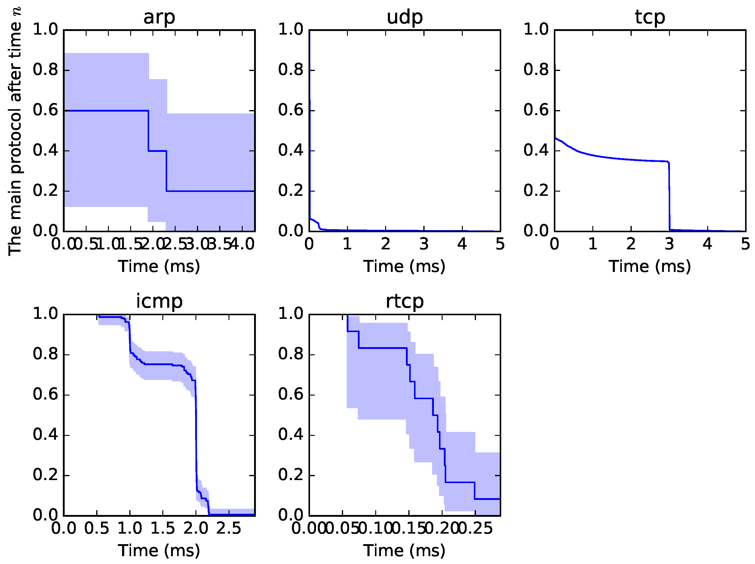
Based on previous research [2], we found a possible way to filter traffic and collect such repetitive behavior. We used survival analysis [3] and NetFlow messages [4] collected from Cisco network devices. The analysis creates survival curves [5] of origin–destination traffic in a specific time window. A sample of the graphical output from the survival analysis can be seen in Figure 1. All traffic can be examined from such a perspective, not to observe the proper survival time but to determine a format or pattern of traffic. Each curve is unique, as it depends on the type of traffic. The blue part is called “confidence intervals” and is the measure of possible variability.

We have implemented our genetic cluster algorithm to find the similarity or closeness of each curve as part of the continuous development of our genetic decision probe (GDP) application [6]. An output of our analysis is the clustering of traffic into groups based on the minimum Euclidean distance. In principle, if there is network traffic displayed in the presented curves, it is possible to compare the similarity of such curves. This can be done by the presented algorithm. This may be useful, for example, for detecting the repetitive traffic of ransomware from captured data in different parts of the network that would otherwise look like normal network traffic.

This article presents the idea and compares our genetic-based algorithm with a k-means algorithm, which was also programmed by our team. The idea is to use a genetic algorithm instead of the common approach to develop an auto-adaptive and extendible solution for an field-programmable gate array (FPGA) [7] hardware system, and we compare each of the proposed and considered algorithms with the classical one.

2. Related Work

Genetic algorithms are often used to improve current detection methods. We can find many articles related to this topic and why genetic algorithms are a useful solution. In [8], the authors used a genetic algorithm to extract data in principal component analysis (PCA). In [9], the authors applied it to the calculation of matrices of Euclidean distance. Related to the clustering problem and the use of genetic algorithms (GAs), in the past, many applications based on genetic clustering algorithms were developed. They use different representations for chromosomes, fitness functions, crossover, etc.

In [10], they presented a solution that uses a genetic algorithm with gene rearrangement for K-means clustering. Here, each chromosome is described by a sequence of $M=N\ast K$ real-valued numbers, where N is the dimension of the feature space, and K is the number of clusters. For crossover, the path-based crossover operator has been used to build a path between two parent chromosomes.

In [11], the authors presented an efficient genetic algorithm-based clustering technique that utilizes the principles of a k-means algorithm. The chromosome is created in the same way. It is represented by a sequence of $N\ast K$ floating point numbers.

In their subsequent publication [12], the authors presented a genetic algorithm-based clustering technique, called GA-clustering. Generally, we can say that a chromosome is commonly created in two ways. The first solution maintains all centroids and data, and the second solution creates chromosomes only from centroids.

As a fitness measurement of an individual, the error measure from the minimum of the Euclidean distance is used, or a second measurement is added, for example, using a silhouette function. This second measureis used to measure the proportionality of centroids.

In our solution, a chromosome is created only from centroids, and the data are associated in each fitness observation. As the second measurement of the fitness, we used the Davies–Bouldin validity index.

Regarding FPGA and the possibility of implementing a genetic algorithm, for a full overview for readers, a genetic IP-based core was developed and tested in [13].

3. Algorithms

In this section, k-means and genetic-based algorithms are presented. First, the principle of using survival analysis is presented.

Survival Analysis

The survival function $S(t)$ is defined by Equation (1). This function defines the probability that, at the end of the event or equivalent, the probability of survival until at least t does not occur at time t [3].

$$S(t)=Pr(T>t)$$

(1)

where $0\le S(t)\le 1$, $F_T=1-S(t)$, and $F_T$ is the cumulative distribution function T, which means that $S(t)$ is a non-increasing function of t.

To estimate the survival function, a Kaplan–Meier analysis (2) or Cox estimate is used.

$$\widehat{S}(t)=\prod _{j=1}^k\left(\frac{n_j-d_j}{n_j}\right)=\widehat{S}(t)\left(1-\frac{d_t}{n_t}\right)$$

(2)

where $d_j$ corresponds to the number of events, eventually the number of completed events in time j. So far, $n_j$ is related to the number of objects that are still observed in time j. In our case of NetFLow traffic collection, we use this survival analysis function to create a gene expression matrix during a time window. The gene expression matrix is given as $GE{M}_{m,n}=m\times n$ for a time window $w(t)$, where m represents a set of solutions with n values; $m=\{n1,n2,\dots ,n(t)\}$ of the set m in a given linear space. The example of the $GE{M}_{m,n}$ for our genetic cluster algorithm is presented in

Table 1. Gene expression matrix.

IP Address	Survival function $\mathit{S}\mathbf{(}\mathit{t}\mathbf{)}$
192.168.1.66	1.00 0.73 0.64 0.45 0.45 0.27 0.18 0.18
192.168.1.255	1.00 0.42 0.42 0.28 0.14 0.14 0.07 0.00
89.176.9.204	1.00 1.00 0.66 0.32 0.00 0.00 0.00 0.00

.

We work further with these values. In this example, the first four values are the time line, and the other four values are the probabilities for the time-line values. The sizes of the time-line axis and the probability axis are not limited.

4. K-Means Algorithm

The k-means algorithm uses the Euclidean distance [14]. By taking two vectors $\overrightarrow{x}=(x_1,x_2,\dots ,x_n)$ and $\overrightarrow{y}=(y_1,y_2,\dots ,y_n)$ as a two-dimensional finding of values, the Euclidean distance between $\overrightarrow{x}$ and $\overrightarrow{y}$ is then defined by Equation (3):

$$d(\overrightarrow{x},\overrightarrow{y})=\sqrt{{(\overrightarrow{x}-\overrightarrow{y})}^{\prime }(\overrightarrow{x}-\overrightarrow{y})}.$$

(3)

Since each value contributes to the calculation of the Euclidean distance, the results can vary considerably, even with only a small change in the values. Generally, the k-means expression is defined as Equation (4):

$$\sum _{i=0}^n\underset{c_j\in C}{min}({\parallel x_j-c_i\parallel }^2)$$

(4)

where $c_j$ represents centroids, and C represents clusters. The k-means algorithm, which has been implemented in this study, is created using the Lloyd algorithm. The means $x\in X$ are the key values and are equal to ${min}_{c\in {\mathrm{I}\mathrm{R}}^d}{\sum }_{x\in X}{\parallel c-x\parallel }^2$. However, a simpler option is to use the distances $\overrightarrow{d}(x,c)={\parallel x-c\parallel }_2$. The slowest process, but one that reduces the restrictions previously described, is to choose the centroid $c_i$ according to $\{x\in X|{\varphi }_C(x)=c_i\}$. 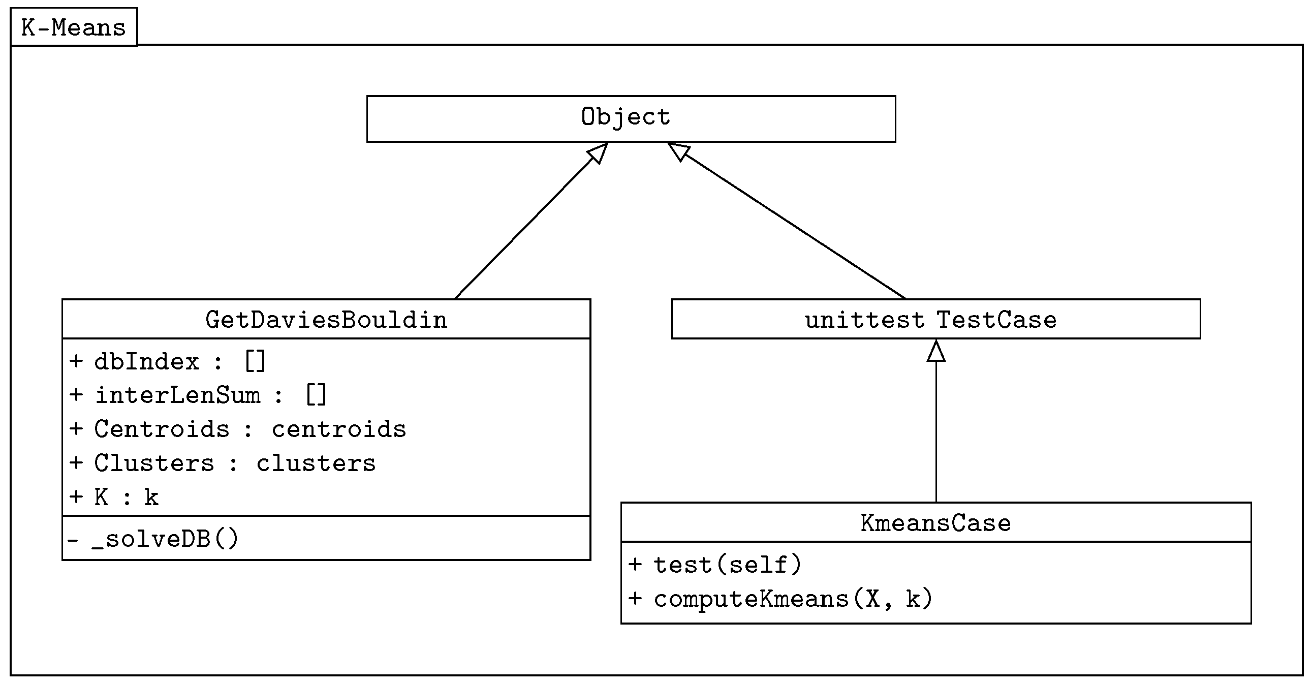The class diagram of our k-means algorithm is shown in Figure 2.

The class GetDaviesBouldin is used in both the k-means and genetic-based algorithms to verify the correct distribution of centroids. It is a separated imported class. It also returns the sum of the Euclidean distance values. The Davies–Bouldin validity index expression has the following equation, adopted from [15]:

$$\begin{array}{c}\hfill DB={\displaystyle \frac{1}{n}}\sum _{i=1}^n\underset{i\ne j}{max}\left\{{\displaystyle \frac{C_n(Q_i)+C_n(Q_j)}{C_n(Q_i,Q_j)}}\right\}\end{array}$$

(5)

where $C_n(Q_i)$ is the average distance inside the cluster from its center, and $C_n(Q_i,Q_j)$ is the distance between the clusters represented by centroids. The unittest TestCase [16] comes from the Python test package, and it is used here as the testing class. The main methods are implemented in the KmeansCase class, which takes the unittest as the object.

In the first step of the algorithm, $c_i=x_i\in X$ is chosen, and the Euclidian distance calculation of a member $x_i$ against centroid $c_i$ follows. This member is then inserted into the fittest group. The centroids are recomputed and replaced by the mean value of all members of a cluster $C_k$. The process is repeated until all members are assigned, as shown in Expression (6).

$$\begin{array}{c}\hfill C_k=\{x_n:\parallel x_n-c_k\parallel \le \forall \parallel x_n-c_k\parallel \}\\ \hfill c_k={\displaystyle \frac{1}{C_k}}\sum _{x_n\in C_k}{x}_n\end{array}.$$

(6)

In the next convergence step, the algorithm compares each member with its own cluster and the neighboring cluster from the Euclidean distance point of view. If a more appropriate cluster is selected, the member is moved to this cluster. This step is repeated until there are no more member shifts.

5. Genetic Algorithm

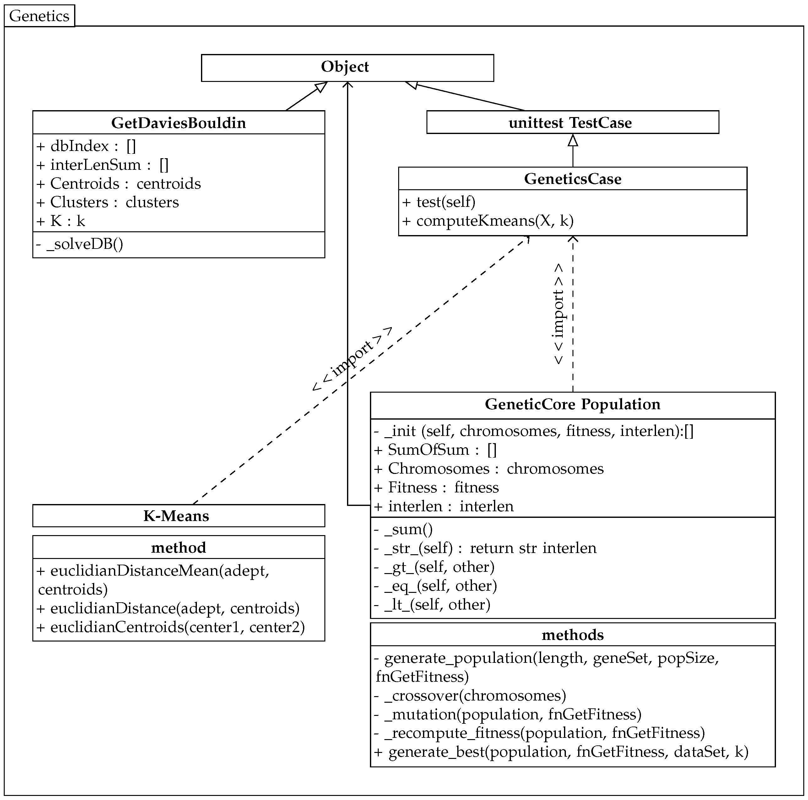
The implemented genetic algorithm uses the previously created k-means algorithm class, and its partial diagram is shown in Figure 3.

The genetic algorithm works with chromosomes that represent a solution to the problem. In this case, a chromosome represents k genes for k centroids $c_i$ of clusters C.

The chromosome or individual $\alpha$ and, consequently, the population P are determined in the first step according to Equation (7). A centroid $c_i=x_i$, and $x_i$ represents a vector of values ${\overrightarrow{x}}_i=\{n_1,n_2,\cdots ,n_M\}$, where n represents elements of the set M from the gene matrices.

$$\begin{array}{c}\hfill {\alpha }_i=({\overrightarrow{c}}_1,{\overrightarrow{c}}_2,\cdots ,{\overrightarrow{c}}_k)\in C|{\overrightarrow{c}}_k={\overrightarrow{c}}_i\in X\\ \hfill P=\{{\alpha }_1,{\alpha }_2,\cdots ,{\alpha }_C\}\end{array}.$$

(7)

The chromosome only keeps clusters’ centroids, and ${\overrightarrow{x}}_i$ values are associated with this centroid just when evaluating an individual’s fitness. The ${\overrightarrow{x}}_i$ valuesare released after the fitness evaluation.

The Euclidean distance and the Davies–Bouldin validity index are used to evaluate an individual. The genetic algorithm minimizes the sum of the Euclidean distance for all individual clusters. Expression (8) is the objective function $f(\alpha )$ of the problem.

$$\begin{array}{c}\hfill \mathrm{minimize}\sum _{k=1}^K\sum _{x_n\in C_k}{\parallel {\mathbf{x}}_n-{\overrightarrow{c}}_k\parallel }^2\\ \hfill \mathrm{according}\mathrm{to}{\overrightarrow{c}}_k,C_k\end{array}.$$

(8)

The criteria, i.e., the individual’s (chromosome) evaluation, are based on the sum of the mean distances inside the clusters, i.e., $f(\alpha )\wedge fi{t}_1(\alpha )$ and $\forall {\alpha }_i\in P:0<f{(\alpha )}_1<f{(\alpha )}_2$. For example, for the number of clusters $C=4$, $k=4$, the individual contains four genes, with each gene representing the solution of one cluster. An example of the output is presented in

Table 2. The sum of the mean distances inside the clusters.

Mean Distances Inside Clusters				Sum
0.0	0.0	0.0	1.5871699711831	1.5871699711831

.

The genetic algorithm selects individuals with the lowest value of the sum of the average distances in the population P. To simplify the running of the algorithm, this method is called from the imported custom class GetDaviesBouldin from the previous k-means solution. This class provides the calculation for the Davies–Bouldin validity index and returns its value to the dbIndex variable. This validity index is the second fitness measure.

The class population maintains the current population values, self.Chromosomes, and the evaluation of individuals in self.Fitness and self.interlen. This algorithm contains its own methods for comparing populations: OBJECT.__lt__(self, other) and eq, gt. Therefore, the minimum intra-cluster distance is always searched within two populations. One population represents the original population, and the other population is the same population after the crossover and mutation with the recalculated values of the fitness functions.

Thus, the evaluation of all populations is carried out in the framework of elitism. This is because the crossing is both vertical and horizontal between individuals in populations. Erroneous results (inf,null), broken down by zero, are filtered using the Python np.ma.masked_invalid package. This ensures that the wrong individuals are not selected. The crossover, mutation, and recalculation of fitness values are performed in each cycle. After that, populations are compared, and individuals are returned to those populations that satisfy the condition of choosing the best solution.

In the proposed solution, a method of crossing is created based on random selection, both in the chromosomes’ own genes and among the chromosomes. In the first step, the selected parts are crossed between the chromosomes, and the positions of the genes in the chromosomes are then changed. In this way, limiting the trapping of the solution in a local minimum is ensured.

Muting the solution ensures that there is no trapping at the local and global minima. In addition, this ensures that the current centroid values are not accidentally replaced by this mutation.

So far, centroid ${\overrightarrow{c}}_i$ is equal to ${\overrightarrow{x}}_i$. In this part of the performed mutation, the GetDaviesBouldin class returns the value of ${\overrightarrow{x}}_i\in C(k)$. The chromosome is then formed according to the following equation:

$$\begin{array}{c}\hfill {\alpha }_{i:\mathrm{new}}=({\overrightarrow{c}}_1,{\overrightarrow{c}}_2,\cdots ,{\overrightarrow{c}}_k)\in C|{\overrightarrow{c}}_k=⌀C(k)\\ \hfill P=\{{\alpha }_1,{\alpha }_2,\cdots ,{\alpha }_S\}\\ \hfill {\mathbf{c}}_{k:\mathrm{new}}={\overrightarrow{c}}_k={\overrightarrow{x}}_i|i,k:\Omega ⟶(1,N)\end{array}.$$

(9)

For example, a population with four chromosomes, each with three genes (three clusters), is created in the following format. An output from the GDP application is represented in

Table 3. Outputs of chromosomes from the genetic decision probe (GDP) application.

Chromosomes	Outputs	Chromosomes	Outputs
Chromosome 1	0.0 1.0 1000.0 0.0 0.79	Chromosome 3	0.0 1.0 1500.0 0.0 0.50
	0.0 1.0 1000.0 0.0 0.45		0.0 1.0 1500.0 0.0 0.37
	0.0 1.0 1000.0 0.0 0.45		0.0 1.0 1000.0 0.0 0.45
Chromosome 2	0.0 1.0 1500.0 0.0 0.37	Chromosome 4	0.0 1.0 0.0 0.0 0.00
	0.0 1.0 1000.0 0.0 0.45		0.0 1.0 0.0 0.0 0.00
	0.0 1.0 1500.0 0.0 0.37		0.0 1.0 1000.0 0.0 0.45

.

In this example, each chromosome expresses a vector of survival analysis values. The ranges of the chromosomes and the population can be extended.

6. Results of the Genetic Algorithm Implementation

In testing the framework of our solution, comparative tests of the k-means algorithm and the genetic algorithm for the driver and circle test kits were performed. The dataset of circles was imported from the Python package sklearn.datasets.samples_generator [17] and the dataset of drivers from [18].

The dataset of drivers includes 4000 records, and it is used to test the robustness of algorithms. The second dataset is used to test the convergence of algorithms. The individual outputs in

Table 4. The results of performed tests for both algorithms.

	Algorithms
Datasets	K-Means	GA	Tests
Drivers	8 cycles to convergence (4m, 16s) DB Index 0.5167630551103491 Sum: 29.107135396708152	6 cycles, population = 4 (1m, 2s) DB Index 0.46742701779860801 Sum: 27.452260723272207	Test 1
	5 cycles to convergence (1m, 59s) DB Index 0.6928435886081372 Sum: 38.22747907985817	2 cycles, population = 4 (23s) DB Index 0.67284260223514103 Sum: 29.601280430142346	Test 2
Cyrcles	6 cycles to convergence (3s, 926ms) DB Index 0.9987036150188133 Sum: 1.717726567997643	2 cycles, population = 4 (2s, 72ms) DB Index 0.77739787348584977 Sum: 1.5172548869635047	Test 1
	2 cycles to convergence (1s, 663ms) DB Index 0.9133526077302941 Sum: 1.6639746612808648	2 cycles, population = 6 (4s, 49ms) DB Index 0.97353773307594249 Sum: 1.7154716157662906	Test 2
	3 cycles to convergence (2s, 2ms) DB Index 0.8400359621183359 Sum: 1.4401091736722333	2 cycles, population = 10 (6s, 2ms) DB Index 0.8418532846822262 Sum: 1.5331916473395522	Test 3

and

Table 5. The results of performed tests for the genetic algorithm (GA) with manipulations.

Genetic Algorithm
Circles
2 cycles, population = 6 (4s, 49ms) DB Index 0.97353773307594249 Sum: 1.7154716157662906	Test 1 Cycles 2 Population 6	2 cycles, population = 10 (6s, 2ms) DB Index 0.8418532846822262 Sum: 1.5331916473395522	Test 3 Cycles 2 Population 10
6 cycles, population = 6 (9s, 738ms) DB Index 0.84332527741694963 Sum: 1.2663053983838712	Test 2 Cycles 6 Population 6	6 cycles, population = 10 (16s, 304ms) DB Index 0.89134036655984594 Sum: 1.4076740115353803	Test 4 Cycles 6 Population 10

show the observed values, which were the Davies–Bouldin validity indices and the average Euclidean distance in the data cluster. Furthermore, the time needed to run the algorithms was also monitored.

No dynamic increase or decrease in the number of centroids was expected with this solution. The results of the two algorithms were compared. Each test was run 10 times, and the best results are shown in the format of the GDP program console output. The distance number does not express a particular unit; it depends on what is being measured. The value “sum” represents the sum of the average distances in clusters. The lower score of the Davies–Bouldin index is better. Based on the repetition of the tests and the results, it can be concluded that GA had both faster data processing and a faster total calculation time. While increasing the population, the overall calculation time was increased. The processing time was also affected by data being read from datasets and by the hardware used.

7. Real Dataset of Traffic

The real dataset was imported during the application run from the GDP database into the supervisor module using the pandas:DataFrame package. An example of the composition of the custom dataset in an instance of the DataFrame is shown in

Table 6. Program output of the custom dataset.

N	IP Address	Survival Analysis Timeline					Timeline Values
0	89.176.9.204	0	1	1033	1041	1049	0	0.45	0.78	1.28	2.28
1	192.168.1.54	0	1	1501	1509	1553	0	0.37	0.44	0.51	0.58
2	79.143.185.229	0	1	0	0	0	0	0.00	0.00	0.00	0.00
3	192.168.1.46	0	1	1497	1501	1509	0	0.50	0.75	1.09	1.59
4	192.168.1.66	0	1	1033	1041	1049	0	0.79	0.88	0.98	1.09
N + 1

.

This dataset is a gene matrix for every source to destination (SD). This simple example verifies the possibilities of working with the output values of survival analysis and the resolution of individual survival curves. For explanation, the dataset represents a group of addresses that communicated through a peer-to-peer (P2P) network that excludes one IP address.

Using the genetic algorithm, individual clusters were assembled. These clusters represent the survival curves that are closest to the Euclidean distance with respect to its lowest centroid value. Again, the results of both algorithms, GA and k-means, were compared.

From this point of view, the k-means algorithm assigned similar courses to the same cluster. In the next step, the genetic algorithm was verified. The resulting output is the average distance within the cluster for each cycle. The k-means and GA results are shown in

Table 7. Program outputs of the final computation.

	Algorithms
Dataset	K-Means	GA	Tests
IP address	2 cycles to convergence, (78ms) DB Index 0.0016132173486533587 Sum: 0.9918338445433054   Near curve value, cluster 0: 79.143.185.229 Near curve value, cluster 1: 192.168.1.66 89.176.9.204 Near curve value, cluster 2: 192.168.1.54 192.168.1.46	GA, 4 cycles, population = 4 (142ms) Distance 1. cycle: [155.33340769869454] Distance 2. cycle: [4.218783667088422] Distance 3. cycle: [2.211733592974675] Distance 4. cycle: [0.9918338445433054] DB Index 0.0016132173486533587 Sum: 0.99183384454330537 Near curve value, cluster 0: 79.143.185.229 Near curve value, cluster 1: 89.176.9.204 192.168.1.66 Near curve value, cluster 2: 192.168.1.54 192.168.1.46	Test 1

. The GA minimization process of values can be seen in the same table. According to the similarity of curves and our awareness of where the IPs belong to, individual IP addresses were correctly assigned to clusters. These were IP addresses that communicated with each other.

8. Results

The genetic algorithm in the drivers–circles tests produced better results in terms of both the Davies–Bouldin validity index and the distribution of individuals in clusters depending on their Euclidean distance. In the case of the genetic algorithm, the result was no longer improved by increasing the number of iterations and the population sizes. The results are influenced by the initial random selection of centroids, as seen, for example, in the k-means algorithm in the driver dataset. Thus, the number of iterations and duration are both affected by this initial selection.

From a time perspective, the real-life example using the genetic algorithm was more demanding. Because of the algorithm profiling, it is time-consuming to create new instances of population classes. During repeated attempts, the error rate of the algorithm was determined, namely, the assignment of the same IP address to two different clusters. This error occurred when the algorithm ended the calculation with the output value of DB $\mathrm{value}>0.01$. Since the proposed GA algorithm works only with centroids as individuals and does not hold clustered data, as in the case of K-means, when a population is created using the random.choice method, a paradox of choosing the same centroid occurs with a small number of chromosomes. The genetic algorithm was then not able to correct the errors. This paradox can be influenced by increasing the number of chromosomes in the population, possibly increasing the value of the mutation.

The error has not occurred with more than 10 chromosomes in the population. If we compare the results of both algorithms, with a small number of input values, both algorithms reached the same degree of convergence. If the results with a large number of input values are compared, GA reaches a better time of convergence, taking into account the population size and the number of repetitions that have been fixed. In the case of a P2P real test, both algorithms correctly assigned the communicating IP addresses to clusters. This was a traffic connection negotiation.

9. Conclusions

In this article, we presented the comparison and testing of k-means and genetic algorithms. These algorithms were used to search for the similarity of survival curves. The idea behind this is that a certain type of network traffic can be observed by converting it to specific traffic curves using a survival analysis method and then comparing the individual curves. Comparing curves of different network nodes—for example, in peer-to-peer repetitive behavior or ransomware generating requests in certain periodic cycles—might be useful in finding unwanted traffic.

Therefore, we decided to test algorithms capable of performing the above calculation. We were able to improve our genetic algorithm and decrease the time needed to find the solution by not calling new classes of populations through crossover and mutation. The results show that the genetic algorithm is better suited for the calculation of a larger number of survival curves. Algorithm efficiency and the tuning of individual settings, such as the population size or number of iterations, must be taken into account. Both algorithms correctly assigned the IP addresses in the test set relative to their generated traffic.

Our continuing work is focused on automatically increasing or decreasing the number of centroids to make the algorithm more effective and on parallelization. The source code is available on request.