Applying Machine Learning to DEM Raster Images

Abstract

Geospatial data analysis can be improved by using data-driven algorithms and techniques from the machine learning field. The aim of our research is to discover interrelationships among topographical data to support the decision-making process. In this paper, we extracted topographical geospatial data from digital elevation model (DEM) raster images, and we discovered hidden patterns among this data based on the K-means clustering algorithm, to uncover relationships and find clusters of elevation values for the area of Jordan. We introduce a method for querying and clustering geospatial data and we built an interactive map accordingly. The method discovers hidden patterns and uncovers relationships in given large datasets. We demonstrate the applicability of the method using the Jordan map and we report on geospatial data analysis and retrieval improvements. The results show that the optimal decision is in favor of four clusters (classes). The first class includes the high elevation values, the second class includes the very low elevation values, the third class includes the medium-high elevation values, and the fourth class includes the very high elevation values.

1. Introduction

A digital elevation model (DEM) is a digital representation of the bare ground (bare earth) topographic surface of the earth excluding trees, buildings, and any other surface objects [1]. DEM is a 3D representation of the terrain that shows elevation data as computer graphics. DEMs are used in many fields, such as extracting terrain parameters for geomorphology, modeling, terrain analysis in geomorphology and physical geography, and many others [2]. DEMs are a critical component of the representation of the digital earth and are frequently used in GIS, as they are the most common basis for digitally-produced relief maps [3]. They can be represented either as a raster or as vector-based triangular irregular network (TIN) [2].

While the term can be used for any representation of terrain as GIS data, it is generally restricted to the use of a raster grid of elevation values [4]. DEMs are commonly built using remote sensing techniques, but they may also be built from land surveying [5]. Working with raster datasets is different from working with vectors. Instead of having individual geometries, you have a collection of pixels, which is essentially a large two- or three-dimensional array of numbers. Pixel values in a digital elevation model, for example, correspond to elevation values.

A raster dataset is made of bands instead of layers, and each of these bands is a two-dimensional array. The collection of bands becomes a 3D array [6]. Generally, DEM datasets only contain one band, because the elevation is the only value required to create a useful dataset [6]. While data can be obtained from many national, provincial, and local governments, the United States Geological Survey (USGS) (https://www.usgs.gov) (accessed on 28 June 2021) is one of the primary sources for both U.S. and global terrain data. In this research, we obtained the raster DEM image of Jordan from [7] and we extracted the needed topographical data from this image as required.

The topographical nature of the given dataset makes information extraction challenging [8]. This is due to the topographical representation of geospatial datasets. Since raster images consist of huge data, there is a call for a suitable method that can handle the complexity in such huge datasets. We argue that the K-means cluster is a perfect fit to solve geospatial data-related problems and improve DEM data processing and analysis, intending to support decision-making. K-means is an efficient algorithm that is known for handling large and complex datasets.

DEMs were interpreted and created from digitized contour lines, stereo–aerial photographs, or direct land surveys [9]. All of these approaches are subject to inaccuracies. For example, in a digitized contour map, there may be an error in the source map arising from the processes of collection, recording, generalization, symbolization, and production inherent in the cartographic process [9]. Today, DEMs are frequently created using remote sensing rather than direct survey data [10]. Remote sensing, namely LiDAR, has advanced efforts to improve elevation accuracy [11]. Even LiDAR, however, will include some measurement error [12].

In this paper, we present a method for improving and supporting geospatial data analysis, decision-making, data retrieval, and mapping process in the field of GIS. We employ the K-means clustering algorithm to take a large number of topographical observations and classify them into groups (classes) and plot them into a novel online interactive map of Jordan. To the best of our knowledge, our method is the first attempt to present an interactive map of Jordan based on the following capabilities:

• Extracting geospatial data and topographical observations from a DEM raster image.
• Classifying Elevation and discovering hidden patterns in topographical geospatial data by clustering data points using the K-means algorithm, to improve the performance of the decision-making process. In this sense, each group can be analyzed separately and more accurately, especially when the dataset is huge.
• Visualizing geospatial data on a novel interactive map, which respond to user actions by presenting the needed content as interactive features. Due to the huge number of data points from a DEM raster image, there is a need to use an efficient data presentation way. Rather than a static map, the interactive map improves the quality (look and feel) of geospatial data visualization, readability, and analysis. Specifically, we exploit Python and JavaScript to represent the “shape” of elevation data on an interactive real map of Jordan.
• Querying information on a real interactive map. It provides an accessible way to see and understand geospatial data from DEM raster images, and understand topographical data correlation. We believe that interactive features enhance map accessibility and readability, and clarify the message of the map.

In this paper, we present the K-means algorithm, and we highlight the need for using the K-means clustering technique in GIS applications, and how this adds values to the map visualization process in Section 2. Section 3 highlights ongoing research in different fields that use the K-means clustering technique. Section 4 presents our method. Section 5 discusses the results. Section 6 evaluates the final clustering results. Finally, Section 7 concludes and presents some future ongoing research.

2. Data Clustering Using K-Means Algorithm

The K-means clustering algorithm is a famous partitioning algorithm. K-means is a popular algorithm and known for its speed and simplicity. The use of the K-means algorithm was introduced by James MacQueen in 1967 [13], to solve the problems that are related to similarity grouping or clustering. Clustering is the assignment of objects with similar features into groups (clusters). K-means classifies objects (data), based on some features, into K clusters (K should be a positive integer). The K-means clustering technique is capable of presenting data in a structured way, which enables the decision-maker to investigate the structure of each group (cluster) in the given dataset. K-means handles very large datasets efficiently. It is a member of an unsupervised machine learning family [14]. It is known to be a nondeterministic polynomial time problem (NP-hard) [15].

Figure 1 illustrates the K-means clustering algorithm. The algorithm takes two inputs:

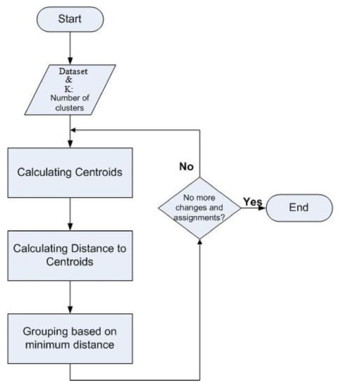
Figure 1. K-means Clustering Algorithm Flowchart.

• A set of data points.
• The number of clusters (K).

Then, it clusters data points into K clusters using a specific distance function. In the first round, some data points are chosen as centroids for each cluster randomly. Then, the distance between centroids and each data point is calculated. After that, data points are allocated in clusters based on the shortest distance from the selected data point to the closest centroid. After assigning all data points into clusters, centroids are recomputed again for each cluster. This is repeated until one of the stopping conditions takes place [13], these are:

• Data points are not reassigned to other clusters anymore (or minimum re-assignments); or
• Centroids are not recomputed anymore (or minimum change).

The output of this algorithm is a matrix of clusters indices (classes) for each data point in the provided dataset.

2.1. Number of Clusters (K)

There are many ways to recognize the most suitable number of clusters for a given data points the most well-known ones are: (1) elbow method [16] and (2) silhouette coefficients [17].

(1) Elbow method: elbow is a heuristic method that is used in cluster analysis for the purpose of determining the suitable number of clusters in a given dataset [16]. The output is a figure that shows the cut-off point of the curve (elbow) that indicates the optimal number of clusters. It is based on the percentage of variation by plotting the variation as a function of the number of clusters. In this sense, the optimal number of clusters reveals that adding more clusters will not provide much improvement to data/dataset modeling.

Many recent research works have used the elbow method, such as Bholowalia and Kumar [18], Syakur et al. [19], Abdullah et al. [20], Kong et al. [21], Thamrin and Wijayanto [22].

(2) Silhouette coefficients: silhouette is used to plot clustered data points. Silhouette is a graphical representation of data points in each cluster [17]. It shows whether data points are well-positioned in each cluster or not.

2.2. Motivation: K-Means in GIS

In our context, geolocations can be classified into different groups based on some topographical attribute similarities. The idea is to discover hidden patterns in large datasets by fetching data structure and finding similarities, such as elevation values. K-means clustering algorithm organizes data points (geolocations) into similar groups (clusters). Accordingly, data points in one cluster have similar topographical characteristics and data points in different clusters have different ones. Hence, data clustering comes with some challenges; this is related to finding the optimal number of groups (K) and the suitable distance function. In our context, a wrong number of classes (K) may create a misleading map and change the look of the map, and this conveys a wrong message, accordingly.

We applied the K-means clustering technique, based on the standard Euclidean distance, to present topographical data in a structured way. K-means data points are clustered into groups. Each group contains locations with similar features. In this paper, latitude and longitude are classified into different groups based on their elevation similarities.

We highlight the need for using the K-means algorithm in the field of GIS, as follows:

• K-means is an efficient algorithm that is suitable for handling large and complex datasets. It is capable of presenting data in a structured way. It is efficient at segmenting large datasets into groups based on some attribute similarities.
• K-means is used to discover hidden patterns in geospatial datasets. We argue that K-means is capable of making the correlation in elevation values explicit by finding structures and similarities in geospatial data in a given dataset.
• K-means improves data-retrieval potentials of our method by classifying elevation values into clusters. The resultant clusters facilitate the geospatial data interpretation and querying processes. Consequently, it will be easier to consider the context of location and features mapping in our interactive map.
• The K-means algorithm improves clustering accuracy. It improves the relevancy of the retrieved data from a given cluster. Moreover, it increases the recall metric by increasing the percentage of the relevant retrieved data in a given cluster.

3. Related Work

K-means clustering techniques have been used in different fields in the literature. This section presents a summary of some of the available research work in in literature that used K-means clustering techniques. The common factor in such works is to find similarities among data in a given dataset, but each work has its own domain and application.

Some work has used K-means clustering to find some structure in data that is related to geographical locations. For example, Tessa Anderson [23] presented a methodology for identifying road accident hotspots based on K-means using geographical information systems and kernel density estimation to study the spatial patterns of injury-related road accidents in London, UK. Specifically, Anderson employed the K-means clustering techniques to identify similar zones and to create a classification of road accident hotspots based on environmental data from 1999 to 2003. In line with Anderson’s work, Eghtesadifard et al. [24] present an integrated method for selecting the proper site for the disposing of solid waste based on K-means clustering and multi-criteria decision-making methods relying on GIS.

K-means clustering has been used in data analysis and prediction for the purpose of having preventive systems, in case of catastrophic events. For example, Annas and Rais [25] presented a preventive approach based on K-means clustering for mapping natural disaster-prone areas in Indonesia, by grouping such areas based on their similarities. In addition, they combined K-means and GIS to improve clusters visualization.

Burrough et al. [26] presented an approach for topoclimatic data classification using fuzzy K-means and allocation procedure to help in forest mapping. They built their approach based on data derived from 100 m gridded digital elevation models (DEMs). In line with Burrough, Lemenkova [27] presented an approach based on the K-means algorithm using R programming, for evaluating the similarities in a given geological data by analyzing some attributes, such as geology (sediment thickness), tectonics, volcanism, bathymetry, and geomorphology. Piloyan and Milan [28] presented a semi-automatic method based on K-means unsupervised classification to analyze geomorphometric features as landform elements in Armenia. They extracted data layers from DEM, then K-means algorithm was used for classifying landform.

Bholowalia and Kumar [18] developed a hybrid model based on the K-means clustering technique to produce a new cluster scheme for wireless sensor networks (WSNs).

In addition, K-means clustering was used in many other fields, such as system management [29], energy consumption [21], service selection [30,31], and technical debt management [32]. For instance, Brentan et al. [29] presented a hybrid approach to improve planning, operation, and management in water distribution systems based on K-means clustering. Recently, Kong et al. [21] proposed an energy consumption structure analysis method based on the K-means clustering algorithm. They used elbow and contour coefficient methods for data analysis. In line with the usage of the elbow method, Syakur et al. [19] presented an approach for customer mapping using K-means clustering. They employed K-means clustering techniques based on the elbow method for the purpose of grouping customer profiles to facilitate analysis and policy generation.

Furthermore, K-means clustering has been used in classifying cities based on certain factors. For example, Thamrin and Wijayanto [22] conducted a study for classifying cities based on the level of welfare. They used elbow, silhouette, and gap statistics to determine the optimal number of clusters. They conducted a comparison between soft and hard clustering based on a case study on welfare levels in cities in Java Island.

Recently, the COVID-19 pandemic led for the need of classifying countries, cities, and locations. Accordingly, Abdullah et al. [20] proposed an approach for clustering provinces in Indonesia based on COVID-19 data using the K-Means clustering technique for the purpose of clustering the risk of the COVID-19 pandemic in Indonesia. Their research aims to provide input to the government, in regard to making policies related to restrictions on community activities or other policies, to overcome the spread of COVID-19.

In this paper, we formulate the problem of topological data classification as a learning problem, and we approach it in terms of a learning algorithm. In particular, we integrate the K-means clustering algorithm with GIS data extraction from DEM raster images for the aim of uncovering relationships in the topological dataset for the area of Jordan, based on elevation similarities. We argue that this integration improves the mapping process in GIS. In addition, our method was implemented using Python and ArcGIS JavaScript API to unlock topological data potentials and visualize them accordingly.

4. Methodology

In this section, we present a method for geospatial data analysis based on elevation clustering using K-means algorithm and DEM raster image. Our method supports decision-making in GIS and enhances geospatial data retrieval and visualization processes by presenting topographical features on an interactive map.

We employed the K-means clustering algorithm and built on ArcGIS JavaScript API to unlock potentials in geospatial data analysis, decision-making, data retrieval, and mapping process in GIS. Our method consists of three main stages:

• Reading DEM raster images and extracting elevation using Python.
• Clustering elevation based on the K-means algorithm using Python.
• Retrieving and visualizing topographical features on an interactive map using ArcGIS API for JavaScript.

4.1. Data Collection and Preparation

The input of our method is a DEM raster image, which was obtained from [7]. First, we start by reading and interpreting topographic data from the acquired DEM raster image using Python.

Figure 2 represents the DEM raster image of the land around the area of Jordan. That is a digital representation of the bare ground topographic surface of Jordan, excluding trees, buildings, and any other surface objects.

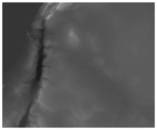
Figure 2. DEM raster image of the land around the area of Jordan (obtained from [7]).

Then, we customize the given DEM image as follows:

• The image is clipped according to the country shape of Jordan. Figure 3a represents the shape of the Jordan map.
  

  Figure 3. The clipped DEM raster image based on country shape of Jordan map (obtained from [7]). (a) Country shape of Jordan map. (b) Clipped DEM raster image of Jordan.
• The resultant (cropped) image is shown in Figure 3b. It represents the DEM raster image for Jordan map. According to Figure 3b, the elevation values vary from (−425) meters to 1718 m above sea level. The Dead Sea is the lowest point on earth [33]; this is demonstrated on the interactive map in the results section.

4.2. Dataset

We extract the needed topographical data from the cropped DEM raster image for Jordan (Figure 3b) using the Rasterio Python library (https://rasterio.readthedocs.io). The Rasterio library is a special Python library that assists in accessing raster geospatial data from a disk in either reading or writing mode.

In this research, we extracted elevation information from the DEM raster image in addition to latitude and longitude for each value (these values will be used as inputs for the next step). The extracted file contains 85,615 records and three attributes (latitude, longitude, and elevation value). The extracted values are then stored in a CSV file.

It is important to mention that we preprocessed the data. The original DEM raster image file was extremely huge, about 45 MB in size, and the original resolution was 6000 × 7000 pixels. Therefore, we downsampled the original file. The current file is 19.4 KB in size and the resolution is 373 × 345 pixels. The downsampling was performed using the wrap function from the GDAL library in Python. Comparing the downsampled data with the ground truth, the effect of downsampling was marginal.

4.3. K-Means Clustering

The K-means clustering technique is applied to the extracted data (from the previous step), to discover hidden patterns and produce the needed clusters based on elevation similarities. In this paper, we use K-means clustering for analyzing and investigating the structure of the topographical data in the area of Jordan, and then we visualize it accordingly.

K-means clustering was applied using the standard Euclidean as a distance function and the elbow method for determining the optimal number of clusters. Based on the elbow method, the optimal number of clusters is K = 4 (Figure 4). Figure 4 shows the cut-off point of the curve (elbow) that indicates the optimal number of clusters (K = 4). It reveals that adding more clusters will not provide much improvement to dataset modeling. We will discuss this in the results section in addition to other test cases for K = 5 and K = 6.

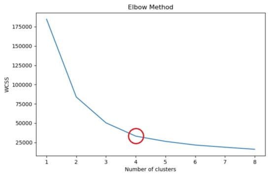
Figure 4. Elbow Chart.

4.4. Elevation Clusters

The output of the previous step is “elevation clusters”, which is a CSV file that contains clusters’ classes (numbers) for each elevation feature. This CSV file is used as an input for the next step accompanied by (1) elevation, (2) latitude, and (3) longitude values, respectively. It contains 85,615 records and four attributes (latitude, longitude, elevation value, and the cluster class number for each datum pixel).

4.5. Features Mapping

In the previous step, we employed K-means clustering to uncover hidden patterns in elevation values and improve the understanding of relationships among geospatial data. In this step, we process the CSV file, which contains elevation clusters and other geospatial data, to be plotted on our interactive map.

We built on the ArcGIS API using JavaScript and we implemented the features mapping process based on CSVLayer and MapView techniques from arcgis.com (https://developers.arcgis.com/javascript/latest/api-reference/esri-layers-CSVLayer.html) (accessed on 30 June 2021). CSVLayer is a point layer that facilitates building a map based on CSV files. We access elements from the CSV file and feed them as inputs to our interactive map building process based on geometry services. Specifically, elevation values are pinned onto our interactive map of Jordan as geometric objects using the MapView technique based on the latitude and longitude values for each data point.

The beauty of using the CSVLayer is that it plots each topographic feature and maps it to its corresponding geographic attributes; latitude and longitude, based on some built-in properties and templates.

4.6. Interactive Map Visualization

This is the final step, where the output is generated on an interactive map. We present topographic features on an interactive map by embedding them on a real online map. There are many benefits of using an interactive online map, such as accessing geospatial information easily and efficiently, querying topographic features, zoom in and out, getting details by clicking on a specific point on the map, etc. Interactive maps can reach a wide variety of users and can be modified to reflect changes in needs, requirements, and objectives.

We give a specific color for each point on the interactive map. As each cluster is represented by a class number. Each class is represented by a specific color on the interactive map. Accordingly, each elevation level in a specific cluster has a defined color. This will be explained furthermore in the results section.

5. Results and Discussion

We tested three values of K-number of clusters: K = 4, K = 5, and K = 6 respectively. In this section, we present the results of the three values of K to show the differences in clustering and to validate the optimal result (K = 4).

5.1. Elevation Clustering with K = 4

Based on the elbow method, the optimal number of clusters is k = 4 (Figure 4 in the methodology section). This implies that adding more clusters (classes on the map) will not add extra value to the clustering process, i.e., no more gain after K = 4. In this sense, the optimal decision is in favor of K = 4. Figure 5 represents our final interactive map, which has a layer that consists of four classes with four different colors for each class (class for each cluster).

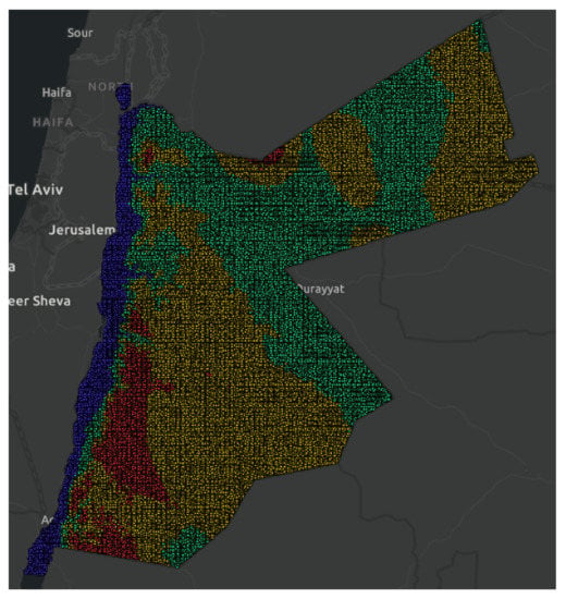
Figure 5. Elevation clustering in Jordan with k = 4.

In Figure 5, each cluster is represented by a class number. Each class is represented by a specific color on the map. Each color represents a specific level of elevation. Each elevation value belongs to a specific categorized range of values in a specific cluster.

Accordingly, the four classes are categorized as follows:

• Class 0: High elevation values in yellow color.
• Class 1: Very low elevation values in blue color.
• Class 2: Medium–high elevation values in green color.
• Class 3: Very high elevation values in red color.

Accordingly, the elevation values range in each cluster, with k = 4 categorized as follows:

• Cluster number 0: elevation values range = 758 to 1039.
• Cluster number 1: elevation values range = (−425) to 286.
• Cluster number 2: elevation values range = 287 to 757.
• Cluster number 3: elevation values range = 1040 to 1718.

Table 1 presents the details of the cluster elevation ranges and descriptions when K = 4. The first column presents the cluster number. The second column presents the description of elevation values in each cluster. The third column presents the descriptive color on the map. Finally, the fourth and fifth columns present the lowest and highest values of elevation in each cluster, respectively.

Table 1. Clusters’ elevation ranges and descriptions with K = 4.

Cluster	Description	Colour	Lowest	Highest
0	High	Yellow	758	1039
1	Very Low	Blue	−425	286
2	Medium High	Green	287	757
3	Very High	Red	1040	1718

Table 2 presents a sample of longitude and latitude points on the map, accompanied by a specific elevation value, either the lowest or the highest value in each cluster when K = 4.

Table 2. Elevation—lowest and highest value–longitude and latitude samples in each cluster with K = 4.

Class	L/H	Elevation	Longitude	Latitude
0	Lowest	758	38.71458333	33.32541667
0	Highest	1039	35.76458333	32.37541667
1	Lowest	−425	35.41458333	31.53541667
1	Highest	286	35.67458333	32.29541667
2	Lowest	287	35.49458333	30.63541667
2	Highest	757	38.67458333	33.28541667
3	Lowest	1040	37.00458333	32.33541667
3	Highest	1718	35.50458333	30.37541667

5.2. Elevation Clustering with K = 5

Figure 6 shows the map that represents elevation values clustering based on K-means clustering with K = 5 (for comparison). The five classes are categorized as follows:

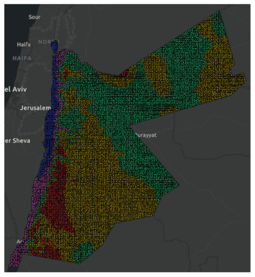
Figure 6. Elevation clustering in Jordan with k = 5.

• Class 0: Medium–high elevation values in green color.
• Class 1: Very low elevation values in blue color.
• Class 2: High elevation values in yellow color.
• Class 3: Very high elevation values in red color.
• Class 4: Low elevation values in pink color.

The elevation values range in each cluster with k = 5 is categorized as follows:

• Cluster number 0: elevation values range = 411 to 772.
• Cluster number 1: elevation values range = (−425) to (−72).
• Cluster number 2: elevation values range = 773 to 1053.
• Cluster number 3: elevation values range = 1054 to 1718.
• Cluster number 4: elevation values range = (−71) to 410.

Table 3 presents the details of the cluster elevation ranges and descriptions when K = 5. Table 4 presents a sample of longitude and latitude points on the map, accompanied by a specific elevation value, either the lowest or the highest value in each cluster when K = 5.

Table 3. Clusters information with K = 5.

Cluster	Description	Color	Lowest	Highest
0	Medium High	Green	411	772
1	Very Low	Blue	−425	−72
2	High	Yellow	773	1053
3	Very High	Red	1054	1718
4	Low	Pink	−71	410

Table 4. Elevation—lowest and highest value–longitude and latitude in each cluster with K = 5.

Class	L/H	Elevation	Longitude	Latitude
0	Lowest	411	35.93458333	32.70541667
0	Highest	772	37.52458333	32.65541667
1	Lowest	−425	35.41458333	31.53541667
1	Highest	−72	35.53458333	31.08541667
2	Lowest	773	38.65458333	33.28541667
2	Highest	1053	35.79458333	32.37541667
3	Lowest	1054	36.95458333	32.29541667
3	Highest	1718	35.50458333	30.37541667
4	Lowest	−71	35.75458333	32.73541667
4	Highest	410	35.70458333	32.48541667

5.3. Elevation Clustering with K = 6

Figure 7 shows the map that represents elevation values clustering based on K-means clustering with K = 6 (for comparison). The six classes are categorized as follows:

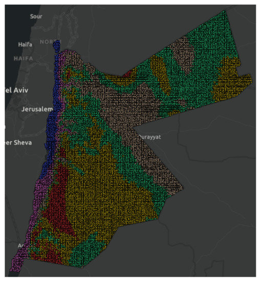
Figure 7. Elevation clustering in Jordan with k = 6.

• Class 0: High elevation values in yellow color.
• Class 1: Very low elevation values in blue color.
• Class 2: Very high elevation values in red color.
• Class 3: Low high elevation values in beige color.
• Class 4: Low elevation values in pink color.
• Class 5: Medium–high elevation values in green color.

The elevation values range in each cluster with k = 6 is categorized as follows:

• Cluster number 0: elevation values range = 838 to 1086.
• Cluster number 1: elevation values range = (−425) to (−89).
• Cluster number 2: elevation values range = 1087 to 1718.
• Cluster number 3: elevation values range = 365 to 681.
• Cluster number 4: elevation values range = (−88) to 364.
• Cluster number 5: elevation values range = 682 to 837.

Table 5 presents the details of the cluster elevation ranges and descriptions when K = 6. Table 6 presents a sample of longitude and latitude points on the map, accompanied by a specific elevation value, either the lowest or the highest value in each cluster when K = 6.

Table 5. Clusters information with K = 6.

Cluster	Description	Color	Lowest	Highest
0	High	Yellow	838	1086
1	Very Low	Blue	−425	−89
2	Very High	Red	1087	1718
3	Low High	Beige	365	681
4	Low	Pink	−88	364
5	Medium High	Green	682	837

Table 6. Elevation—lowest and highest value–longitude and latitude in each cluster with K = 6.

Class	L/H	Elevation	Longitude	Latitude
0	Lowest	838	38.81458333	32.63541667
0	Highest	1086	35.75458333	31.08541667
1	Lowest	−425	35.41458333	31.49541667
1	Highest	−89	35.61458333	31.94541667
2	Lowest	1087	35.74458333	30.47541667
2	Highest	1718	35.50458333	30.37541667
3	Lowest	365	35.79458333	32.62541667
3	Highest	681	38.11458333	32.82541667
4	Lowest	−88	35.61458333	31.46541667
4	Highest	364	35.03458333	29.37541667
5	Lowest	682	38.06458333	32.98541667
5	Highest	837	38.83458333	32.64541667

5.4. Interactive Data Visualization and Retrieval

Finally, we deal with elements from CSV files as geometric objects and feed them as inputs to our interactive map. The interactive map is customized based on data from the CVS file. This will add value in terms of geospatial data retrieval, querying, and analysis. This increases the quality of responses to users’ actions by presenting the needed content as interactive features. Rather than a static map, the interactive map improves the quality (look and feel) of the retrieved geospatial information and reveals topographical data correlation instantly.

Figure 8 represents the interactive map of Jordan when elevation is clustered into four classes. Figure 9 represents a sample of some interactive features on the map, which allow users to access the map using different scales. Zoom in and zoom out indicate increasing and decreasing the scale of the map, respectively. Figure 10 represents the “more details” view whenever the user clicks on any geolocation pixel on the map.

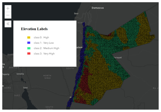
Figure 8. Elevation clustering in Jordan with k = 4.

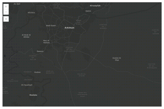
Figure 9. Zoom in/out feature.

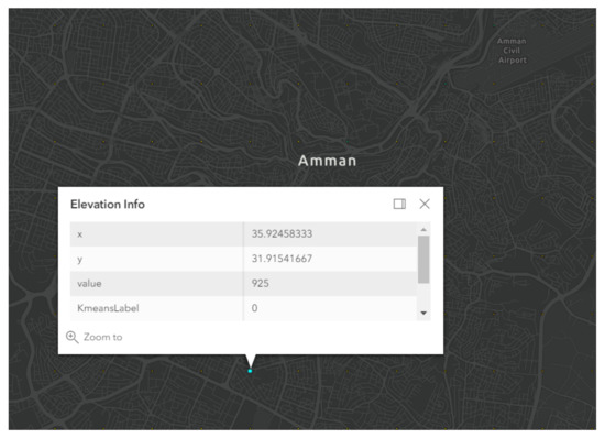
Figure 10. More details feature.

6. Evaluation

Silhouette is one of the most popular and effective measures for evaluating clustering validity when comparing different values of K [34]. Silhouette coefficients are used to test whether if data points are well clustered. It quantifies which data points lie well within the cluster and which ones are merely somewhere in between clusters.

Figure 11 represents the silhouette plot for elevation clusters with k = 4. Figure 12 represents the average silhouette value when k = 4. The x-axis represents the silhouette width S(i). It quantifies how well data points are clustered based on the following values:

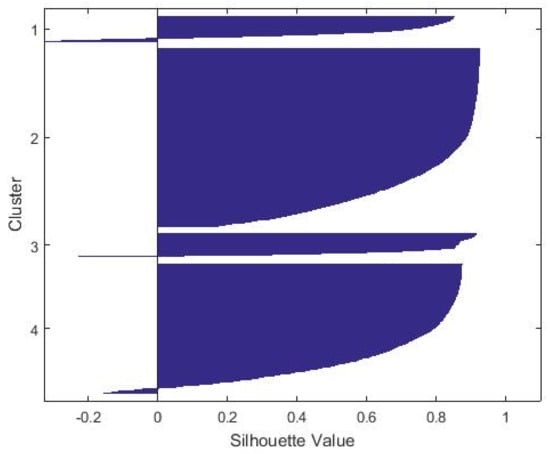
Figure 11. Silhouette diagram for elevation clusters when k = 4.

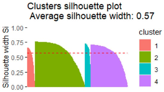
Figure 12. Average silhouette value when k = 4.

• If the S(i) value is close to 1, it means that the sample data are “well-clustered” and each datum point is assigned to an appropriate cluster.
• If the S(i) value is almost zero, it means that the sample data could be assigned to another cluster and the sample data lie equally far away from both clusters.
• If the S(i) value is close to −1, it means that the sample data are “misclassified” and is merely somewhere in between the clusters.

7. Conclusions and Future Work

We presented a method for topographical data clustering in Jordan, based on elevation similarities using the K-means algorithm. We also presented a novel interactive map for enhancing geospatial data retrieval and visualization by presenting topographical features on it and responding to user actions by presenting the needed content as interactive features. We highlighted the need for using the K-means clustering technique in GIS applications and how this adds value to the map visualization and interactivity processes.

Our method provided insights into data analysis by discovering hidden patterns in geospatial data and topographical features. It also facilitated decision-making by clustering geospatial data into homogeneous groups. It revealed the optimal clustering of elevation values for the area of Jordan based on the DEM raster image. The goal of clustering is achieved by exposing homogeneous elevation values on an interactive map and enhancing data retrieval and visualization accordingly. The results show the final output as a colored interactive map and prove that the optimal clustering decision is in favor of K = 4, i.e., four clusters (classes).

In this research, we crafted the methodology to deal with elevation values from DEM and we will build on it in future work to deal with the aspect and slope. More research is currently underway, seeking to utilize the usage of DEM raster images and how to quantify several key topographic metrics from DEMs, such as slope, aspect, flow direction, flow accumulation area, topographic index, etc. We focus on extracting slope and aspect from DEM to support decision-making and geospatial data analysis in many fields, such as agriculture, roads and bridges, engineering, highway construction, maintenance, management, etc. We argue that presenting topographical features on an interactive map unlocks the potential of geospatial data analysis and retrieval.

References

- Fujisada, H.; Bailey, G.B.; Kelly, G.G.; Hara, S.; Abrams, M.J. Aster dem performance. IEEE Trans. Geosci. Remote Sens. 2005, 43, 2707–2714. [Google Scholar] [CrossRef]
- Toppe, R. Terrain Models: A Tool for Natural Hazard Mapping; IAHS: Wallingford, UK, 1987; Volume 162. [Google Scholar]
- Archuleta, C.A.M.; Constance, E.W.; Arundel, S.T.; Lowe, A.J.; Mantey, K.S.; Phillips, L.A. The National Map Seamless Digital Elevation Model Specifications; Technical Report; US Geological Survey: Washington, DC, USA, 2017.
- Patterson, T. DEM Manipulation and 3-D Terrain Visualization: Techniques Used by the U.S. National Park Service. Cartogr. Int. J. Geogr. Inf. Geovis. 2001, 38, 89–101. [Google Scholar] [CrossRef]
- Bernhardsen, T. Geographic Information Systems: An Introduction; John Wiley & Sons: Hoboken, NJ, USA, 2002. [Google Scholar]
- Garrard, C. Geoprocessing with Python; Simon and Schuster: New York, NY, USA, 2016. [Google Scholar]
- Bataineh, S. Jordan Digital Elevation Model. JUST GIS Lab./Civ. Eng. 2021. Available online: https://www.just.edu.jo/FacultiesandDepartments/FacultyofEngineering/Departments/CivilEngineering/Pages/gis_maps.aspx (accessed on 28 June 2012).
- Pan, F.; Xi, X.; Wang, C. A MATLAB-based digital elevation model (DEM) data processing toolbox (MDEM). Environ. Model. Softw. 2019, 122, 104566. [Google Scholar] [CrossRef]
- Fisher, P.F.; Tate, N.J. Causes and consequences of error in digital elevation models. Prog. Phys. Geogr. 2006, 30, 467–489. [Google Scholar] [CrossRef]
- Balasubramanian, A. Digital Elevation Model (DEM) in GIS; University of Mysore: Mysuru, India, 2017. [Google Scholar]
- Xiong, L.; Wang, G.; Wessel, P. Anti-aliasing filters for deriving high-accuracy DEMs from TLS data: A case study from Freeport, Texas. Comput. Geosci. 2017, 100, 125–134. [Google Scholar] [CrossRef]
- Woodruff, S.; Vitro, K.A.; BenDor, T.K. GIS and Coastal Vulnerability to Climate Change; Elsevier: Amsterdam, The Netherlands, 2018. [Google Scholar]
- MacQueen, J. Some methods for classification and analysis of multivariate observations. In Proceedings of the Fifth Berkeley Symposium on Mathematical Statistics and Probability, Oakland, CA, USA; 1967; Volume 1, pp. 281–297. [Google Scholar]
- Ahmed, M.; Seraj, R.; Islam, S.M.S. The k-means Algorithm: A Comprehensive Survey and Performance Evaluation. Electronics 2020, 9, 1295. [Google Scholar] [CrossRef]
- Dasgupta, S.; Freund, Y. Random Projection Trees for Vector Quantization. Inf. Theory IEEE Trans. 2009, 55, 3229–3242. [Google Scholar] [CrossRef] [Green Version]
- Thorndike, R.L. Who belongs in the family? Psychometrika 1953, 18, 267–276. [Google Scholar] [CrossRef]
- Rousseeuw, P.J. Silhouettes: A graphical aid to the interpretation and validation of cluster analysis. J. Comput. Appl. Math. 1987, 20, 53–65. [Google Scholar] [CrossRef] [Green Version]
- Bholowalia, P.; Kumar, A. Article: EBK-Means: A Clustering Technique based on Elbow Method and K-Means in WSN. Int. J. Comput. Appl. 2014, 105, 17–24, Full text available. [Google Scholar]
- Syakur, M.A.; Khotimah, B.K.; Rochman, E.M.S.; Satoto, B.D. Integration K-Means Clustering Method and Elbow Method For Identification of The Best Customer Profile Cluster. IOP Conf. Ser. Mater. Sci. Eng. 2018, 336, 012017. [Google Scholar] [CrossRef] [Green Version]
- Abdullah, D.; Susilo, S.; Ahmar, A.S.; Rusli, R.; Hidayat, R. The application of K-means clustering for province clustering in Indonesia of the risk of the COVID-19 pandemic based on COVID-19 data. Qual. Quant. 2021, 1–9. [Google Scholar] [CrossRef] [PubMed]
- Kong, W.; Wang, Y.; Dai, H.; Zhao, L.; Wang, C. Analysis of energy consumption structure based on K-means clustering algorithm. In Proceedings of the E3S Web 7th International Conference on Energy Science and Chemical Engineering, Dali, China, 21–23 May 2021; Volume 267, p. 01054. [Google Scholar]
- Thamrin, N.; Wijayanto, A.W. Comparison of Soft and Hard Clustering: A Case Study on Welfare Level in Cities on Java Island: Analisis cluster dengan menggunakan hard clustering dan soft clustering untuk pengelompokkan tingkat kesejahteraan kabupaten/kota di pulau Jawa. Indones. J. Stat. Its Appl. 2021, 5, 141–160. [Google Scholar] [CrossRef]
- Anderson, T.K. Kernel density estimation and K-means clustering to profile road accident hotspots. Accid. Anal. Prev. 2009, 41, 359–364. [Google Scholar] [CrossRef] [PubMed]
- Eghtesadifard, M.; Afkhami, P.; Bazyar, A. An integrated approach to the selection of municipal solid waste landfills through GIS, K-Means and multi-criteria decision analysis. Environ. Res. 2020, 185, 109348. [Google Scholar] [CrossRef] [PubMed]
- Annas, S.; Rais, Z. k-Means and GIS for Mapping Natural Disaster Prone Areas in Indonesia. In Proceedings of the 7th Mathematics, Science, and Computer Science Education International Seminar, MSCEIS 2019, Bandung, India, 12 October 2019. [Google Scholar]
- Burrough, P.A.; Wilson, J.P.; Van Gaans, P.F.; Hansen, A.J. Fuzzy k-means classification of topo-climatic data as an aid to forest mapping in the Greater Yellowstone Area, USA. Landsc. Ecol. 2001, 16, 523–546. [Google Scholar] [CrossRef]
- Lemenkova, P. K-means Clustering in R Libraries {cluster} and {factoextra} for Grouping Oceanographic Data. Int. J. Inform. Appl. Math. 2019, 2, 1–26. [Google Scholar]
- Piloyan, A.; Konečnỳ, M. Semi-automated classification of landform elements in Armenia based on SRTM DEM using k-means unsupervised classification. Quaest. Geogr. 2017, 36, 93–103. [Google Scholar] [CrossRef] [Green Version]
- Brentan, B.; Meirelles, G.; Luvizotto, E., Jr.; Izquierdo, J. Hybrid SOM+ k-Means clustering to improve planning, operation and management in water distribution systems. Environ. Model. Softw. 2018, 106, 77–88. [Google Scholar] [CrossRef]
- Alzaghoul, E.; Bahsoon, R. Economics-driven approach for managing technical debt in cloud-based architectures. In Proceedings of the IEEE/ACM 6th International Conference on Utility and Cloud Computing, Dresden, Germany, 9–12 December 2013; pp. 239–242. [Google Scholar]
- Alzaghoul, E.; Bahsoon, R. Evaluating technical debt in cloud-based architectures using real options. In Proceedings of the 23rd Australian Software Engineering Conference, Milsons Point, Australia, 7–10 April 2014; pp. 1–10. [Google Scholar]
- Alzaghoul, E. Value-and Debt-Aware Selection and Composition in Cloud-Based Service-Oriented Architectures Using Real Options. Ph.D. Thesis, University of Birmingham, Birmingham, UK, 2015. [Google Scholar]
- McCoy, J.; Group, G. Geo-Data: The World Geographical Encyclopedia; Gale Virtual Reference Library, Thomson-Gale: Farmington Hills, MI, USA, 2003. [Google Scholar]
- Wang, F.; Franco-Penya, H.H.; Kelleher, J.D.; Pugh, J.; Ross, R. An Analysis of the Application of Simplified Silhouette to the Evaluation of k-means Clustering Validity. In Machine Learning and Data Mining in Pattern Recognition; Perner, P., Ed.; Springer International Publishing: Cham, Switzerland, 2017; pp. 291–305. [Google Scholar]
Publisher’s Note: MDPI stays neutral with regard to jurisdictional claims in published maps and institutional affiliations. |
© 2021 by the authors. Licensee MDPI, Basel, Switzerland. This article is an open access article distributed under the terms and conditions of the Creative Commons Attribution (CC BY) license (https://creativecommons.org/licenses/by/4.0/).