Measuring Technological Change through an Extended Structural Decomposition Analysis: An Application to EU-28 Primary Sectors (2010–2015)

Abstract

This paper addresses the input–output structural decomposition for an economic analysis. The objective is to determine the causes of changes in production in these sectors with a particular focus on disaggregating the technological change by distribution factors associated with a specific normalization of the Leontief inverse. In calculating the net multipliers, an attempt was made to exclude each sectors’ own consumption in a satisfactory manner. However, the treatment of own consumption when introducing a time factor requires further investigation to avoid questionable measurements. An empirical application is presented regarding agriculture, forestry, and fishing sectors in six EU-28 countries (Austria, Belgium, France, Germany, Italy, and Spain) over the 2010–2015 period. In general, a typical characteristic of primary sectors is the accumulation of a significant amount of their own consumption, facilitated by the design of their own symmetric accounting methods. Therefore, attention is focused on these sectors so as to reveal possible analysis techniques that will provide nuance or validate existing techniques.

1. Introduction

Structural decomposition analysis (SDA) is a practical tool that allows us to quantify the causes of changes in a wide range of variables, such as economic growth, energy consumption, and labor demand, etc. Input–output (IO) SDA is usually defined as the study of economic change by comparing a series of static changes in the main variables of an IO model (Rose and Chen 1991).

The most traditional and straightforward SDA usually concerns three drivers of structural change: technological changes relating to the effects caused by changes in the Leontief inverse; changes in final demand (which are usually sub-divided into changes in levels and the composition of final demand); and the interaction or combination of both (Miller and Blair 2009). There is extensive related literature (see Hoekstra and Van Der Bergh 2003) using this methodology in various empirical studies to analyze production changes (Fujimagari 1989), changes in employment (Forssell 1990; Han 1995), and labor productivity. However, it is chiefly applied to energy consumption, CO₂ emissions, and other environmental issues (Casler and Rose 1998; Chen and Wu 1994; Han and Lakshmanan 1994; Jacobsen 2000; Mukhopadhyay and Chakraborty 1999). There have also been numerous developmental proposals for the theoretical approach to the model (Chen and Wu 2008; Dietzenbacher and Los 1998; Rose and Casler 1996; Sonis et al. 1996; Wang et al. 2014). In other words, SDA is an appropriate methodology for analyzing the driving forces behind changes in economic, energy, and environmental indicators.

In general, SDA formulas have been modified by new ways of decomposing the factors. However, less attention has been paid to changes in the Leontief inverse (Wood and Lenzen 2009; Muradov 2021). Therefore, decomposing structural change by the (overall) effect caused by the sectors’ own consumption is proposed. A specific normalization criterion, by rows and columns of the model, is thus applied.

SDA is also used in the field of agricultural economics, especially regarding environmental issues. Studies are available at the EU level. For example, in Italy, over the 1999–2006 period, the analysis was applied to energy and environmental outputs to determine the impact of energy intensity and emissions, the Leontief effect, and the final demand effect on changes in certain volumes, concluding that ‘agriculture, hunting and forestry’ are among the main sectors affecting atmospheric emissions (Cellura et al. 2012). The analysis was used to see how changes in final demand and technology affected variations in water use for different crops in the EU. The results revealed that major crop producers increased their water use mainly due to technology changes (Gerveni et al. 2020). Intrinsic reasons for the increase in global consumption-based GHG emissions (1995–2009) were also analyzed, with agriculture playing an important role in developing countries (Liu et al. 2019). SDA was also applied to examine water use changes in agricultural production in the United States (1995–2010). It revealed an overall decrease in water use in the production of all crops due to more efficient irrigation systems (Avelino and Dall’erba 2020). However, there is no doubt that the largest number of SDAs conducted have focused on China, both nationwide and at the provincial level. This method was used to determine drivers of metal consumption in China (1997–2015) in agriculture, industry, construction, and services (Song et al. 2019), and to estimate energy-related CO₂ emissions and structural emissions reductions in Chinese agriculture (2007–2017). It was found, among other things, that increasing agricultural demand across the industrial system fostered the growth of these emissions (Yu et al. 2020). Other similar provincial-level papers concerning China using SDA, sometimes in combination with complementary techniques, include the works of Cai et al. (2019); Fang and Yang (2021); Feng et al. (2017); D. Li et al. (2020); W. Li et al. (2020); X. Li et al. (2020); Liu and Liang (2017); Qian et al. (2018); Supasa et al. (2017); Wang et al. (2016); Zhi et al. (2014); and Xu et al. (2017). Studies of a socio-economic nature are uncommon, although they do exist. In China, for example, the sources of employment growth were analyzed using this method. It was found that the contribution of exports to job creation increased significantly, especially in agriculture (Doan and Long 2019). The present investigation aims to fill this gap in literature using SDA to measure technological change.

The changes (in terms of output) in the primary sectors of the six countries of EU-28 between 2010 and 2015 are analyzed empirically, based on symmetric IO tables (total flows). A relatively short period was chosen, one that was characterized by stagnation and even by a deterioration in macro-economic indicators. Therefore, it is to be expected that these sectors did not experience significant changes in their production structure. At the same time, price changes during this period were not significant, yet deflation, based on 2010, was applied to the flows. The change in output is largely driven by final demand behavior and can be broken down by its components. It is now necessary to see to what extent the technological change (the second cause of change) can be broken down according to the IO logic. The total effects are calculated based on the effect of final demand and direct and indirect requirement effects. This idea is embodied in the Leontief inverse construction, so it is amenable to decomposition by distribution coefficients (associated with a particular normalization) corresponding to this logic.

In calculating net IO multipliers, the goal is to exclude these sectors’ own consumption from the calculation properly. Primary sectors tend to accumulate a large amount of own consumption in their cost structures, and the development of symmetric accounting in itself favors this situation. While extrapolating this recommended filtering of multipliers to the notion of technological change, attention should be focused on these sectors to reveal possible analytical means of refining or enhancing existing ones.

2. Methodology

SDA and its extensions have identified various sources of change in both the economy and its production sectors. To achieve the disaggregation of technological change, a specific modification of the SDA is required. Decompositions of the Leontief inverse vary, but the point is to look for the right one to achieve the stated goal.

2.1. Normalization of the Leontief Inverse Matrix

The open demand model, or Leontief model, can be expressed as follows:

$$x={(I-A)}^{-1}y=Cy,$$

(1)

where $x$ is the output vector, ${(I-A)}^{-1}$ is the Leontief inverse matrix—which is further simplified as C—and $y$ is the net import final demand vector. Here, $A$ is a matrix of technical coefficients (total flows). Its generic element, denoted by $a_{ij}$, represents the contribution of sector, $i$, per unit of output of sector, $j$. Furthermore, the economy studied is considered to be broken down into n sectors.

The following is probably the most traditional way to present the Leontief inverse matrix, as follows:

$$C=I+A+A^2+\cdots$$

(2)

where the generic element ${\alpha }_{ij}\left(i,j=1,\dots ,n\right)$ is presented as follows:

$$\{\begin{array}{c}1+a_{ij}+{{\displaystyle \sum }}_{k=1}^n{a}_{ik}{a}_{kj}+{{\displaystyle \sum }}_{k_1=1}^n{{\displaystyle \sum }}_{k_2=1}^n{a}_{i{k}_1}{a}_{k_1{k}_2}{a}_{k_{2}j}+\cdots ,\left(i=j\right)\\ a_{ij}+{{\displaystyle \sum }}_{k=1}^n{a}_{ik}{a}_{kj}+{{\displaystyle \sum }}_{k_1=1}^n{{\displaystyle \sum }}_{k_2=1}^n{a}_{i{k}_1}{a}_{k_1{k}_2}{a}_{k_{2}j}+\cdots ,\left(i\ne j\right)\end{array}$$

(3)

For alternative decompositions of $C,$ a diagonal matrix, $\widehat{D}$, is constructed with the elements of the main diagonal, $C$, which are the sum of the elements of the main diagonals of these $I,A,A^2,\cdots ,A^n,\cdots$ matrices. In analytical terms, such a diagonal matrix can be expressed as follows:

$$\widehat{D}=I+diag\left(A\right)+diag\left(A^2\right)+\cdots +diag\left(A^n\right)+\cdots ,$$

(4)

where the generic element is presented as follows:

$$d_i={\alpha }_{ii}=1+a_{ii}+{{\displaystyle \sum }}_{k=1}^n{a}_{ik}{a}_{ki}+{{\displaystyle \sum }}_{k_1=1}^n{{\displaystyle \sum }}_{k_2=1}^n{a}_{i{k}_1}{a}_{k_1{k}_2}{a}_{k_{2}i}+\cdots .$$

(5)

From here, one can derive the decomposition of the Leontief inverse matrix, as follows:

$$\begin{gathered} C=\widehat{D}{\widehat{D}}^{-1}C=\left(I+diag\left(A\right)+diag\left(A^2\right)+\cdots +diag\left(A^n\right)+\cdots \right){\widehat{D}}^{-1}C \\ ={\widehat{D}}^{-1}C+diag\left(A\right){\widehat{D}}^{-1}C+diag\left(A^2\right){\widehat{D}}^{-1}C+\cdots +diag\left(A^n\right){\widehat{D}}^{-1}C+\cdots \end{gathered}$$

(6)

In this decomposition, normalization is produced by the rows of the $C$ matrix, as follows:

$${\tilde{C}}^f\left(row\right)={\widehat{D}}^{-1}C=\left(\begin{array}{cccc}1& \frac{{\alpha }_{12}}{{\alpha }_{11}}& \cdots & \frac{{\alpha }_{1n}}{{\alpha }_{11}}\\ \frac{{\alpha }_{21}}{{\alpha }_{22}}& 1& \cdots & \frac{{\alpha }_{2n}}{{\alpha }_{22}}\\ ⋮& ⋮& \ddots & ⋮\\ \frac{{\alpha }_{n1}}{{\alpha }_{nn}}& \frac{{\alpha }_{n2}}{{\alpha }_{nn}}& \cdots & 1\end{array}\right).$$

(7)

This normalization criterion was applied, albeit partially (Jeong 1982, 1984), to the direct and indirect input demand matrix and $\left(C-I\right)$, and was later used by Gim and Kim (1998) for this matrix in its entirety. In this way, the $C$ elements are adjusted by row according to the value of the main diagonal (associated with the production branch); that is, the elements are amenable to be used for the quantification of net multipliers and are linked, from a methodological point of view, to the hypothetical extraction method.

Another normalization of $C$ is given by the following:

$${\tilde{C}}^g\left(row\right)=\left(I-{\widehat{D}}^{-1}\right)C=\left(\begin{array}{cccc}{\alpha }_{11}-1& \frac{{\alpha }_{11}-1}{{\alpha }_{11}}{\alpha }_{12}& \cdots & \frac{{\alpha }_{11}-1}{{\alpha }_{11}}{\alpha }_{1n}\\ \frac{{\alpha }_{22}-1}{{\alpha }_{22}}{\alpha }_{21}& {\alpha }_{22}-1& \cdots & \frac{{\alpha }_{22}-1}{{\alpha }_{22}}{\alpha }_{2n}\\ ⋮& ⋮& \ddots & ⋮\\ \frac{{\alpha }_{nn}-1}{{\alpha }_{nn}}{\alpha }_{n1}& \frac{{\alpha }_{nn}-1}{{\alpha }_{nn}}{\alpha }_{n2}& \cdots & {\alpha }_{nn}-1\end{array}\right).$$

(8)

This matrix is constructed in a similar way to (7), except that the transformations are conditioned by the effects provided by $\left({\alpha }_{ii}-1\right),i=1,2\dots ,n;$ i.e., the direct effect of final demand on the multipliers is excluded.

Next, one can see the role that normalization by $C$ rows plays in the model itself. Thus, if one considers (1), and if a particular modification is applied, the following distribution is found:

$$\begin{array}{ll}x& =Cy=ICy=\left({\widehat{D}}^{-1}+I-{\widehat{D}}^{-1}\right)Cy\\ & =\left[{\widehat{D}}^{-1}C+\left(I-{\widehat{D}}^{-1}\right)C\right]y={\widehat{D}}^{-1}Cy+\left(I-{\widehat{D}}^{-1}\right)Cy,\end{array}$$

(9)

in short, it can be seen that:

$$x={\tilde{C}}^f\left(row\right)y+{\tilde{C}}^g\left(row\right)y.$$

(10)

Therefore, the generic element $C$ is broken down by two (or more) distribution factors, as follows:

$${\alpha }_{ij}=\frac{1}{{\alpha }_{ii}}{\alpha }_{ij}+\frac{{\alpha }_{ii}-1}{{\alpha }_{ii}}{\alpha }_{ij}.$$

(11)

Disaggregating ${\alpha }_{ij}$ based on the effect produced by an increase in one unit of final demand and the other effects (occurring at different stages of production) that make up the ${\alpha }_{ii}$ normalizing element. Thus, a production sector with high levels of own consumption will generally lead to normalizing elements with a higher value. As a result, the distribution coefficient $\frac{1}{{\alpha }_{ii}}$ decreases and (simultaneously) the $\frac{{\alpha }_{ii}-1}{{\alpha }_{ii}}$ coefficient increases. The opposite is true in sectors with a low own consumption. This means that the calculation of net multipliers varies by sector. Of course, the $\frac{{\alpha }_{ii}-1}{{\alpha }_{ii}}$ factor can be further broken down according to (5), at least by distinguishing between direct and indirect requirements: $\frac{a_{ii}}{{\alpha }_{ii}}$ and $\frac{{\alpha }_{ii}-\left(1+a_{ii}\right)}{{\alpha }_{ii}}.$

The first equation of system (10) can be considered based on the following example:

$$x_1=\left[y_1+\frac{{\alpha }_{12}}{{\alpha }_{11}}{y}_2+\dots +\frac{{\alpha }_{1n}}{{\alpha }_{11}}{y}_n]+[\left({\alpha }_{11}-1\right)y_1+\frac{{\alpha }_{11}-1}{{\alpha }_{11}}{\alpha }_{12}{y}_2+\dots \frac{{\alpha }_{11}-1}{{\alpha }_{11}}{\alpha }_{1n}{y}_n\right].$$

(12)

Another possible transformation of $C$ is as follows:

$$\begin{array}{ll}C& =C\widehat{D}{\widehat{D}}^{-1}=C\left(I+diag\left(A\right)+diag\left(A^2\right)+\cdots +diag\left(A^n\right)+\cdots \right){\widehat{D}}^{-1}\\ & =C{\widehat{D}}^{-1}+Cdiag\left(A\right){\widehat{D}}^{-1}+Cdiag\left(A^2\right){\widehat{D}}^{-1}+\cdots +Cdiag\left(A^n\right){\widehat{D}}^{-1}+\cdots \end{array}$$

(13)

Therefore, normalization by columns in the Leontief inverse matrix is found in a similar way, as follows:

$${\tilde{C}}^f\left(col\right)=C{\widehat{D}}^{-1}$$

(14)

and

$${\tilde{C}}^g\left(col\right)=C\left(I-{\widehat{D}}^{-1}\right).$$

(15)

This normalization was applied to $\left(C-I\right)$ by Gim and Kim (2005), and Miller and Blair (2009) applied it directly to $C$.

Similarly, one can see the role of normalization by columns in the following model:

$$\begin{array}{ll}x& =Cy=CIy=C\left({\widehat{D}}^{-1}+I-{\widehat{D}}^{-1}\right)y\\ & =C{\widehat{D}}^{-1}y+C\left(I-{\widehat{D}}^{-1}\right)y={\tilde{C}}^f\left(col\right)y+{\tilde{C}}^g\left(col\right)y.\end{array}$$

(16)

This way, two alternative distributions for the Leontief inverse matrix are obtained. Additionally:

$$C={\tilde{C}}^f\left(row\right)+{\tilde{C}}^g\left(row\right)={\tilde{C}}^f\left(col\right)+{\tilde{C}}^g\left(col\right).$$

(17)

It is mathematically possible to use a combination of two matrix normalization methods, as follows:

$$2x=\left[{\tilde{C}}^f\left(row\right)y+{\tilde{C}}^g\left(row\right)y]+[{\tilde{C}}^f\left(col\right)y+{\tilde{C}}^g\left(col\right)y\right].$$

(18)

To conclude that:

$$x=0.5\left[{\tilde{C}}^f\left(row\right)+{\tilde{C}}^f\left(col\right)\left]y+0.5\right[{\tilde{C}}^g\left(row\right)+{\tilde{C}}^g\left(col\right)\right]y,$$

(19)

Which, in a shortened form, the demand model can be expressed as follows:

$$x={\tilde{C}}^{f}y+{\tilde{C}}^{g}y.$$

(20)

Thus, the demand model, expressed in this way, breaks down the overall impact into two factors; it quantifies a sector’s weight in terms of its relative external contribution to market interdependence, and it reproduces the size of the corresponding economy.

2.2. Structural Decomposition Analysis

The purpose of structural decomposition analysis is to isolate the main sources of change in the economy and its production sectors over a certain period. More specifically, it is a matter of detecting what part of the economic change between two points in time is related to technological change factors or productive efficiency, and what part is due to changes in final demand.

Thus, the increase in output between year 0 and year 1 is as follows:

$$\mathsf{\Delta }x=C_1{y}_1-C_0{y}_0,$$

(21)

Given that $y_1=y_0+\mathsf{\Delta }y$ and $C_1=C_0+\mathsf{\Delta }C,$ it is possible to express the above in different ways.

Such as:

$$\mathsf{\Delta }x=C_1\left(y_0+\mathsf{\Delta }y\right)-\left(C_1-\mathsf{\Delta }C\right)y_0=\mathsf{\Delta }C{y}_0+C_1\mathsf{\Delta }y,$$

(22)

or alternatively:

$$\mathsf{\Delta }x=\left(C_0+\mathsf{\Delta }C\right)y_1-C_0\left(y_1-\mathsf{\Delta }y\right)=\mathsf{\Delta }C{y}_1+C_0\mathsf{\Delta }y,$$

(23)

or even:

$$\mathsf{\Delta }x=\mathsf{\Delta }C{y}_0+C_0\mathsf{\Delta }y+\mathsf{\Delta }C\left(\mathsf{\Delta }y\right).$$

(24)

It also follows that:

$$\mathsf{\Delta }x=\mathsf{\Delta }C{y}_1+C_1\mathsf{\Delta }y-\mathsf{\Delta }C\left(\mathsf{\Delta }y\right).$$

(25)

Additionally, (24) and (25) give the average of the following:

$$\mathsf{\Delta }x=\frac{1}{2}\left[\mathsf{\Delta }C\left(y_0+y_1\right)+\left(C_0+C_1\right)\mathsf{\Delta }y\right]=\mathsf{\Delta }C\overline{y}+\overline{C}\mathsf{\Delta }y,$$

(26)

where the vector $\overline{y}=0.5\left(y_0+y_1\right)$ and matrix $\overline{C}=0.5\left(C_0+C_1\right)$.

To interpret a technological change in economic sectors more precisely, a methodological proposal is presented that uses a specific normalization criterion by row and column of the Leontief inverse matrix. In fact, it is possible to find an alternative (additive) decomposition. Therefore, decomposing the inverses in (21) yields the following:

$$\mathsf{\Delta }x=\left[{\tilde{C}}_1^g+{\tilde{C}}_1^f\left]y_1-\right[{\tilde{C}}_0^g+{\tilde{C}}_0^f\right]y_0.$$

(27)

By performing the following operation:

$$\mathsf{\Delta }x={\tilde{C}}_1^g{y}_1-{\tilde{C}}_0^g{y}_0+{\tilde{C}}_1^f{y}_1-{\tilde{C}}_0^f{y}_0,$$

(28)

because $y_1=y_0+\mathsf{\Delta }y$, the following substitutions can be made:

$$\begin{array}{ll}\mathsf{\Delta }x& ={\tilde{C}}_1^g\left[y_0+\mathsf{\Delta }y\right]-{\tilde{C}}_0^g{y}_0+{\tilde{C}}_1^f\left[y_0+\mathsf{\Delta }y\right]-{\tilde{C}}_0^f{y}_0\\ & ={\tilde{C}}_1^g{y}_0+{\tilde{C}}_1^g\mathsf{\Delta }y-{\tilde{C}}_0^g{y}_0+{\tilde{C}}_1^f{y}_0+{\tilde{C}}_1^f\mathsf{\Delta }y-{\tilde{C}}_0^f{y}_0\\ & =\mathsf{\Delta }{\tilde{C}}^g{y}_0+\mathsf{\Delta }{\tilde{C}}^f{y}_0+C_1\mathsf{\Delta }y.\end{array}$$

(29)

Additionally, because $y_0=y_1-\Delta y$, another alternative decomposition is found, as follows:

$$\mathsf{\Delta }x=\mathsf{\Delta }{\tilde{C}}^g{y}_1+\mathsf{\Delta }{\tilde{C}}^f{y}_1+C_0\mathsf{\Delta }y.$$

(30)

This produces an additive expression of the modified SDA, as follows:

$$\mathsf{\Delta }x=\frac{1}{2}\left[\mathsf{\Delta }{\tilde{C}}^g+\mathsf{\Delta }{\tilde{C}}^f\right]\left(y_0+y_1\right)+\frac{1}{2}\left(C_0+C_1\right)\mathsf{\Delta }y,$$

(31)

or shortened, as follows:

$$\mathsf{\Delta }x=\left[\mathsf{\Delta }{\tilde{C}}^f\overline{y}+\mathsf{\Delta }{\tilde{C}}^g\overline{y}\right]+\overline{C}\mathsf{\Delta }y.$$

(32)

The change vector $\mathsf{\Delta }{\tilde{C}}^g\overline{y}$ can be broken down by production stage, at least based on direct and indirect requirements. Further decompositions including final demand components or others can also be considered.

3. Preliminary DATA

The information provided by the IO tables is essential to highlight the various sources of change in output, in particular the information available in the intermediate input matrices, given that their structures are the primary reference for SDA. Indeed, they were extracted from a database (Eurostat 2015a) containing symmetric matrices in 64 × 64 basic prices of products for six EU-28 countries (Austria, Belgium, France, Germany, Italy, and Spain), over the period 2010–2015. At the same time, the corresponding price deflation from the 2015 tables, based on 2010 prices, was performed (see Supplementary Material). In this context, it should be noted that Eurostat has detailed information on deflation indicators (with 2010 as reference) of value added by sector (Eurostat 2015b). An analogous indicator for intermediate inputs is only available for Germany. Therefore, this approach was chosen because it includes the same criterion for the six countries analyzed.

With respect to indirect inputs in the three economic activities included in primary sectors, Figure 1 shows that they did not change much between 2010 and 2015, and neither did the price index (it is given as an average). Crop and animal production, hunting, and related service activities have a higher relative weight of intermediate inputs than the other two in these six countries. Logically, countries with access to the sea have a greater representation of fishing and aquaculture. Thus, Figure 1 requires no further explanation.

Figure 2 shows the changes—2010 with an index of 100—in both value added and total output for the three sectors together over the period analyzed, indirectly subtracting changes in intermediate inputs. Four countries (Austria, Belgium, France, and Spain) show very similar behavior in these two variables (also deflated with reference to 2010). It can be noted that Germany’s Gross Value Added (GVA)and Italy´s output indexes for the considered sectors did not preset inflation. Using value-added price indices as a criterion may be appropriate for calculating deflation of IO tables.

Figure 3 shows the percentage structure of final demand in the six countries studied (2015, including deflation with reference to 2010). It is broken down into three components (although, it could be broken down further). The larger share of final consumption expenditure is evident in almost all cases. However, fishing exports are fairly sizeable, especially in France and Germany.

Table 1. Final demand components by country (million EUR) in 2015.

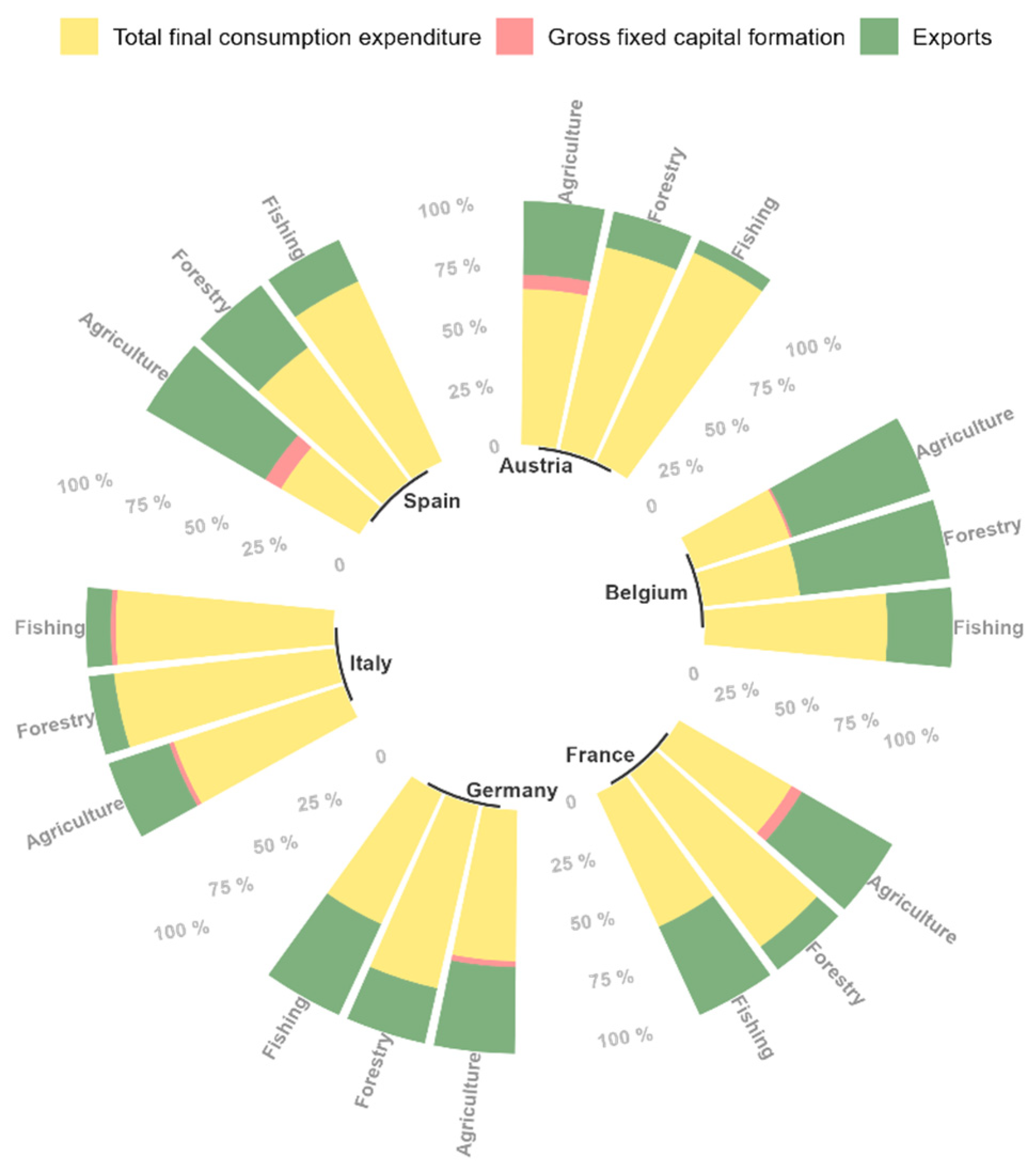
Country	Product	Total Final Consumption Expenditure	Gross Fixed Capital Formation	Exports
Austria	Agriculture	2073.76	191.14	979.25
	Forestry	406.22	0.00	72.41
	Fishing	41.87	0.00	2.57
Belgium	Agriculture	2537.83	63.39	3701.04
	Forestry	93.40	0.00	145.75
	Fishing	167.03	0.00	60.04
France	Agriculture	15,015.05	1374.04	12,086.93
	Forestry	1154.17	0.00	152.98
	Fishing	783.25	0.00	519.02
Germany	Agriculture	17,318.48	674.49	9924.52
	Forestry	1117.48	0.00	337.28
	Fishing	340.93	0.00	237.43
Italy	Agriculture	13,704.94	365.38	4897.40
	Forestry	826.99	0.00	94.03
	Fishing	2066.41	47.70	236.75
Spain	Agriculture	8260.62	1649.21	12,520.33
	Forestry	320.49	0.21	149.85
	Fishing	1942.74	0.00	448.47

presents the same information, but in value terms. The 2010 structure is very similar.

4. Results and Discussion

The proposed decomposition applies to the six EU-28 countries in 2010–2015, for which we have homogeneous information based on symmetric IO tables of total flows, measured in constant prices. In order to perform SDA, price deflation is needed. Here, matrices were deflated considering 2010 prices as base year. Available information about price indexes allows for row and/or columns proportional adjustments (Dietzenbacher and Hoen 1998). These techniques can be adapted to different information scenarios.

Agriculture is the largest of the three selected sectors and is, in fact, the one on which attention is focused. It was decided to present results for the other two similar sectors to test the extended methodology, although calculations were made for all production sectors.

Compared with previous five-year periods, the reference data are characterized by a slowdown, both in final demand and in output by sector. This circumstance is considered ideal for fine-tuning the measurement of technological change using SDA. There has been an upward trend in these macro-economic indicators in the past, so there was no suspicion of possible overestimation in this area.

According to Formula (5), the elements of the main diagonal of the Leontief inverse matrix can be divided into three effects: that produced by final demand, by direct requirement (own consumption), and by indirect requirement. Figure 4 shows this disaggregation for the products examined. This information will be critical for interpreting the normalization results described in the methodology section.

There are no significant differences between the two survey years, but there are some differences among countries. In fact, high values of these multipliers lead to sharp adjustments in the corresponding rows and/or columns, as will be shown in the normalized matrices $—{\tilde{C}}^f$ (row) and ${\tilde{C}}^f$ (col). For example, Forestry’s own consumption in Austria, France and Germany is very high and has its indirect effects, as can be seen in the figure. Moreover, in the case of Belgium and Italy, this sector’s own consumption is zero. Thus, normalization by row and/or column has no effect on the Leontief inverse matrix.

Table 2. Break down of changes in output by country (million EUR) from 2010 to 2015.

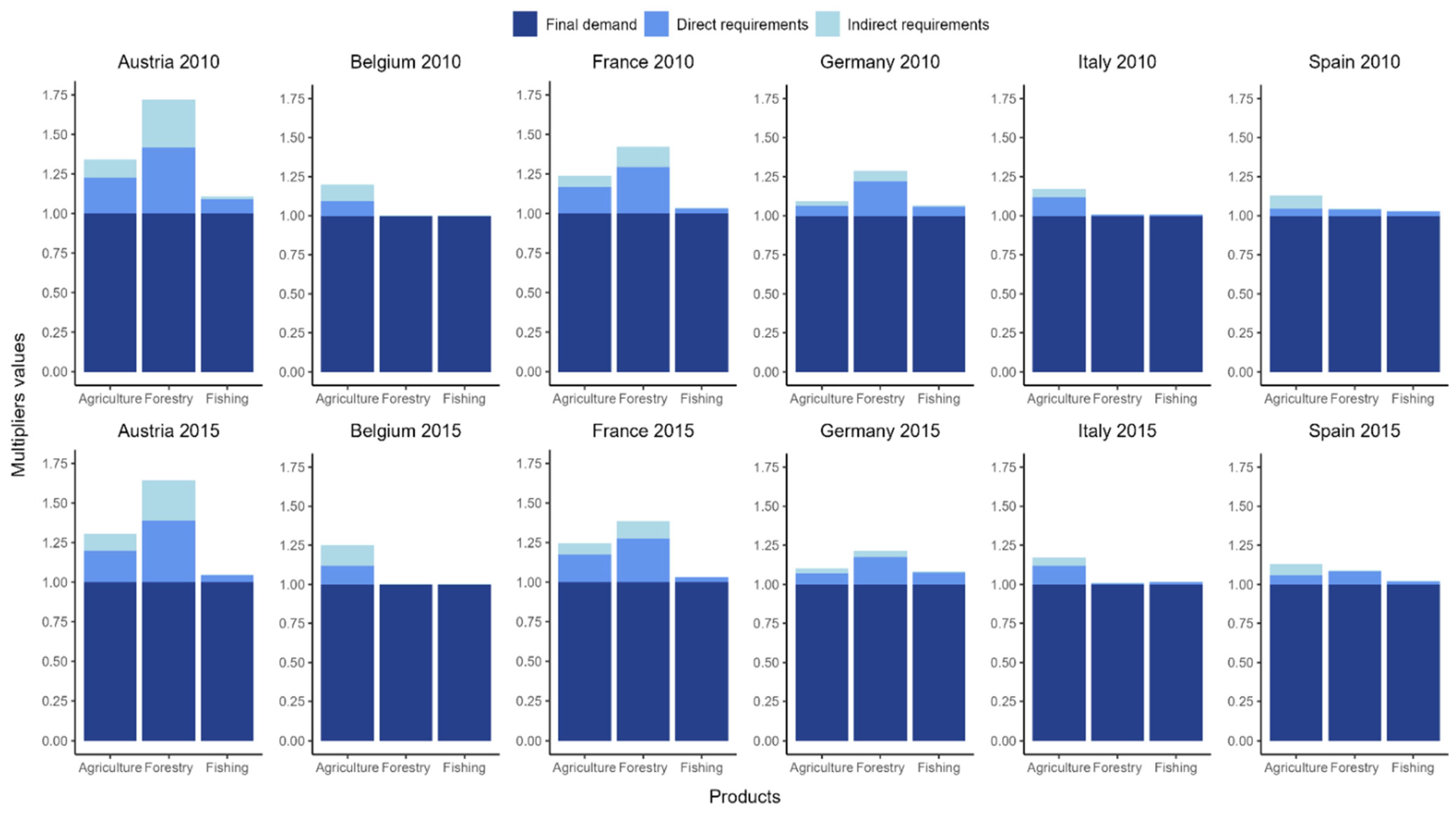
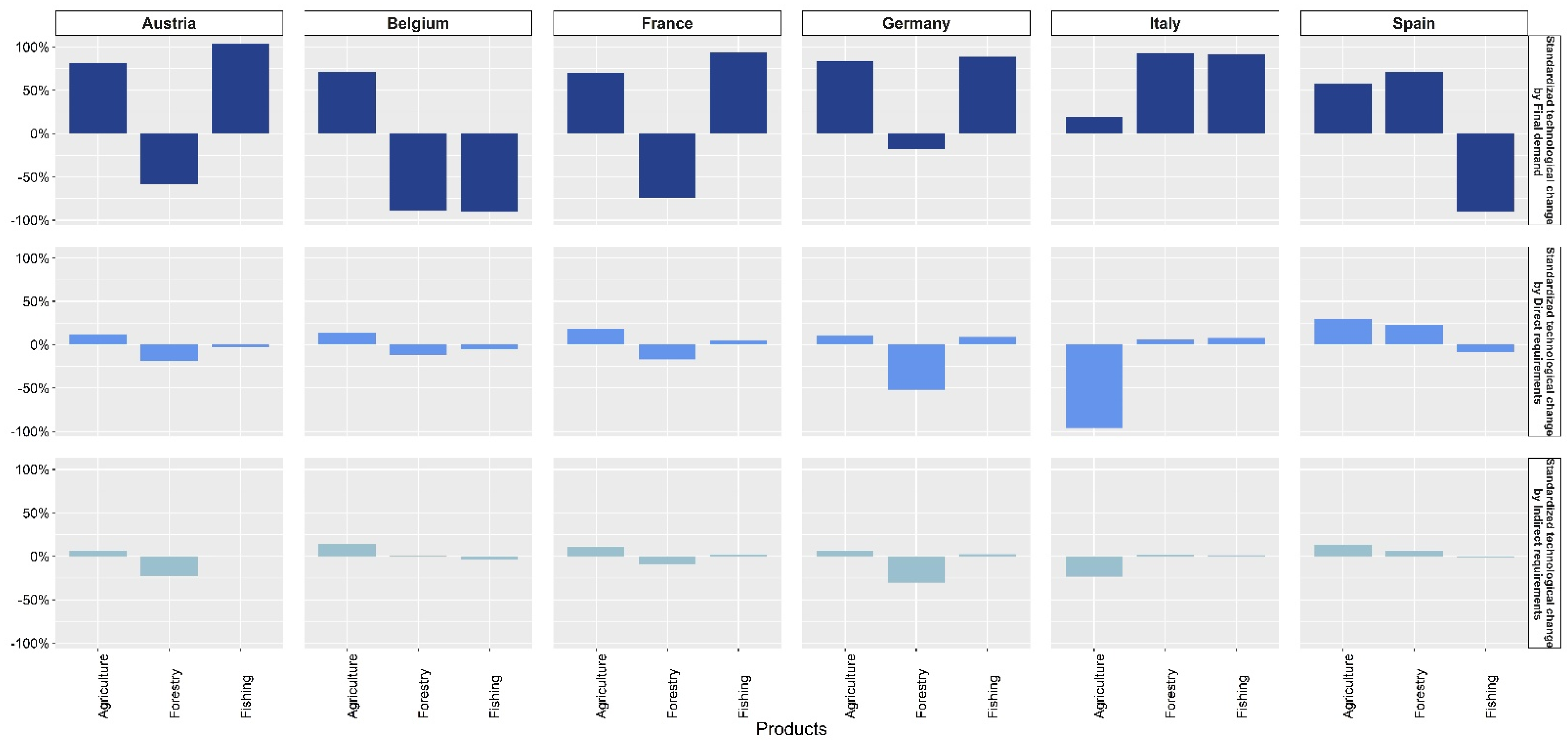
Country	Product	Output Change		Technological Change			Final Demand Change
		Value	%	Standardized by Final Demand	Standardized by Direct Requirements	Standardized by Indirect Requirements	Aggregated
Austria	Agriculture	999.25	18.59	544.45	81.78	44.81	328.21
	Forestry	52.46	2.41	−64.97	−20.66	−25.63	163.71
	Fishing	0.64	1.52	10.52	−0.32	−0.03	−9.53
Belgium	Agriculture	1042.71	12.34	1548.82	310.86	318.44	−1135.41
	Forestry	−6.35	−1.57	−25.13	−3.27	0.07	21.98
	Fishing	−33.23	−25.64	−63.42	−3.96	−2.74	36.88
France	Agriculture	4479.31	7.12	1568.98	418.71	241.55	2250.06
	Forestry	152.84	3.06	−710.22	−163.50	−87.95	1114.52
	Fishing	122.14	5.85	178.06	8.74	4.40	−69.06
Germany	Agriculture	5763.43	14.14	4860.93	599.65	365.42	−62.57
	Forestry	1085.35	34.35	−29.51	−85.93	−49.97	1250.75
	Fishing	44.10	11.67	124.67	12.58	3.44	−96.59
Italy	Agriculture	−1763.27	−3.82	7.15	−35.33	−8.64	−1726.45
	Forestry	89.72	7.06	145.97	8.90	3.37	−68.51
	Fishing	−180.33	−8.33	227.49	19.53	3.14	−430.49
Spain	Agriculture	5512.51	14.00	1755.95	903.09	394.84	2458.64
	Forestry	233.58	19.45	159.77	51.30	14.65	7.86
	Fishing	−345.30	−14.99	−198.02	−18.62	−2.75	−125.91

shows the results for the three primary sectors from 2010 to 2015; although, for computational purposes, all production sectors were considered (see Supplementary Material). The impact of the final demand vector is not broken down. However, it is possible to disaggregate this vector in multiple ways, so it would be possible to apply extended versions of this formula. Additionally, instead of working with an additive format, one can use a multiplicative format. The various disaggregation possibilities shown in Table 2 do not present a common pattern, although they do show some commonalities that are described below. With respect to agriculture, there is an upward trend in production, except for Italy, which can be explained by technological change and final demand changes. However, these recent changes do not always follow the same path. Overall, changes in the other sectors, i.e., forestry and fishing, are not as significant. However, they display different changes to those in agriculture.

The focus is centered on variations due to technological change, which is explained by positive or negative changes in inverses and in the mean vector of final demand, which is always positive. This means that positive or negative changes will be determined by changes in Leontief inverse matrices. In this respect, it should be noted that a reduction in the proportion of intermediate demand results in an increase in the proportion of final demand. Therefore, for the purposes of the inverse, it implies lower values of its components. Over time, this means that negative changes in the inverse imply that there is less dependence on intermediate inputs. In a period, such as the one under consideration, which is characterized by an economic crisis and which at the same time covers only a few years, it can be assumed that almost no changes have taken place in its production structures. Therefore, such a refinement of the overall figures for technological change by roughly subtracting the component attributed to sectoral own consumption could be a suitable alternative for analysis.

The empirical application here presented gives a straightforward probe of how technological changes in SDA analysis, as captured in Miller and Blair (2009), can be disaggregated into different components. A mathematical demonstration has been given in Equations (27)–(32). Since analogous proposals cannot be found in literature to the author´s knowledge, empirical comparisons between alternative decompositions are not possible. However, these methodological improvements could be combined with other SDA developments (e.g., the ones focused on disaggregating final demand components). This could be a promising way forward for further testing.

Figure 5 supports the table of results but focuses only on the decomposition of technological changes. A decomposition of the change indicated by final demand can also be performed, however, that is beyond the scope of this article. The results are shown as percentages to facilitate their visual comparison. Again, heterogeneous behavior is evident. It is clear that the disaggregation of elements of the main diagonal, presented in Figure 4, determines these results because those elements are used as distribution factors. For example, it is clear that agriculture in Italy shows technological improvement, although when we go into detail about it, the change in own consumption determines this global figure and the other two components ultimately offset each other because one is positive and the other negative. Another example to consider is Forestry in Germany, with high own consumption, as stated above, and that the factor attributed to it largely explains the reduction in output in this respect; if this component is deducted, the technological change will not be so marked.

The value of the main diagonal’s components (Leontief inverse matrix) depends largely on own consumption, regardless of the interrelationships that each production sector has with the others that make up the economy. Even mere errors in the calculation of own consumption may be considered to be technological changes when they are not. In this sense, agricultural products are very diverse but in the formatting processes of symmetric IO tables they are presented grouped together. Moreover, the symmetric format almost always needs to be adjusted by algorithms that can often raise figures of a higher value. In future research, the output changes could be analyzed using rectangular IO models because origin–destination tables present a greater disaggregation of basic products and do not depend on purely mathematical adjustments that ensure accounting equilibrium, but which may, in some way, distort true relationships between product demand and output by non-homogeneous branches of production.

5. Conclusions

Primary sectors are ideal for testing the extended SDA, since they are closely interconnected with the rest of the economy, and at the same time, they tend to have higher than average own consumption figures. With respect to the Leontief model, the own consumption figures treated through normalization do not change the accounting balance, hence it is possible to make transformations to the above-mentioned model, which facilitate the calculation of net effects. Furthermore, the presented normalizations of the Leontief inverse matrix and its decomposition facilitate the calculation of the importance of a sector in terms of its external contribution—associated with sectoral interdependencies—and also reproduce the size of the corresponding economy. In terms of comparing the accounting frameworks, whether for the economy as a whole or for the production sector, the sectoral own consumption can also be relativized. In this way, at least in part, the effect they have on the calculation of multipliers to compare inverses from different years can be deduced. The sensitiveness of inverse elements can be fine-tuned, or other means can be employed to adjust or refine concepts such as technological change. Within IO frameworks, this kind of normalizations have also been used to measure inter-industrial linkages (Pereira-López et al. 2021).

In the processes of constructing homogeneous branches (a product equals a branch) in equilibrium, some adjustments are applied that tend to raise the figures of a higher value, and own consumption figures are an excellent candidate for such an accumulation of errors (adjustments). Hence, the output changes could be analyzed using rectangular IO models because they operate with a greater disaggregation of basic products, and they are not subject to accounting adjustments.

References

- Avelino, Andre F. T., and Sandy Dall’erba. 2020. What factors drive the changes in water withdrawals in the U.S. Agriculture and food manufacturing industries between 1995 and 2010? Environmental Science and Technology 54: 10421–34. [Google Scholar] [CrossRef]
- Cai, Beiming, Wei Zhang, Klaus Hubacek, Kuishuang Feng, Zhenliang Li, Yawen Liu, and Yu Liu. 2019. Drivers of virtual water flows on regional water scarcity in China. Journal of Cleaner Production 207: 1112–22. [Google Scholar] [CrossRef]
- Casler, Stephen D., and Adam Rose. 1998. Carbon dioxide emissions in the U.S. economy: A structural decomposition analysis. Environmental and Resource Economics 11: 349–63. [Google Scholar] [CrossRef]
- Cellura, Maurizio, Sonia Longo, and Marina Mistretta. 2012. Application of the Structural Decomposition Analysis to assess the indirect energy consumption and air emission changes related to Italian households consumption. Renewable and Sustainable Energy Reviews 16: 1135–45. [Google Scholar] [CrossRef]
- Chen, Chia Yon, and Rong Hwa Wu. 1994. Sources of change in industrial electricity use in the Taiwan economy, 1976–1986. Energy Economics 16: 115–20. [Google Scholar] [CrossRef]
- Chen, Yen Yin, and Jung Hua Wu. 2008. Simple Keynesian input–output structural decomposition analysis using weighted Shapley value resolution. Annals of Regional Science 42: 879–92. [Google Scholar] [CrossRef]
- Dietzenbacher, Erik, and Alex R. Hoen. 1998. Deflation of input–output tables from the user’s point of view: A heuristic approach. Review of Income and Wealth 44: 111–22. [Google Scholar] [CrossRef]
- Dietzenbacher, Erick, and Bart Los. 1998. Structural decomposition techniques: Sense and sensitivity. Economic Systems Research 10: 307–24. [Google Scholar] [CrossRef]
- Doan, Ha Thi Thanh, and Trinh Quang Long. 2019. Technical change, exports, and employment growth in china: A structural decomposition analysis. Asian Economic Papers 18: 29–46. [Google Scholar] [CrossRef]
- Eurostat. 2015a. ESA Supply, Use and Input–output Tables-Eurostat. Available online: https://ec.europa.eu/eurostat/web/esa-supply-use-input-tables/data/database (accessed on 25 March 2020).
- Eurostat. 2015b. Eurostat-Data Explorer. Available online: https://appsso.eurostat.ec.europa.eu/nui/show.do?dataset=nama_10_a64&lang=en (accessed on 25 March 2020).
- Fang, Dan, and Jin Yang. 2021. Drivers and critical supply chain paths of black carbon emission: A structural path decomposition. Journal of Environmental Management 278: 111514. [Google Scholar] [CrossRef]
- Feng, Le, Bin Chen, Tasawar Hayat, Ahmed Alsaedi, and Bashir Ahmad. 2017. The driving force of water footprint under the rapid urbanization process: A structural decomposition analysis for Zhangye city in China. Journal of Cleaner Production 163: S322–S328. [Google Scholar] [CrossRef]
- Forssell, Osmo. 1990. The input–output framework for analysing changes in the use of labour by education levels. Economic Systems Research 2: 363–76. [Google Scholar] [CrossRef]
- Fujimagari, David. 1989. The sources of change in canadian industry output. Economic Systems Research 1: 187–202. [Google Scholar] [CrossRef]
- Gerveni, Maria, Andre F. T. Avelino, and Sandy Dall’erba. 2020. Drivers of Water Use in the Agricultural Sector of the European Union 27. Environmental Science and Technology 54: 9191–99. [Google Scholar] [CrossRef] [PubMed]
- Gim, Ho Un, and Koonchan Kim. 1998. The general relation between two different notions of direct and indirect input requirements. Journal of Macroeconomics 20: 199–208. [Google Scholar] [CrossRef]
- Gim, Ho Un, and Koonchan Kim. 2005. The decomposition by factors in direct and indirect requirements: With applications to estimating the pollution generation. The Korean Economic Review 21: 309–25. [Google Scholar]
- Han, Xiaoli, and T. K. Lakshmanan. 1994. Structural changes and energy consumption in the Japanese economy 1975–85: An input–output analysis. Energy Journal 15: 165–88. [Google Scholar] [CrossRef]
- Han, Xiaoli. 1995. Structural change and labor requirement of the Japanese economy. Economic Systems Research 7: 47–66. [Google Scholar] [CrossRef]
- Hoekstra, Rutger, and Jeroen. C. J. M. Van Der Bergh. 2003. Comparing structural and index decomposition analysis. Energy Economics 25: 39–64. [Google Scholar] [CrossRef]
- Jacobsen, Henrik K. 2000. Energy demand, structural change and trade: A decomposition analysis of the Danish manufacturing industry. Economic Systems Research 12: 319–43. [Google Scholar] [CrossRef]
- Jeong, Ki Jun. 1982. Direct and indirect requirements: A correct economic interpretation of the Hawkins-Simon conditions. Journal of Macroeconomics 4: 349–56. [Google Scholar] [CrossRef]
- Jeong, Ki Jun. 1984. The relation between two different notions of direct and indirect input requirements. Journal of Macroeconomics 6: 473–76. [Google Scholar] [CrossRef]
- Li, Dongrui, Yalin Lei, Li Li, and Lingna Liu. 2020. Study on industrial selection of counterpart cooperation between Jilin province and Zhejiang province in China from the perspective of low carbon. Environmental Science and Pollution Research 27: 16668–76. [Google Scholar] [CrossRef]
- Li, Wei, Yuyan Huang, and Can Lu. 2020. Exploring the driving force and mitigation contribution rate diversity considering new normal pattern as divisions for carbon emissions in Hebei province. Journal of Cleaner Production 243: 118559. [Google Scholar] [CrossRef]
- Li, Xin, Xiaoqiong He, Xiyu Luo, Xiandan Cui, and Minxi Wang. 2020. Exploring the characteristics and drivers of indirect energy consumption of urban and rural households from a sectoral perspective. Greenhouse Gases: Science and Technology 10: 907–24. [Google Scholar] [CrossRef]
- Liu, Dunnan, Xiaodan Guo, and Bowen Xiao. 2019. What causes growth of global greenhouse gas emissions? Evidence from 40 countries. Science of the Total Environment 661: 750–66. [Google Scholar] [CrossRef] [PubMed]
- Liu, Li-Jing, and Qiao-Mei Liang. 2017. Changes to pollutants and carbon emission multipliers in China 2007–2012: An input–output structural decomposition analysis. Journal of Environmental Management 203: 76–86. [Google Scholar] [CrossRef] [PubMed]
- Miller, Ronald E., and Peter D. Blair. 2009. Input–output Analysis: Fundations and Extensions, 2nd ed. Cambridge: Cambridge University Press. [Google Scholar]
- Mukhopadhyay, Kakali, and Debesh Chakraborty. 1999. India’s energy consumption changes during 1973/74 to 1991/92. Economic Systems Research 11: 423–38. [Google Scholar] [CrossRef]
- Muradov, Kirill. 2021. Structural decomposition analysis with disaggregate factors within the Leontief inverse. Journal of Economic Structures 10: 1–17. [Google Scholar] [CrossRef]
- Pereira-López, Xesús, Małgorzata Anna Węgrzyńska, and Melchor Fernández-Fernández. 2021. Methodological contribution to the detection of backward linkages between sectors of the economy. Argumenta Oeconomica 46: 31–52. [Google Scholar] [CrossRef]
- Qian, Yiying, Huijuan Dong, Yong Geng, Shaozhuo Zhong, Xu Tian, Yanhong Yu, Yihui Chen, and Dana Avery Moss. 2018. Water footprint characteristic of less developed water-rich regions: Case of Yunnan, China. Water Research 141: 208–16. [Google Scholar] [CrossRef]
- Rose, Adams, and Chia-Yon Chen. 1991. Sources of change in energy use in the US economy, 1972–1982: A structural decomposition analysis. Resources and Energy 13: 1–21. [Google Scholar] [CrossRef]
- Rose, Adams, and Stephen Casler. 1996. Input–output structural decomposition analysis: A critical appraisal. Economic Systems Research 8: 33–62. [Google Scholar] [CrossRef]
- Song, Yi, Jianbai Huang, Yijun Zhang, and Zhiping Wang. 2019. Drivers of metal consumption in China: An input–output structural decomposition analysis. Resources Policy 63: 101421. [Google Scholar] [CrossRef]
- Sonis, Michael, Geoffrey J. Hewings, and Jiemin Guo. 1996. Sources of structural change in input–output systems: A field of influence approach. Economic Systems Research 8: 15–32. [Google Scholar] [CrossRef]
- Supasa, Tharinya, Shu-San Hsiau, Shih-Mo Lin, Wongkot Wongsapai, and Jiunn-Chi Wu. 2017. Household energy consumption behaviour for different demographic regions in Thailand from 2000 to 2010. Sustainability 9: 2328. [Google Scholar] [CrossRef] [Green Version]
- Wang, Fei, Baomin Dong, Xiaopeng Yin, and Chi An. 2014. China’s structural change: A new SDA model. Economic Modelling 43: 256–66. [Google Scholar] [CrossRef]
- Wang, Xiaomeng, Kai Huang, Yajuan Yu, Tingting Hu, and Yanjie Xu. 2016. An input–output structural decomposition analysis of changes in sectoral water footprint in China. Ecological Indicators 69: 26–34. [Google Scholar] [CrossRef]
- Wood, Richard, and Manfred Lenzen. 2009. Structural path decomposition. Energy Economics 31: 335–41. [Google Scholar] [CrossRef]
- Xu, Shichun, Wenwen Zhang, Qinbin Li, Bin Zhao, Shuxiao Wang, and Ruyin Long. 2017. Decomposition analysis of the factors that influence energy related air pollutant emission changes in China using the SDA method. Sustainability 9: 1742. [Google Scholar] [CrossRef] [Green Version]
- Yu, Yang, Tangyang Jiang, Shuangqi Li, Xiaolong Li, and Dingchao Gao. 2020. Energy-related CO2 emissions and structural emissions’ reduction in China’s agriculture: An input–output perspective. Journal of Cleaner Production 276: 124169. [Google Scholar] [CrossRef]
- Zhi, Yuan, Z. F. Yang, and X. A. Yin. 2014. Decomposition analysis of water footprint changes in a water-limited river basin: A case study of the Haihe River basin, China. Hydrology and Earth System Sciences 18: 1549–59. [Google Scholar] [CrossRef] [Green Version]