Public Debt and Economic Growth in EU Countries

Abstract

The short- and long-term effects of public debt on economic growth in EU countries is analyzed in this paper, using data that covers a period of 25 years (1995–2019). For public debt, we used a proxy general government gross debt (as a percentage of GDP), while for economic growth, we used the real GDP per capita growth rate. In addition, our models include a set of control variables to highlight the impact of other determinants on economic growth. We utilized several econometric methodologies related to ARDL (autoregressive distributed lag models), such as the pooled mean group (PMG), the mean group (MG), and the dynamic fixed effects (DFE) models. The results of the study show that in both the short and long term, an increase in public debt is negatively and significantly associated with economic growth. Specifically, in both the short- and long-term analyses, the estimated coefficients of public debt were statistically significant and negative, while the magnitude of the negative impact on economic growth differed. In view of these findings, we consider both the rigorous monitoring of the level of public debt and the control of public allocation to support economic growth to be of major importance.

1. Introduction

The link between public debt (control) and economic growth is one of the macro-economic issues that has been intensely debated by economists due to its economic and social implications, as well as its complexity.

Economic theory maintains that public debt can either stimulate the economy or hinder economic growth depending on the size and structure of the public debt, but also on the allocation of the borrowed resources. The positive effects of public debt would manifest only if the borrowed funds were used to finance productive government expenditures, which would promote solid and sustainable economic growth. According to the conventional view, public debt has a positive effect on short-term economic growth by stimulating demand and production. However, economic theory indicates that, in the long run, an increase in public debt has a negative impact on growth by crowding-out private investment. High public debt can discourage private investment and curb economic growth through higher long-term interest rates, higher inflation, higher future distortionary taxation, and greater uncertainty about prospects and policies (Kumar and Woo 2010).

The unprecedented increase in public debt in all the countries of the world, including the member states of the European Union, but especially those in the euro area, amid the recent international crisis has led to a considerable increase in the interest of researchers and policymakers in examining the economic impact of increasing public debt. Starting with two fundamental papers by Reinhart and Rogoff (2010a, 2010b) on the impact of public debt on economic growth, a growing number of studies have empirically explored the relationship between public debt and economic growth and have sought to identify the level from which debt starts to have a detrimental effect on economic growth. However, the research results in the literature are ambiguous due to the time period analyzed, the sample of countries considered, and the empirical methodology used. Moreover, there is no clear evidence of a causal relationship between public debt and economic growth (Panizza and Presbitero 2014) by which an increased level of the public debt-to-GDP ratio would lead to decreased economic growth, or, vice versa, by which weak economic growth would lead to an increased public debt.

The current economic crisis generated by the COVID-19 pandemic has led to significantly increased public debt and reduced economic activity in many states, including those that are part of the EU (Butkus et al. 2021). This has deepened the concern regarding the possible adverse effects of the accumulation of public debts. In this context, the rise in academic debates and in policy makers’ discussions regarding the nexus between public debt and economic growth is of interest, especially in terms of the possible impact of increased public debt on economic growth.

Given the so far unclear correlation between the level of public debt and economic growth and given the need to establish whether public debt hinders or stimulates eco-nomic growth, the main objective of our study is to empirically examine the long- and short-term impact of public debt on economic growth in EU countries using data covering the period 1995–2019. We utilize several econometric methodologies related to ARDL (autoregressive distributed lag models), such as the pooled mean group (PMG), the mean group (MG), and the dynamic fixed effects (DFE) models, using the methodology proposed by Blackburne and Frank in 2007, as well as the method proposed by (Chudik and Pesaran 2013, 2015) and implemented by Ditzen (2018), which controls for common-correlated effects. The use of the ARDL is based on dependence of the dependent variable on its own lags. The choice is better explained in the literature review and in Section 4. The proposed methodology (error-correction model) is based on controlling at least for: non-stationary in levels for the series, cointegration between variables, the presence of some outliers, the long-run relations on variables implied. Further explanations are available in Section 4, Results and Discussion.

The previous research on public debt and economic growth shows that most studies have analyzed the impact of public debt on economic growth, either in the short or long term, but few studies have considered both time periods.

The added value of the study lies in a more up-to-date analysis and the use of new empirical methodologies.

This paper contributes to the literature that is focused on the link between public debt and economic growth in two ways. First, we offer new insights into the short- and long-term effects of public debt on economic growth in 28 European countries (including the UK) using the latest data available for the analyzed variables. Secondly, our research uses new empirical models based on the research methodology of Chudik and Pesaran (2013, 2015), as mentioned above. To our knowledge, there are few studies, especially few recent ones, that have evaluated the short- and long-term effect of public debt on economic growth using the ARDL approach considering all the EU countries. Therefore, our research fills this gap, providing new empirical evidence regarding the possible impact of public debt on economic growth in 28 EU countries, in both the short and long term.

The remainder of this study is organized as follows: Section 2 briefly reviews the literature, especially the empirical findings on public debt and economic growth. Section 3 explains the data and presents the empirical methodology. Section 4 reports the empirical results and the related discussion. Finally, Section 5 offers some concluding remarks.

2. Literature Review

A topic of interest discussed in several studies focused on examining the relationship between public debt and economic growth refers to the channels through which public debt could affect economic growth. Knowing them is important for policymakers in order to adopt measures that allow the control of public debt and the stimulation of economic growth. Pattillo et al. (2004) empirically argues that a high level of debt would have a negative impact on economic growth through the strong negative effect on capital accumulation and productivity growth. Other authors (Sutherland and Hoeller 2012) point out that a high level of debt can negatively affect macroeconomic performance by reducing the possibility for a government to react effectively to adverse shocks. Another key channel is that of interest rates through which public debt would influence financial stability, private spending and, therefore, economic growth (Časni et al. 2014). In the study developed by Checherita-Westphal and Rother (2012), attention is focused on the empirical examination of the impact of public debt on economic growth in the euro area through several channels, namely private saving and private investment rate, public investment rate, total factor productivity, and sovereign long-term nominal and real interest rates. The authors find that public debt can have a non-linear effect on economic growth through the channels of private saving, public investment and total factor productivity.

The analysis of the literature on public debt and economic growth reveals the existence of an impressive number of studies, both theoretical and empirical, that have examined the relationship between public debt and economic growth. However, there is no solid evidence to confirm a definitive negative or positive relationship between public debt and GDP growth. In a systematic review of 33 articles, Rahman et al. (2019) highlighted that such a relationship can be negative, positive, or even non-linear. An increasing number of empirical studies have indicated an inverted U-shape relationship between public debt and growth; therefore, the impact of low-level public debt on economic growth is positive, while beyond a certain threshold, public debt has a negative effect on economic growth (Kumar and Woo 2010; Reinhart and Rogoff 2010a, 2010b; Checherita-Westphal and Rother 2012; Baum et al. 2013; Mencinger et al. 2014, 2015; Bilan and Ihnatov 2015; Law et al. 2021; Liu and Lyu 2021). Kumar and Woo (2010) identified an inverse relationship between initial debt and subsequent growth for a sample of developed and emerging countries in the period 1970–2007. Their research results showed that, when the debt-to-GDP ratio increased by ten percentage points, the annual growth of real GDP per capita decreased by about 0.2 percentage points per year, with a smaller effect in the case of developed countries. Their research also indicated that only high levels of debt (above 90 percent of GDP) have a significant effect on economic growth. In this regard, Reinhart and Rogoff (2010a), using data covering the period 1790–2009 and focusing on a sample of 44 developed and emerging countries found that when debt was below 90% of GDP, its effect on economic growth was positive but weak, while the effect was negative and significant when the debt was above the threshold of 90% of GDP. The results of the study by Reinhart and Rogoff (2010a) regarding the impact of government debt on economic growth have given rise to a series of disputes and have led to an intensification of the concerns of some authors to assess to what extent the findings of Reinhart and Rogoff (2010a) would be solid. Thus, Herndon et al. (2013) empirically analyze the results of Reinhart and Rogoff (2010a, 2010b) and find that the relationship between public debt and economic growth would be incorrect due to some coding errors, the exclusion of some available data and an unconventional weighting of summary statistics. The authors also argue that the relationship between public debt and economic growth varies significantly, depending on the time period analyzed and the country. In addition, some authors (such as Panizza and Presbitero 2013; Eberhardt and Presbitero 2015) show that there is no evidence of a common debt threshold beyond which economic growth would decrease significantly. In another study, Panizza and Presbitero (2014) argue that the link between public debt and growth disappears once endogeneity is corrected.

Several studies (presented below) have empirically argued that the relationship between public debt and economic growth is non-linear. In addition, the authors of the mentioned studies emphasize that this relationship is characterized by great heterogeneity between countries and may vary over time within countries.

The study by Checherita-Westphal and Rother (2012) analyzed the impact of public debt on economic growth for 12 eurozone member states for the period 1970–2010. The results of the study indicated a highly statistically significant non-linear relationship between public debt and the GDP per capita growth rate. The authors found that the effects of public debt on economic growth were negative when public debt reached a level of about 90–100% of GDP. Referring to the same twelve countries in the euro area but analyzing a different time period and using a different research methodology, Baum et al. (2013) found that public debt lower than 67% of GDP had a positive impact on short-term economic growth; however, the effects became insignificant beyond this threshold, and were negative when the debt ratios increased to over 95% of GDP. The study conducted by Mencinger et al. (2014) analyzed the short-term impact of public debt on economic growth, taking into account a sample of 25 EU member states for the period 1980–2010. Their empirical results indicated a non-linear and concave relationship between public debt and economic growth. In addition, the authors calculated the threshold value of public debt, which was approximately between 80% and 94% for the “old” member states and between 53% and 54% for the “new” member states. Using a panel dataset for 31 OECD member states and 5 non-OECD EU member countries, Mencinger et al. (2015) examined the effects of public debt on economic growth in the short term. The results showed that the impact of low-level public debt on economic growth was positive, while beyond a certain turning point, debt had a negative effect. The authors also determined the public debt-to-GDP turning point, which was between 90% and 94% for developed economies and between 44% and 45% for emerging countries. Using data for 118 countries, Eberhardt and Presbitero (2015) found a negative long-run relationship between a country’s public debt and growth. In addition, the authors stressed that the link between public debt and economic growth is complex and, in order to identify the tipping point beyond which an increase in public debt has detrimental effects on economic growth, the characteristics of each country must be taken into account. Égert (2015) in his paper supported the existence of a negative non-linear relationship between public debt and economic growth but emphasized that such a relationship would greatly depend on the time period and the countries analyzed, as well as the empirical models used. The author showed that, when a non-linear relationship is identified, levels of public debt between 20% and 60% of GDP already exert negative effects on growth.

The relationship between public debt and economic growth was also empirically explored by Chudik et al. (2017) based on a dataset for 19 developed countries and 21 developing countries for the period 1965–2010. The authors investigated the value of the public debt threshold beyond which economic growth falls significantly. Their study identified a debt threshold of between 60% and 80% for the entire sample of countries, of 80% for the developed countries, and between 30% and 60% for the developing countries. In addition, the study showed that, regardless of the debt threshold, there was a negative and significant relationship between increasing public debt and economic growth in the long run.

A more recent study (Fetai et al. 2020) examined the extent to which public debt growth affected economic growth in the European transition countries for the period 1995–2017. The results of the study showed a non-linear and concave relationship between public debt and economic growth, as well as the fact that the threshold values of public debt differed among European transition countries. The authors found that the threshold value of the debt-to-GDP ratio was lower for less developed European transition countries than that of developed European transition countries.

Identifying the critical point or threshold of the public debt-to-GDP ratio is of great interest to researchers and policymakers because it is a crucial element in the design of a fiscal policy aimed at avoiding excessive indebtedness (Law et al. 2021). Bentour (2021) emphasized that there is no public debt threshold common to all the countries and that the relationship between public debt and economic growth varies either at country level, sample level, or depending on the time period analyzed. Moreover, Pescatori et al. (2014) sustained that there is no clear evidence that economic growth is bound to suddenly deteriorate beyond a certain threshold of debt to GDP. Analyzing the cases of the countries with a substantial debt that showed a decreasing trend, the authors showed that these countries’ economic growth registered similar increasing performances to those of the less indebted countries. These results sustain the idea that the trajectory of debt is a more important predictor of future economic growth than the level of debt.

The research paper by Liu and Lyu (2021) revealed that there is a non-linear relationship between public debt and economic growth, both in developing and emerging countries, and in developed countries. However, the debt threshold differs from one country to another, depending mainly on the current account balance, gross savings, crisis, and the degree to which the economy is opened. Comparatively, other studies—such as (Bilan and Ihnatov 2015; Eberhardt and Presbitero 2015; Ramos-Herrera and Sosvilla-Rivero 2017)—have highlighted the presence of a heterogeneity in the relationship between debt and growth, in the sense that the effects of public debt on growth may vary depending on the macroeconomic, financial, and institutional variables specific to each country. Analyzing the recent literature on the link between public debt and economic growth, Panizza and Presbitero (2013) pointed out that the relationship between these two variables is characterized by a large cross-country heterogeneity and may vary within countries over time. Similarly, Chudik et al. (2017) showed that the impact of public debt on economic growth differs from country to country depending on country-specific factors, such as the degree of their financial deepening, the history of past debt settlement, and the nature of their political system. Using a panel dataset for 82 countries, Kourtellos et al. (2013) argued that the effect of public debt on growth depends on a country’s democratic institutions. The results of the study indicated that, in countries with poor institutional quality, the impact of public debt on economic growth was negative, while in countries with a high-quality institutional framework, the impact of public debt was neutral. Using data for EU countries, Masuch and Moshammer (2017) argued that the significant negative effect of high-level public debt on long-term economic growth could be mitigated by the presence of well-established institutions. Among recent studies, Law et al. (2021) noted for a panel of developing countries, that high levels of public debt are detrimental to economic growth; however, such negative effects could be minimized by the presence of high-quality institutions.

Several studies—e.g., (Gómez-Puig and Sosvilla-Rivero 2018; Časni et al. 2014; Afonso and Alves 2015; Albu and Albu 2021; Asteriou et al. 2021)—have focused on examining the link between public debt and economic growth, both in the short and long term, using different econometric models. Thus, based on a dataset for a sample of 14 central, eastern, and south-eastern European countries for the period 2000–2011, Časni et al. (2014) demonstrated that public debt has a significant negative effect on GDP growth, both in the short and long term. The authors emphasized the need to design policy frameworks that encourage exports and promote long-term investment so as to stimulate sustainable growth. The results of the study were confirmed by the paper by Afonso and Alves (2015), which analyzed 14 European countries for a period of 43 years (1970–2012). They found that debt service had a greater negative effect on economic growth than public debt. Using data for 20 developing countries, Lof and Malinen (2014) did not find a statistically significant effect of debt on economic growth in the long term. Moreover, in their study they highlighted that in the long term, the negative correlation between public debt and GDP growth mainly refers to the negative influence of economic growth on public debt. Similarly, but referring to 26 developing countries, Vanlaer et al. (2015) found that in the short term, an increased level of public debt has a negative effect on economic growth, while the impact is weaker in the medium term and non-existent in the long term. The authors sustained that weak economic growth leads to an increased level of debt, but not the other way around. Jacobs et al. (2020) empirically explored the relationship between public debt and economic growth for 31 EU and OECD countries. The authors did not find a causal relationship between public debt and economic growth, regardless of the level of public debt. Instead, they found a causality between economic growth and public debt, which suggests that weak economic growth leads to an increase in the level of public debt by increasing the real interest rate in the long term. In comparison, Gómez-Puig and Sosvilla-Rivero (2017) empirically explored the link between public debt and economic growth by using the ARDL (autoregressive distributed lag) method for a database of 11 Eurozone countries for the period 1961–2013. The results of the study showed that public debt always exerts a negative impact on long-term economic growth, while its short-term effects could be positive, depending on the country. The authors argued that high public debt hinders economic growth by increasing uncertainty over future taxation, crowding out private investment, and weakening a country’s resilience to shocks.

When analyzing the literature, we found a small number of papers, especially recent ones, that examined the impact of public debt on economic growth in all of the European Union countries. In addition, we found that few papers have used the ARDL approach and assessed both the short- and long-term effects of public debt on economic growth. Thus, this paper complements the literature by empirically estimating the short- and long-term effects of public debt on economic growth in 28 European countries, using the ARDL approach.

3. Data, Variables, and Methodology

The aim of our research was to identify and analyze the short- and long-term effects of public debt on economic growth. Our analysis focuses on the 28 EU member states (the United Kingdom was taken into account because, at the time of the analysis, it was part of the EU) and covers a period of 25 years (1995–2019).

The dependent variable in our models is represented by the real GDP per capita growth rate, used as a proxy for economic growth. The key explanatory variable is public debt, measured in our study by the general government gross debt as a percentage of GDP. In addition, our models include a set of control variables to highlight the impact of other determinants of economic growth. These variables were selected according to other empirical studies—such as (Kumar and Woo 2010; Bilan and Ihnatov 2015; Mencinger et al. 2015; Afonso and Alves 2015; Gómez-Puig and Sosvilla-Rivero 2017)—and are represented by gross fixed capital formation (gfc), the general government total expenditure (exp), the openness of the economy (open), the inflation rate (infl), the population growth rate (popgr), and the general government budget balance (ggbb).

The data on these variables were mainly obtained from the IMF’s World Economic Outlook Database and Historical Public Debt Database, and the World Bank’s World Development Indicators (WDI) Database. A brief description of the variables and data sources is highlighted in

Table 1. Description of the variables and data sources.

Variable Name (Symbol)	Definition	Data Source
Real GDP per capita growth rate (rgdp)	Annual percentage growth rate of GDP per capita based on constant local currency.	World Bank (World Development Indicators)
Public debt (debt)	General government gross debt (% of GDP).	International Monetary Fund (Historical Public Debt Database); IMF Country Report, 1999, for Bulgaria (1995–1996); AMECO for Latvia, Lithuania (1995–1997), and Romania (1995–1999)
GDP per capita (gdp)	GDP per capita (constant 2010 USD).	World Bank (World Development Indicators)
Gross fixed capital formation (% of GDP) (gfc)	Gross capital formation focuses on physical investments, such as land improvements, buying equipment or machinery, etc.	World Bank (World Development Indicators)
General government total expenditure (% of GDP) (exp)	Total expenditure consists of total expenses and the net acquisition of nonfinancial assets.	International Monetary Fund (World Economic Outlook Database); AMECO for Bulgaria (1995–1997), Estonia (1995–1997), and Malta (1995–1999)
Openness of the economy (% of GDP) (open)	The sum of exports and imports of goods and services as % GDP.	World Bank (World Development Indicators)
Inflation rate (annual %) (infl)	The annual percentage change in the cost of acquiring a basket of goods and services.	World Bank (World Development Indicators)
Population growth (annual %) (popgr)	Annual population growth rate of the population from year t-1 to t, expressed as a percentage.	World Bank (World Development Indicators)
General government budget balance (% of GDP) (ggbb)	General government net lending/borrowing (percent of GDP).	International Monetary Fund (World Economic Outlook Database); AMECO for Bulgaria (1995–1997), Latvia (1995–1997), and Malta (1995–1999)

Source: authors’ own elaboration.

.

The econometric methodology is generally based on a pooled OLS general model that does not account for distinct entities and refers to the classical linear regression, as described in equation no. (1). Here, we explain the general model and time series model; finally, we focus on panel data, accounting for differences in individual means related to country specifics.

$${\mathit{Y}}_t={\mathit{\beta }}_1+{\mathit{\beta }}_2{X}_t+{\mathit{\mu }}_t$$

(1)

The main disadvantage of the classical linear regression model is that it requires X and Y to be stationary in covariance. A major problem that could be encountered is the presence of non-stationarity in the data that can be verified, for instance, with the Dickey and Fuller test (DF test; Dickey and Fuller 1979), which checks for the existence of a unit root, based on the AR(1) model. Sometimes, the error term may not be white noise; in this situation, an augmented version of the test (ADF test) that includes additional lagged terms of the dependent variable in order to control for serial correlation in the test equation, is used. Further, using the method of moments for standard errors to account for serial correlation—as in Newey and West (1987)—Phillips and Perron (1988) developed a generalization of the ADF test procedure. The choice of methodology is related to the fact that in time series and panel data, the variables are usually co-integrated, making it necessary to rely on an error-correction model (ECM), which is stationary.

To test the stationarity in the panels, we used a variety of tests (for unit roots) in the panel dataset. Tests (Levin et al. 2002; Harris and Tzavalis 1999; Breitung and Das 2005; Im et al. 2003) and the Fisher-type (Choi 2001) have the null hypothesis H0: all the panels contain a unit root. The LM test (Hadri 2000) has the null hypothesis H0: all the panels are (trend) stationary.

We present, in Equation (2), the autoregressive distributed lag models ARDL (p, q) as a theoretical base for the ECM model (3).

In autoregressive distributive lag models, when variables are co-integrated in (4), the error term is an I(0) process for all i (units). The model estimates the responsiveness to any deviation from a long-run equilibrium; therefore, in the error-correction model, the short-run dynamics of the variables (in the system) may be influenced by their deviation from the equilibrium. The model from (2) refers to the estimation of non-stationary heterogeneous panels (Blackburne and Frank 2007).

$$y_{it}={\displaystyle \sum }_{j=1}^p{\lambda }_{ij}{y}_{i,t-j}+{\displaystyle \sum }_{j=0}^q{\delta }_{ij}^{\prime }{X}_{i,t-j}+{\mu }_i+{ϵ}_{it},$$

(2)

In the case of non-stationary variables and cointegration, an error-correction term is used, so the model can be written as Equation (3).

$$\begin{array}{l}\mathsf{\Delta }{y}_{it}={\varphi }_i\left(y_{i,t-1}-{\theta }_i^{\prime }{X}_{it}\right)+{\displaystyle {\displaystyle \sum }_{j=1}^{p-1}}{\lambda }_{ij}^{*}n\mathsf{\Delta }{y}_{i,t-1}+{\displaystyle {\displaystyle \sum }_{j=0}^{q-1}}{\delta }_{ij}^{{}^{\prime }*}\mathsf{\Delta }{X}_{i,t-j}+{\mu }_i+{ϵ}_{it},\hfill \end{array}$$

(3)

where:

$${\varphi }_i=-\left(1-{{\displaystyle \sum }}_{j=1}^p{\lambda }_{ij}\right),{\theta }_i={{\displaystyle \sum }}_{j=0}^q{\delta }_{ij}/\left(1-{{\displaystyle \sum }}_k{\lambda }_{ik}\right),\mathrm{and}{\lambda }_{ij}^{*}=-{{\displaystyle \sum }}_{m=j+1}^p{\lambda }_{im}$$

where i = 1, 2, …, N is the number of groups; t = 1, 2, …, T is the number of periods; X is a k × 1 vector of explanatory variables; ${\delta }_{it}=$ it is the k × 1 coefficient vectors; $\left(p,q_1,\dots ,q_k\right)$ are ARDL lags; ij are scalars; ${\mu }_i$ is the group-specific effect.

For the second methodology we used the notation as in (Ditzen 2018). The model with one lag of the dependent variable can be written as in Equation (4):

$$y_{it}={\alpha }_i+{\lambda }_i{y}_{i,t-1}+{\beta }_i^{\prime }{\mathrm{x}}_{it}+u_{it}$$

(4)

Including the number of lags as $p_T=\lfloor \sqrt[3]{T}\rfloor$, added for both the dependent variables and the strictly exogenous variables the equation become as in (5).

In this case, to control the common correlated effects, the model can be written as Equation (5), considering one lag of the dependent variable and $\stackrel{}{{\overline{z}}_t}=\left({\overline{y}}_{t-1},{\overline{X}}_t\right)$ see (Ditzen 2018, p. 588).

$$y_{it}={\alpha }_i+{\lambda }_i{y}_{i,t-1}+{\mathit{\beta }}_i^{\prime }{x}_{it}+{\displaystyle \sum }_{l=0}^{p_T}{\mathit{\delta }}_{il}^{\prime }{\overline{z}}_{t-l}+e_{it}$$

(5)

When an error-correction term is used, the Equation (5) can be written as Equation (6).

$$\mathsf{\Delta }{y}_{i,t}={\varphi }_i\left[y_{i,t-1}-{\theta }_{0,i}-{\theta }_{1,i}{x}_{i,t-1}\right]+{\beta }_{0,i}\mathsf{\Delta }{x}_{i,t}+{\displaystyle \sum }_{l=0}^{p_T}{\delta }_{i,l}^{\prime }{\overline{z}}_{t-l}+e_{i,t}$$

(6)

Our models, considering the first methodology (Blackburne and Frank 2007) involving the dependent and independent variables, are collectively presented in Equation (7):

$$\begin{array}{l}\mathsf{\Delta }rgd{p}_{it}={\varphi }_i\left(rgd{p}_{i,t-1}-{\theta }_i^{\prime }\left(deb{t}_{it}+{\mathsf{\Gamma }}_{it}\right)\right)+{\displaystyle {\displaystyle \sum }_{j=1}^{p-1}}{\lambda }_{ij}^{*}n\mathsf{\Delta }rgd{p}_{i,t-1}+{\displaystyle {\displaystyle \sum }_{j=0}^{q-1}}{\delta }_{ij}^{{}^{\prime }*}\mathsf{\Delta }{\left(debt+\mathsf{\Gamma }\right)}_{i,t-j}+{\mu }_i+{ϵ}_{it},\hfill \end{array}$$

(7)

Based on Equation (3), we have used $X_{it}$ as being formed from $deb{t}_{it}$ and ${\mathsf{\Gamma }}_{i,t-j}$, the control variables (i.e., popgr (population growth (annual %), gfc (gross fixed capital formation (% of GDP)), open (openness of the economy (% of GDP)), exp (general government total expenditure (% of GDP)), ggbb (general government budget balance (% of GDP)), and infl (inflation rate (annual %))).

Using the second methodology (Ditzen 2018), the model can be written as Equation (8).

$$\begin{gathered} \mathsf{\Delta }rgd{p}_{i,t}={\varphi }_i\left[rgd{p}_{i,t-1}-{\theta }_{0,i}-{\theta }_{1,i}{\left(debt+\mathsf{\Gamma }\right)}_{i,t-1}\right]+{\beta }_{0,i}\mathsf{\Delta }{\left(debt+\mathsf{\Gamma }\right)}_{i,t} \\ +{\displaystyle \sum }_{l=0}^{p_T}{\delta }_{i,l}^{\prime }{\overline{z}}_{t-l}+e_{i,t} \end{gathered}$$

(8)

For the equation above, ${\mathsf{\Gamma }}_{it}$ considers the control variables (e.g., popgr, gfc (gross fixed capital formation (% of GDP)), open (openness of the economy (% of GDP))).

The results are presented and explained in the following section.

The model takes into consideration the long-term effects in the first part of the equation, {${\varphi }_i\left(rgd{p}_{i,t-1}-{\theta }_i^{\prime }{x}_{it}\right)$}, and the short-term effects in the remaining part. The coefficients are computed using xtpmg Stata modules that use the maximum likelihood estimation (MLE) framework to implement the PMG estimator, which is an iterated process of initial conditional estimates to update the estimate of ${\theta }_i^{\prime }$—see Equation (2); see also (Blackburne and Frank 2007) for the MG and PMG estimators.

The coefficient of adjustment ${\varphi }_i$ should be negative and statistically significant for the existence of a long-term relationship; further, it shows the adjustment speed to a long-run equilibrium. The ECM term ${\varphi }_i$ states that the deviation from the long-term GDP growth is corrected by ${\varphi }_i$ percent over the following year. The vector ${\theta }_i^{\prime }$ contains the coefficients of the long-term relationship among the variables (in our case, between the growth rate of GDP per capita and debt). If, in the long run, there is a change in the independent variable (debt) by one unit, it is expected that the dependent variable will change by ${\theta }_1^{\prime }$ (value of coefficient). For the short-run coefficients, the explanation is similar. An immediate shock—an increase in an independent variable (e.g., debt) by one unit—has a proximate effect on the dependent variable quantified by the ${\mathit{\beta }}_1^{\prime }$ coefficient. To test if our results were robust, some control variables (${\mathsf{\Gamma }}_{it}$) were added, and we expected the coefficient sign of the interest variable to remain unchanged.

4. Results and Discussion

Table 2. Descriptive statistics of the variables.

Variable	Obs.	Mean	Std. Dev.	Min.	Max.
year	700	2007	7.2162	1995	2019
rgdp (real GDP per capita growth rate) (real GDP per capita growth rate)	700	2.5119	3.5047	−14.2700	23.9900
debt (public debt)	700	56.8950	33.4668	3.800	184.8000
popgr (population growth (annual %)	700	0.2250	0.8062	−3.8500	3.6500
gfc (gross fixed capital formation (% of GDP))	700	22.1509	4.0943	4.4500	43.4400
open (openness of the economy (% of GDP))	700	111.7119	62.7981	37.1100	408.3600
exp (general government total ex-penditure (% of GDP))	700	44.2795	6.9317	24.2000	65.1100
ggbb (general government budget balance (% of GDP))	700	−2.4970	3.3877	−32.0800	6.7300
infl (inflation rate (annual %))	700	5.3371	40.935	−4.4800	1058.3700

Source: authors’ calculations.

presents the statistical description of the variables used in our analysis for the 28 EU member countries.

The data revealed the existence of significant variations for all the variables in the analyzed period.

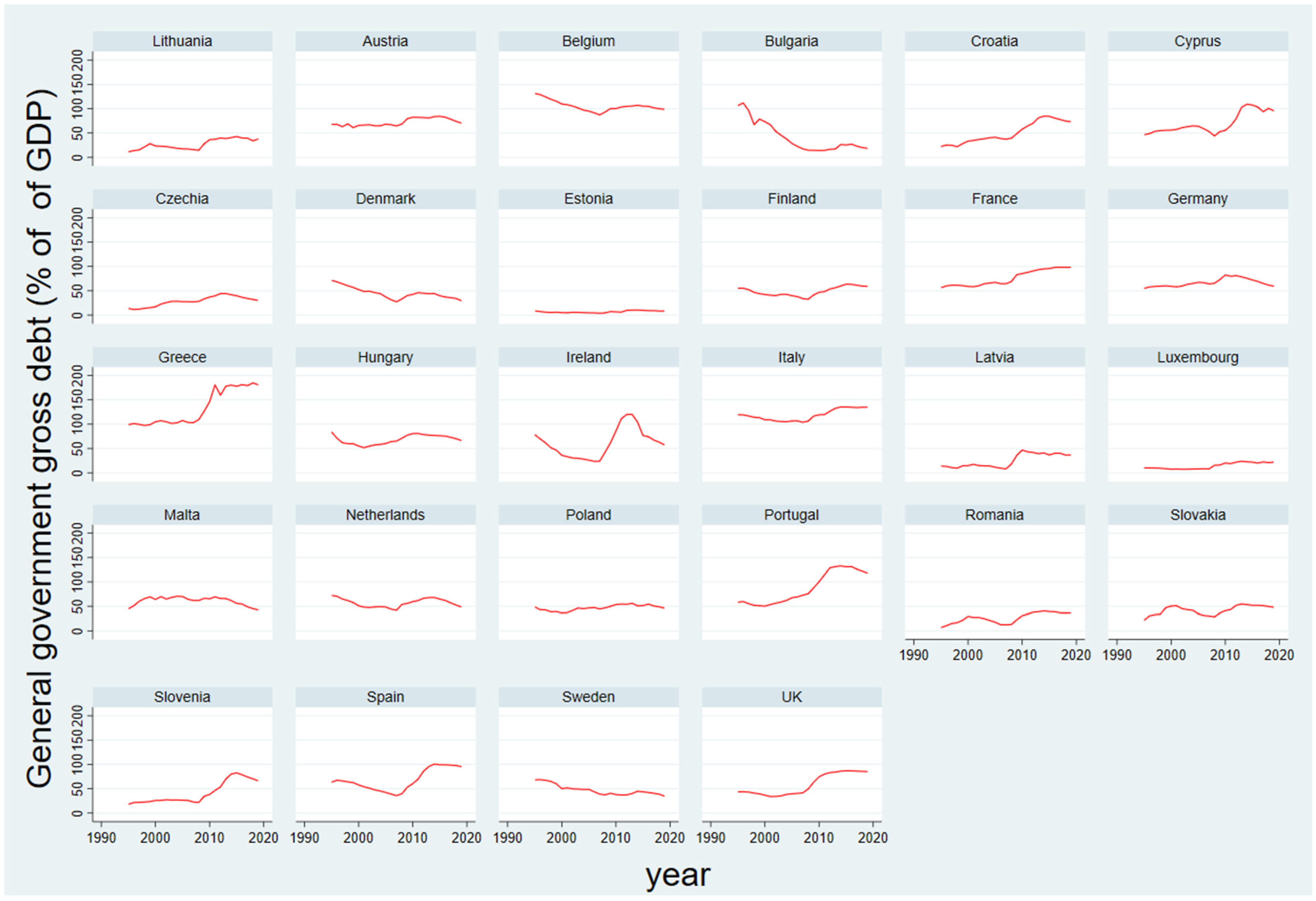
Our data consisted of 700 observations over the time span between 1995 and 2019. Because the GDP per capita was quantified in constant USD, while the other variables were usually expressed as percentages, the values were far from other statistics. We use the growth rate of GDP per capita, which has a mean of 2.51 and a standard deviation of 3.50. For the variables, the minimum value was −14.20 and the maximum was 23.90. Analyzing the dataset, we have found that 59% of debt observations (413 of 700) are below the threshold of 60%, meaning that in the specified period the EU countries had controlled the public debt level. The five most extreme values are presented in

Table 3. GDP growth and debt – the lowest and the highest values (1995–2019).

Country	Year	Real GDP per Capita Growth Rate (rgdp)	Country	Year	Public Debt (debt)
Ireland	2015	23.99	Greece	2018	184.8
Estonia	1997	14.34	Greece	2016	181.1
Latvia	2006	12.92	Greece	2019	180.9
Lithuania	2007	12.41	Greece	2011	180.6
Latvia	2005	11.95	Greece	2014	180.2
... Greece	2011	−9	Estonia	2001	4.8
Latvia	2009	−12.81	Estonia	2005	4.7
Bulgaria	1997	−13.67	Estonia	2006	4.6
Lithuania	2009	−13.86	Estonia	2008	4.5
Estonia	2009	−14.27	Estonia	2007	3.8

, showing that the maximum GDP per capita growth rate was encountered in Ireland in 2015, with a value of 23.99, while the minimum growth rate was found for Estonia in 2009, with a value of −14.27.

Regarding the debt rate, the five most extreme values were found for Greece, with the values in a range between 180 and 184, whereas the minimum values were found for Estonia, with values between 3.8 and 4.8. The data description shows that there was enough heterogeneity in the GDP per capita growth rate and in the debt rate to use the proposed methodology.

Initially, we conduct some tests that justified the use of the selected methodology. We tested the correlation among the variables to identify any possible large correlation, but also the possible relationship between growth and debt. The correlation matrix (

Table A1. Correlation matrix.

Variable	rgdp	debt	popgr	gfc	open	exp	gbb	infl
rgdp	1
debt	−0.31	1
popgr	−0.24	0.07	1
gfc	0.29	−0.47	−0.02	1
open	0.08	−0.24	0.38	0.02	1
exp	−0.39	0.45	0.11	−0.17	−0.24	1
gbb	0.26	−0.3	0.15	0.1	0.23	−0.29	1
infl	−0.16	0.01	−0.08	−0.12	−0.04	−0.12	0.01	1

) shows that no large numbers were related to the inter-dependencies among variables, while the correlation between growth and debt was negative, around 0.3, which constitutes a premise for future results; we expected the models’ coefficients to also be negative. The economic explanation is that the use of public debt negatively affects the GDP per capita rate of growth. The correlation matrix and also the variance inflation analysis shows no correlation issues (the results are available on demand).

We use different tests (Levin et al. 2002; Harris and Tzavalis 1999; Breitung and Das 2005) to determine the stationarity of the series implied. The unit root tests results are available in

Table 4. Unit root tests for the variables (testing the stationarity, with a constant).

Test Name	LLC	IPS	HT	Breitung	Hadri
Variable name: rgdp (Real GDP per capita growth rate)
Levels	−0.8665 ***	−4.6597 ***	3.2414	11.1394	71.0463 ***
First-difference	−8.1393 ***	−9.5414 ***	−21.554 ***	−11.0742 ***	−2.3987
Variable name: Debt
Levels	2.3653	−3.3451 ***	2.663	2.4499	56.5274 ***
First-difference	−7.4455 ***	−5.7161 ***	−19.8582 ***	−8.0854 ***	−2.7258
Variable name: popgr (Population growth (annual %)
Levels	−0.455 ***	−3.9554 ***	−6.7718 ***	−0.6353	26.982 ***
First-difference	−9.0981 ***	−11.8092 ***	−41.9888 ***	−9.4051 ***	−2.7444
Variable name: gfc (Gross fixed capital formation (% of GDP))
Levels	−0.8258 ***	−4.5247 ***	−3.5493 ***	−1.9773 **	28.7951 ***
First-difference	−10.4572 ***	−10.9314 ***	−33.1533 ***	−9.4087 ***	−0.8233
Variable name: open (Openness of the economy (% of GDP))
Levels	1.425	−3.3712 ***	0.8987	3.4366	65.6817 ***
First-difference	−13.2041 ***	−13.7215 ***	−36.5327 ***	−13.4128 ***	−1.9255
Variable name: ggbb (General government budget balance (% of GDP))
Levels	−5.0922 ***	−4.8364 ***	−9.9431 ***	−3.2281 ***	14.4827 ***
First-difference	−13.0814 ***	−13.2242 ***	−38.928 ***	−8.1093 ***	−2.3987
Variable name: infl (Inflation rate (annual %))
Levels	−9.299 ***	−9.0841 ***	−34.8312 ***	−1.2054	7.2403 ***
First-difference	−14.6656 ***	−21.5536 ***	−56.7277 ***	−9.8702 ***	−5.1576

Note: *** p < 0.01.

and Appendix A (

Table A2. Cointegration tests results for rgdb and debt.

Variables Name: Information about the Data (panel)	Testing Cointegration between Variables rgdp (Real GDP per Capita Growth Rate) and Debt
Test name	kao
Null hypothesis	Ho: No cointegration
Alternative hypothesis	Ha: All panels are cointegrated
Test results	Statistic	Prob	Conclusion
Modified Dickey–Fuller t	−13.0987	0.0000	Ha
Dickey–Fuller t	−10.9277	0.0000	Ha
Augmented Dickey–Fuller t	−9.8283		Ha
Unadjusted modified Dickey–Fuller	−19.1714	0.0000	Ha
Unadjusted Dickey–Fuller t	−12.1471	0.0000	Ha
Test name	Pedroni
Null hypothesis	Ho: No cointegration
Alternative hypothesis	Ha: All panels are cointegrated
Test results	Statistic	Prob	Conclusion
Modified Phillips–Perron t	−5.7096	0.0000	Ha
Phillips–Perron t	−10.0139	0.0000	Ha
Augmented Dickey–Fuller t	−10.4519	0.0000	Ha
Test name	Westerlund
Null hypothesis	Ho: No cointegration
Alternative hypothesis	Ha: All panels are cointegrated
Test results	Statistic	Prob	Conclusion
Variance ratio	−4.9577	0	Ha

). We test the cointegration between the variables using the methodology proposed by Pedroni (1999) and Westerlund (2005), using the module proposed by Khodzhimatov (2018). The cointegration between GDP and public debt was also in line with the economic literature—e.g., (Časni et al. 2014; Eberhardt and Presbitero 2015; Chirwa and Odhiambo 2020), while the panel data graphic (for every country) testifies that the series were non-stationary and co-integrated. Taking into consideration the above Equations (7) and (8), the results of

Table 5. Cointegration test results for the variables (real GDP per capita growth rate and public debt).

Cointegrated Variables Names:	rgdp (Real GDP per Capita Growth Rate), Debt (Public Debt)
Test name	Pedroni	Westerlund
MPPt	−5.7096 ***	VR	−4.9577 ***
PPt	−10.0139 ***
ADFt	−10.4519 ***

Note: *** p < 0.01.

and

Table 6. Mean group (MG), pooled mean group (PMG), and DFE results (Blackburne and Frank 2007, methodology).

Var	mg(a)	pmg(a)	dfe(a)	mg(b)	pmg(b)	dfe(b)
ECT	−0.960 ***	−0.891 ***	−0.789 ***	−1.163 ***	−0.892 ***	−0.812 ***
	(0.0466)	(0.0448)	(0.0341)	(0.0638)	(0.0454)	(0.0333)
D.debt (first lag of public Debt)	−0.484 ***	−0.479 ***	−0.306 ***	−0.191 ***	−0.234 ***	−0.247 ***
	(0.0917)	(0.0937)	(0.0209)	(0.0406)	(0.0300)	(0.0224)
debt (Public Debt)	−0.0363 ***	−0.00760 **	−0.0162 **	−0.466	−0.0117 ***	−0.0196 **
	(0.0138)	(0.00375)	(0.00782)	(0.387)	(0.00346)	(0.00915)
Obs.	672	672	.	672	672	.

Note: Standard errors in parentheses: *** p < 0.01, ** p < 0.05.

show the effects of public debt on economic growth (as a proxy, we used the real GDP per capita growth rate).

The results for the initial tests of stationarity, such as Levin et al. (2002), Im et al. (2003), Harris and Tzavalis (1999), Breitung and Das (2005), and Hadri (2000), are presented as follows (Table 4). The table is a synthesis of 80 tests (eight variables multiplied by five tests and multiplied by two cases for each one—in level and in first difference—8 × 5 × 2 = 80). For each variable, we test the stationarity to detect the presence of non-stationarity in first difference. We find that some tests suggested that the variables were stationary in levels or in first difference, so the proposed methodology could be applied. For instance, regarding the rgdp (real GDP per capita growth rate), the Harris–Tzavalis and Breitung tests suggests non-stationarity in levels (the null hypothesis of non-stationarity, stated as panels containing unit roots, cannot be rejected); further, the null of the Hadri test (“All panels are stationary”) is rejected. The variable is stationary in first difference (the null hypothesis of the Hadri test could not be rejected, while, for the other tests, the null hypothesis is rejected at a 1% level). The same logic applies for the other variables (the complete test results are available on demand). The results of the cointegration tests are provided in Table 5.

The Pedroni (1999) and Westerlund (2005) and Kao (1999) test results are presented in Table A2.

The focus of this study was the cointegration between rgdp (real GDP per capita growth rate) and debt (full results in Appendix A Table A2). From Table A2, we can see that the null hypothesis of no-cointegration was rejected. We found that all the results (modified Phillips–Perron statistic, −5.7096; Phillips–Perron statistic, −10.0139; augmented Dickey–Fuller statistic, −10.4519, variance ratio, −4.9577) were statistically significant at 1%, with the p-values at 0.000; therefore, the null was rejected and, consequently, the alternative of integration could be accepted. In Table 5 (full results in

Table A4. Cointegration test results for the variables.

Cointegrated Variable Names:	rgdp (Real GDP per Capita Growth Rate), debt (Public Debt)
Test name	Pedroni	Westerlund
MPPt	−5.7096 ***	VR	−4.9577 ***
PPt	−10.0139 ***
ADFt	−10.4519 ***
Cointegrated variable names:	rgdp (real GDP per capita growth rate), gfc (gross fixed capital formation (% of GDP))
Test name	Pedroni	Westerlund
MPPt	4.0008 ***	VR	7.0686 ***
PPt	1.1033 *
ADFt	0.7327
Cointegrated variable names:	rgdp (real GDP per capita growth rate), ggbb (general government budget balance (% of GDP))
Test name	Pedroni	Westerlund
MPPt	4.7863 ***	VR	9.326 ***
PPt	−0.904 *
ADFt	−0.4973 *
Cointegrated variable names:	rgdp (real GDP per capita growth rate), exp(general government total ex-penditure (% of GDP))
Test name	Pedroni	Westerlund
MPPt	4.6773 ***	VR	8.6163 ***
PPt	0.4928 **
ADFt	1.3037 *
Cointegrated variable names:	rgdp (real GDP per capita growth rate), infl (inflation rate (annual %))
Test name	Pedroni	Westerlund
MPPt	3.8063 ***	VR	6.6166 ***
PPt	−0.3726 *
ADFt	0.0519 *
Cointegrated variable names:	rgdp (real GDP per capita growth rate), open (openness of the economy (% of GDP))
Test name	Pedroni	Westerlund
MPPt	2.0466**	VR	−1.3862 *
PPt	−0.7558
ADFt	−1.2028
Test name	Westerlund
Cointegrated variable names:	rgdp (real GDP per capita growth rate), popgr (population growth (annual %)
Test name	Pedroni	Westerlund
MPPt	4.7301 ***	VR	7.6942 ***
PPt	−0.0553
ADFt	0.6674

Note: Standard errors in parentheses: *** p < 0.01, ** p < 0.05, * p < 0.1.

, Appendix A), we used the following abbreviations: MPPt, modified Phillips–Perron test; PPt, Phillips–Perron test; augmented Dickey–Fuller test, ADFt; variance ratio, VR.

The results suggests that the proposed methodology can control the existence of the non-stationary variables in the models. There are also some outliers present in the data, but these are also controlled in the models. The econometric literature states that, in relatively small cross-data sections, the PMG is less sensitive to outliers and the problem of autocorrelation can be corrected (Asteriou et al. 2021; Pesaran et al. 1999).

The results corresponding to equation no. 7 regarding the effects of the public debt are presented in Table 6 (full results in Appendix A,

Table A5. Mean group (MG), pooled mean group (PMG), and DFE—full results.

Var	mg(a)	pmg(a)	dfe(a)	mg(b)	pmg(b)	dfe(b)
ECT	−0.960 ***	−0.891 ***	−0.789 ***	−1.163 ***	−0.892 ***	−0.812 ***
	(0.0466)	(0.0448)	(0.0341)	(0.0638)	(0.0454)	(0.0333)
D.debt	−0.484 ***	−0.479 ***	−0.306 ***	−0.191 ***	−0.234 ***	−0.247 ***
	(0.0917)	(0.0937)	(0.0209)	(0.0406)	(0.0300)	(0.0224)
debt	−0.0363 ***	−0.00760**	−0.0162**	−0.466	−0.0117 ***	−0.0196 **
	(0.0138)	(0.00375)	(0.00782)	(0.387)	(0.00346)	(0.00915)
D.gfc				0.434 ***	0.495 ***	0.389 ***
				(0.0705)	(0.0919)	(0.0484)
D.exp				−0.149	−0.447 ***	−0.391 ***
				(0.133)	(0.0991)	(0.0761)
D.open				0.0556 **	0.0750 ***	0.0682 ***
				(0.0244)	(0.0175)	(0.0111)
D.infl				0.432 ***	0.160 ***	0.00419 *
				(0.106)	(0.0511)	(0.00224)
D.popgr				5.552 *	3.021 **	0.200
				(3.260)	(1.529)	(0.297)
D.ggbb				0.0346	−0.0969	−0.144*
				(0.126)	(0.100)	(0.0754)
gfc				−6.054	−0.000391	−0.0880*
				(6.117)	(0.0228)	(0.0477)
exp				7.959	−0.0864 ***	−0.233 ***
				(8.296)	(0.0316)	(0.0625)
open				0.353	−0.0158 ***	−0.0124 **
				(0.338)	(0.00319)	(0.00564)
infl				-11.06	−0.0390 ***	−0.0340 ***
				(10.70)	(0.00663)	(0.00386)
popgr				−2.890 **	−1.166 ***	−0.859 ***
				(1.237)	(0.150)	(0.297)
ggbb				6.521	−0.157 ***	−0.290 ***
				(6.767)	(0.0370)	(0.0701)
C	3.616 ***	2.725 ***	2.780 ***	18.47 **	7.789 ***	13.63 ***
	(0.761)	(0.245)	(0.405)	(7.311)	(0.448)	(2.560)
Obs.	672	672	.	672	672	.

Note: Standard errors in parentheses: *** p < 0.01, ** p < 0.05, * p < 0.1.

), that contains six columns, each representing the results of one model.

The first three columns display the results of the bivariate models, while the rest indicate the outcomes of the multivariate ones. We can see that, for all the models implied, the error-correction coefficient is negative, as expected, and significant. The first equation (1st column) shows the results of the mean group (the mean of the coefficients calculated for every country). The error correction term was −0.960, representing the speed of adjustment to the long-run equilibrium (the absolute value of the ECT). The coefficient suggests that deviations were corrected, at every time unit (year), by 96% (−0.960). The short-run coefficient of public debt (D.debt) was negative and statistically significant at a 1% level; therefore, in the short term, if the public debt-to-GDP ratio increases by one unit, the GDP per capita growth rate decreases by 0.484 units (percentage points), the coefficient being −0.484, ceteris paribus. In the long-run, the link is also inverse (negative), but the magnitude of the negative impact is lower. Thus, an increase in the public debt by one unit affects the rate of growth by decreasing it by 0.0363. The economic literature exhibits some models that square the debt variable, considering that a maximum value for GDP could be attained by resolving a quadratic equation (Checherita-Westphal and Rother 2012; Mencinger et al. 2014; Bilan and Ihnatov 2015; Mencinger et al. 2015; Fetai et al. 2020; Afonso and Alves 2015). However, for our data, the influence of debt on the GDP growth rate calculated in pooled values (results available on demand) did not warrant the use of a quadratic model (the figures in Appendix A.2 also confirm our decision).

In addition, based on the Hausman (1978) test, the results of the PMG (pooled mean group) estimator, which we consider to be the best approach, were in accordance with the results of the MG estimator (results available on demand). The choice of the PMG estimator is acceptable if the assumption of the long-run is not rejected, the assumption being that, in the short run, there are different responses across countries, while, in the long-run, the coefficient is restricted to exhibit non-heterogeneity. Our coefficients were statistically significant at least at a 5% level, so the assumption can be accepted.

The speed of adjustment is 0.891 (ECT = −0.891) as the coefficient was negative and significant, while the short-run growth rate decreased by 0.479 (D.debt = −0.479) and the long-run growth rate decreased by 0.007 (debt = −0.0076) The arguments for the PMG estimator are the following: the estimator allows the short run to have different values (responses) across units (countries), but restricts the long run from possessing non-heterogeneity. The DFE model shows similar results, the interpretation of the coefficients being that in the short-run, the growth rate decreased by 0.306 (−0.306) in the first model, and by 0.247 (−0.247) in the second one. The long-run coefficients also show a reduction in growth by 0.0162 (−0.0162) and 0.0196 (−0.0196), respectively.

For the multivariate models (columns from four to six), the error-correction coefficient is, again, negative and statistically significant. Following the logic above, we expect the PMG model to be the best approach; the Hausman test confirms our choice. The speed of adjustment is 0.892 (ECT = −0.892) and the short-run coefficient is −0.234, while the long-run one is −0.0117; all coefficients are significant at the 1% level. The economic interpretation is relatively similar, with the results showing that an increase in public debt has a significant negative impact on economic growth, both in the short and long term. Therefore, in both models (MG and DFE), an increase in public debt leads to a significant negative effect on economic growth. Compared to our empirical results, Gómez-Puig and Sosvilla-Rivero (2018) found that an increase in public debt could have a positive, short-term effect on economic growth, depending on the characteristics of the country and the use of the borrowed resources.

The other variables in the model, considered as control variables in the equations, were often statistically significant and had the expected sign. For example, the gross fixed capital formation, openness, inflation, and population growth exhibited significant positive short-run associations with the GDP per capita growth rate. In the long run, some of the coefficients became insignificant and some of them changed signs, but they did not impact the model findings.

To test the robustness of our results, the dataset was split into two parts, taking into consideration a first set with developed countries (dataset c; results presented in the first three columns) and a second subset with developing ones (dataset d; results presented in the last three columns). Dataset c contained the first 14 countries, sorted, by their 2019 GDP value, from the one with highest GDP value to the one with the lowest. The results for dataset c are presented in

Table 7. Mean group (MG), pooled mean group (PMG), and DFE results (Blackburne and Frank 2007, methodology) for dataset c (developed countries) and dataset d (developing countries).

Var	mg(c)	pmg(c)	dfe(c)	mg(d)	pmg(d)	dfe(d)
ECT	−1.029 ***	−0.964 ***	−0.8422 ***	−0.899 ***	−0.823 ***	−0.777 ***
	(0.080)	(0.075)	(0.046)	(0.041)	(0.034)	(0.048)
D.debt (first lag of Public Debt)	−0.403 ***	−0.401	−0.294 ***	−0.592 ***	−0.591	−0.346 ***
	(0.057)	(0.058)	(0.022)	(0.172)	(0.176)	(0.037)
debt (Public Debt)	−0.005	−0.001	0.0003	−0.0769 ***	−0.015 ***	−0.038 ***
	(0.016)	(0.004)	(0.007)	(0.020)	(0.006)	(0.013)

Note: Standard errors in parentheses: *** p < 0.01.

, where the model presented is named after the methodology and dataset used (e.g., in the first row, mg(c) indicates the results for the mean group (mg) calculated for dataset c). To obtain dataset c, the data for the following countries were separated from the initial dataset and grouped to form dataset d: Bulgaria, Croatia, Cyprus, Czech Republic, Estonia, Hungary, Latvia, Lithuania, Malta, Romania, Slovakia, Slovenia, Poland, and Portugal. The results of the bivariate model are presented in Table 7 (multivariate model results available on demand). The datasets c and d each contain 350 observations for 14 countries relative to a period of 24 years (1995–2019); the methodology proposed is pertinent.

The results in Table 7 suggest that, in developing countries, there is a more pronounced negative effect, while, in the developed countries, the long-term coefficients are close to zero but remain negative. The pmg coefficient for debt values calculated for the developed countries dataset is −0.001, which is seven times smaller than the one obtained from the analysis of the full dataset (the coefficient obtained for all data was −0.007); this indicates that the negative impact on economic growth calculated for developed countries is smaller than the one obtained for all the EU countries taken together. For the developing countries sample, the coefficient was −0.015, indicating that there is a more pronounced negative effect than that calculated for all other analyzed cases (complete dataset). Our results can be explained by the less efficient use of funds (including those obtained from extraordinary sources) in less developed (i.e., developing) countries. There are various potential factors that can explain the negative impact on growth in these countries, such as the existence of bureaucracy, less developed public institutions systems, or lower revenue rates.

The results related to our variable of interest are statistically significant in most of the models presented. However, since the ARDL method does not control the contemporaneous correlation that could appear across countries caused by unobserved factors, to demonstrate that our findings are robust, we applied the second methodology—proposed by Ditzen (2018); the final results support our previous considerations. The results based on the second methodology (effects of the public debt on growth rate, full results in

Table A6. Mean group (MG) and pooled mean group (PMG) cross-section results.

Var	mg cr(a)	pmg cr(a)	mg cr(b)	pmg cr(b)
ec ж	−0.903 ***	−0.826 ***	−1.501 ***	−1.014 **
	(0.0652)	(0.0845)	(0.105)	(0.354)
D.debt	−0.513 ***	−0.521 ***	−0.0877	−0.218 ***
	(0.0980)	(0.0952)	(0.0805)	(0.0445)
debt	−0.0404 *	−0.0203 *	−0.0448 *	−0.0249 *
	(0.0496)	(0.0176)	(0.0755)	(0.100)
D.gfc			0.491	0.369 ***
			(0.255)	(0.0953)
D.exp			−0.0803	−0.249 **
			(0.154)	(0.0749)
D.open			0.0524	0.0705 **
			(0.0599)	(0.0222)
D.infl			0.292	0.168 **
			(0.177)	(0.0615)
D.popgr			5.325	3.316
			(3.935)	(1.782)
gfc			0.0341	0.270
			(0.200)	(0.340)
exp			−0.0779	0.0846
			(0.199)	(0.362)
open			−0.0248	0.0212
			(0.0490)	(0.0952)
infl			−0.311 *	−0.108
			(0.141)	(0.295)
popgr			−2.422	−1.372
			(1.579)	(1.355)
R2	0.380	0.455	0.033	0.156
F	4.887	5.865	4.181	3.714
N	672	672	672	672

Note: ^ж we have maintained the notation used in previous tables: ec corresponds to ECT, i.e., the error-correction term. Standard errors in parentheses: *** p < 0.01, ** p< 0.05, * p < 0.1.

, Appendix A) are presented in

Table 8. Mean group (MG) and pooled mean group (PMG) cross-section results [Ditzen (2018) methodology].

Var	mg cr(a)	pmg cr(a)	mg cr(b)	pmg cr(b)
ec ж	−0.903 ***	−0.826 ***	−1.501 ***	−1.014 **
	(0.0652)	(0.0845)	(0.105)	(0.354)
D.debt (first lag of Public Debt)	−0.513 ***	−0.521 ***	−0.0877	−0.218 ***
	(0.0980)	(0.0952)	(0.0805)	(0.0445)
debt (public Debt)	−0.0404 *	−0.0203 *	−0.0448 *	−0.0249 *
	(0.0496)	(0.0176)	(0.0755)	(0.100)
R2	0.380	0.455	0.033	0.156
F	4.887	5.865	4.181	3.714
N	672	672	672	672

Note: ^ж we have maintained the notation used in previous tables: ec corresponds to ECT, i.e., the error-correction term. Standard errors in parentheses: *** p < 0.01, ** p < 0.05, and * p < 0.1.

.

The results are considering dynamic common-correlated effects, including two cross-sectional lags and instrumenting the first-lag of the dependent variable. Both the bivariate and multivariate models maintained the existence of the long-term relationship between the interest variables, as the error-correction terms are significant and negative (ec is −0.903 and −0.826 for bivariate models, mg and pmg, respectively, while, for the multivariate models, the speeds of adjustment are −1.501 and −1.014). The short-term influence is significant and negative in the bivariate models, as the coefficients have values around −0.5 (−0.513 and −0.521). In the multivariate models, the long-term influence is again significant, as the error-correction coefficients are negative, as expected. The short-run coefficients in the multivariate equations are −0.0877 and −0.218, respectively. The long-run coefficients are −0.0448 and −0.0249. The economic interpretation regarding, for example, the pmg cr (b) multivariate model, is that an increase in public debt by one unit has a negative impact on the GDP per capita rate, decreasing it by 0.0249 units, ceteris paribus.

Another caveat that could be further analyzed in future research is referring to the endogeneity due to simultaneity between growth and debt (as opposed to endogeneity due to common factors), as discussed in (Panizza and Presbitero 2014).

The same methodology was applied for the halved datasets c and d, and the results are represented in

Table 9. Mean group (MG) and pooled mean group (PMG) cross-section results [Ditzen (2018) methodology) for dataset c (developed countries) and dataset d (developing countries)].

Var	mg cr(c)	pmg cr(c)	mg cr(d)	pmg cr(d)
ec ж	−1.06 ***	−0.895 ***	−0.915 ***	−0.826 ***
	(0.114)	(0.141)	(0.111)	(0.131)
D.debt	−0.425 ***	−0.423 ***	−0.597 ***	−0.630 ***
	(0.054)	(0.058)	(0.170)	(0.177)
debt	−0.006	0.0164	−0.192	−0.054
	(0.044)	(0.030)	(0.180)	(0.094)

Note: ^ж we have maintained the notation used in previous tables: ec corresponds to ECT, i.e., the error-correction term. *** p < 0.01.

.

The results in Table 9 show that, in the short term, on the datasets implied, the results are negative and statistically significant. The negative effect is more pronounced in less developed countries (−0.597 in mg, and −0.630 in pmg, respectively), which is expected (a possible explanation being that developed economies might put funds to more efficient use). Regarding the long-term impact, most of the coefficients suggests a negative effect, but the results are not statistically significant at a 5% level. A more thorough analysis is needed in the future, when more data will become available for each country.

From a strictly economic approach, the negative impact of public debt on economic growth and on sustainable development should be a warning for public policy makers (especially in less developed countries), cautioning them on the use of this leverage. As stated in the literature (Asteriou et al. 2021), further investigation is needed to examine the possible causes of this negative impact (e.g., the inefficiency of public investments; the use of debt to cover deficits in expenditures that do not exhibit direct revenues or profits, as social expenditures; the so-called “crowding-out” effect, or generally an unwise allocation of public or private funds).

The results for all models here examined are in line with the econometric methodology and the findings of other empirical studies—e.g., (Časni et al. 2014; Afonso and Alves 2015; Asteriou et al. 2021; Lof and Malinen 2014; Chirwa and Odhiambo 2020; Pesaran et al. 1999).

5. Conclusions

The alarming increase in public debt control in various countries of the world, including EU member states, in the context of the recent and current international crisis has led to growing concerns about its economic implications. Against this background, we have witnessed a revival of researchers’ interest in assessing and analyzing the link between public debt and economic growth.

The analysis of the literature on public debt and economic growth shows that most studies have analyzed the impact of public debt on economic growth, either in the short or long term, but few studies have considered both time periods. Motivated by this, our study aimed to empirically investigate the short- and long-term impact of public debt on the economic growth in EU28 countries for a period of time covering 25 years (1995–2019). We utilized several econometric methodologies related to ARDL (autoregressive distributed lag models), such as the pooled mean group (PMG), the mean group (MG) and the dynamic fixed effects (DFE), using the methodology proposed by Blackburne and Frank in 2007, as well as the one proposed by Ditzen in 2018, which controls common-correlated effects.

In the study, we conducted tests in order to justify the use of the methodology selected, as well as tests for determining the stationarity of the series implied. In addition, we tested for cointegration between the principal variables, economic growth and public debt, and the results obtained are in line with the findings of the empirical studies mentioned in this paper.

Our empirical results, both for the bivariate models and the multivariate models, show that an increase in the public debt-to-GDP rate leads to a decrease in the real GDP per capita growth rate in EU28 countries, both in the short and long term. Specifically, the estimated public debt coefficients appear statistically significant and negative, but the magnitude of the negative impact on economic growth differs significantly. These findings are of interest because a high and persistent level of public debt can have detrimental effects on the accumulation of capital and productivity, which reduces economic growth. To test the robustness of our results, the dataset was split into two parts, namely, a first set including developed countries and a second subset including developing ones. Our empirical results suggest that, both in the short and long term, public debt is negatively correlated with economic growth in the case of developing countries. Comparatively, in the case of developed EU countries, the effect in the long run is in general negative, but statistically insignificant. Our results can be explained by the less efficient use of funds in less developed (i.e., developing) countries. Further, there are some potential factors that can explain the negative impact on growth in these countries (e.g., the existence of bureaucracy, poor quality of the institutional environment, or reduced allocation to investments).

On the whole, the findings of our empirical investigation confirm the conclusions of some previous empirical studies which focused on evaluating the impact of public debt on economic growth, both in the short and long term.

Our empirical findings suggest that public debt is a significant predictor of economic growth; thus, public policies aimed at stimulating economic growth should take into account the level of public debt and control it. Furthermore, the rigorous monitoring/control of the level of public debt is of major importance, as ensuring this, maintains a long-term downward trajectory that will sustain economic growth.

Regarding future research directions, we aim to continue our research by identifying the channels through which public debt affects economic growth. We also aim to examine the role of the quality of institutions in the relationship between public debt and economic growth.

References

- Afonso, Antonio, and José Alves. 2015. The Role of Government Debt in Economic Growth, Hacienda Pública Española. Review of Public Economics 215: 9–26. [Google Scholar]
- Albu, Ada-Cristina, and Lucian Liviu Albu. 2021. Public debt and economic growth in Euro area countries. A wavelet approach. Technological and Economic Development of Economy 27: 602–25. [Google Scholar] [CrossRef]
- Asteriou, Dimitrios, Keith Pilbeam, and Cecilia Eny Pratiwi. 2021. Public debt and economic growth: Panel data evidence for Asian countries. Journal of Economics and Finance 45: 270–87. [Google Scholar] [CrossRef]
- Baum, Anja, Cristina Checherita-Westphal, and Philipp Rother. 2013. Debt and growth: New evidence for the euro area. Journal of International Money and Finance 32: 809–21. [Google Scholar] [CrossRef] [Green Version]
- Bentour, El Mostafa. 2021. On the public debt and growth threshold: One size does not necessarily fit all. Applied Economics 53: 1280–99. [Google Scholar] [CrossRef]
- Bilan, Irina, and Iulian Ihnatov. 2015. Public Debt and Economic Growth: A wo-Sided Story. International Journal of Economic Sciences 4: 24–39. [Google Scholar] [CrossRef]
- Blackburne, Edward F., III, and Mark W. Frank. 2007. Estimation of nonstationary heterogeneous panels. The Stata Journal 7: 197–208. [Google Scholar] [CrossRef]
- Breitung, Jörg, and Samarjit Das. 2005. Panel unit root tests under cross-sectional dependence. Statistica Neerlandica 59: 414–33. [Google Scholar] [CrossRef]
- Butkus, Mindaugas, Diana Cibulskiene, Lina Garsviene, and Janina Seputiene. 2021. The Heterogeneous Public Debt–Growth Relationship: The Role of the Expenditure Multiplier. Sustainability 13: 4602. [Google Scholar] [CrossRef]
- Časni, Anita Čeh, Ana Andabaka Badurina, and Martina Basarac Sertić. 2014. Public debt and growth: Evidence from Central, Eastern and Southeastern European countries. Proceedings of Rijeka Faculty of Economics, Journal of Economics and Business 32: 35–51. [Google Scholar]
- Checherita-Westphal, Cristina, and Philipp Rother. 2012. The impact of high government debt on economic growth and its channels: An empirical investigation for the euro area. European Economic Review 56: 1392–405. [Google Scholar] [CrossRef]
- Chirwa, Themba Gilbert, and Nicholas M. Odhiambo. 2020. Public debt and economic growth nexus in the Euro area: A dynamic panel ARDL approach. Scientific Annals of Economics and Business 67: 291–310. [Google Scholar] [CrossRef]
- Choi, In. 2001. Unit root tests for panel data. Journal of International Money and Finance 20: 249–72. [Google Scholar] [CrossRef]
- Chudik, Alexander, and M. Hashem Pesaran. 2013. Large Panel Data Models with Cross-Sectional Dependence: A Survey. Globalization Institute Working Papers. Dallas: Federal Reserve Bank of Dallas. [Google Scholar]
- Chudik, Alexander, and M. Hashem Pesaran. 2015. Common correlated effects estimation of heterogeneous dynamic panel data models with weakly exogenous regressors. Journal of Econometrics 188: 393–420. [Google Scholar] [CrossRef] [Green Version]
- Chudik, Alexander, Kamiar Mohaddes, M. Hashem Pesaran, and Mehdi Raiss. 2017. Is there a debt-threshold effect on output growth? Review of Economics and Statistics 99: 135–50. [Google Scholar] [CrossRef] [Green Version]
- Dickey, David A., and Wayne A. Fuller. 1979. Distribution of the estimators for autoregressive time series with a unit root. Journal of the American Statistical Association 74: 427–31. [Google Scholar]
- Ditzen, Jan. 2018. Estimating dynamic common-correlated effects in Stata. The Stata Journal 18: 585–617. [Google Scholar] [CrossRef]
- Eberhardt, Markus, and Andrea F. Presbitero. 2015. Public debt and growth: Heterogeneity and non-linearity. Journal of International Economics 97: 45–58. [Google Scholar] [CrossRef]
- Égert, Balázs. 2015. Public debt, economic growth and nonlinear effects: Myth or reality? Journal of Macroeconomics 43: 226–38. [Google Scholar] [CrossRef] [Green Version]
- Fetai, Besnik, Kestrim Avdimetaj, Abdylmenaf Bexheti, and Arben Malaj. 2020. Threshold effect of public debt on economic growth: An empirical analysis in the European transition countries. Zbornik Radova Ekonomski Fakultet u Rijeka 38: 381–406. [Google Scholar]
- Gómez-Puig, Marta, and Simón Sosvilla-Rivero. 2017. Heterogeneity in the debt-growth nexus: Evidence from EMU countries. International Review of Economics & Finance 51: 470–86. [Google Scholar]
- Gómez-Puig, Marta, and Simón Sosvilla-Rivero. 2018. Public debt and economic growth: Further evidence for the Euro area. Acta Oeconomica 68: 209–29. [Google Scholar] [CrossRef] [Green Version]
- Hadri, Kaddour. 2000. Testing for stationarity in heterogeneous panel data. The Econometrics Journal 3: 148–61. [Google Scholar] [CrossRef]
- Harris, Richard D. F., and Elias Tzavalis. 1999. Inference for unit roots in dynamic panels where the time dimension is fixed. Journal of Econometrics 91: 201–26. [Google Scholar] [CrossRef]
- Hausman, Jerry A. 1978. Specification tests in econometrics. Econometrica 46: 1251–71. [Google Scholar] [CrossRef]
- Herndon, Thomas, Michael Ash, and Robert Pollin. 2013. Does high public debt consistently stifle economic growth? A Critique of Reinhart and Rogoff 38: 263–66. [Google Scholar]
- Im, Kyung So, M. Hashem Pesaran, and Yongcheol Shin. 2003. Testing for unit roots in heterogeneous panels. Journal of Econometrics 115: 53–74. [Google Scholar] [CrossRef]
- Jacobs, Jan, Kazuo Ogawa, Elmer Sterken, and Ichiro Tokutsu. 2020. Public debt, economic growth and the real interest rate: A panel VAR Approach to EU and OECD countries. Applied Economics 52: 1377–94. [Google Scholar] [CrossRef]
- Kao, Chihwa. 1999. Spurious regression and residual-based tests for cointegration in panel data. Journal of Econometrics 90: 1–44. [Google Scholar] [CrossRef]
- Khodzhimatov, Ravshanbek. 2018. XTCOINTREG: Stata module for panel data generalization of cointegration regression using fully modified ordinary least squares, dynamic ordinary least squares, and canonical correlation regression methods. In Statistical Software Components. Boston: Boston College Department of Economics. [Google Scholar]
- Kourtellos, Andros, Thanasis Stengos, and Chih Ming Tan. 2013. The effect of public debt on growth in multiple regimes. Journal of Macroeconomics 38: 35–43. [Google Scholar] [CrossRef] [Green Version]
- Kumar, Manmohan S., and Jaejoon Woo. 2010. Public debt and growth. IMF Working Paper 174: 1–46. [Google Scholar] [CrossRef] [Green Version]
- Law, Siong Hook, Chee Hung Ng, Ali M. Kutan, and Zhi Kei Law. 2021. Public debt and economic growth in developing countries: Nonlinearity and threshold analysis. Economic Modelling 98: 26–40. [Google Scholar] [CrossRef]
- Levin, Andrew, Chien-Fu Lin, and Chia-Shang James Chub. 2002. Unit root tests in panel data: Asymptotic and finite-sample properties. Journal of Econometrics 108: 1–24. [Google Scholar] [CrossRef]
- Liu, Zhongmin, and Jia Lyu. 2021. Public debt and economic growth: Threshold effect and its influence factors. Applied Economics Letters 28: 208–12. [Google Scholar] [CrossRef]
- Lof, Matthijs, and Tuomas Malinen. 2014. Does sovereign debt weaken economic growth: A panel VAR analysis. Economics Letters 122: 403–7. [Google Scholar] [CrossRef] [Green Version]
- Masuch, Klaus, and Edmund Moshammer. 2017. Institutions, public debt and growth in Europe. Public Sector Economics 41: 160–205. [Google Scholar] [CrossRef]
- Mencinger, Jernej, Aleksander Aristovnik, and Miroslav Verbič. 2014. The impact of growing public debt on economic growth in the European Union. Amfiteatru Economic Journal 16: 403–14. [Google Scholar]
- Mencinger, Jernej, Aleksander Aristovnik, and Miroslav Verbič. 2015. Revisiting the role of public debt in economic growth: The case of OECD countries. Engineering Economics 26: 61–66. [Google Scholar] [CrossRef] [Green Version]
- Newey, Whitney K., and Kenneth D. West. 1987. Hypothesis testing with efficient method of moments estimation. International Economic Review 28: 777–87. [Google Scholar] [CrossRef]
- Panizza, Ugo, and Andrea F. Presbitero. 2013. Public Debt and Economic Growth in Advanced Economies: A Survey. Swiss Journal of Economics and Statistics 149: 175–204. [Google Scholar] [CrossRef] [Green Version]
- Panizza, Ugo, and Andrea F. Presbitero. 2014. Public debt and economic growth: Is there a causal effect? Journal of Macroeconomics 41: 21–41. [Google Scholar] [CrossRef] [Green Version]
- Pattillo, Catherine A., Helene Poirson, and Luca A. Ricci. 2004. What Are the Channels through Which External Debt Affects Growth? IMF Working Paper No. 04/15. Washington, DC: International Monetary Fund. [Google Scholar]
- Pedroni, Peter. 1999. Critical values for cointegration tests in heterogeneous panels with multiple regressors. Oxford Bulletin of Economics and Statistics 61: 653–70. [Google Scholar] [CrossRef]
- Pesaran, M. Hashem, Yongcheol Shin, and Ron P. Smith. 1999. Pooled mean group estimation of dynamic heterogeneous panels. Journal of the American statistical Association 94: 621–34. [Google Scholar] [CrossRef]
- Pescatori, Andrea, Damiano Sandri, and John Simon. 2014. No magic threshold. Finance & Development 51: 39–42. [Google Scholar]
- Phillips, Peter C. B., and Pierre Perron. 1988. Testing for a unit root in time series regression. Biometrika 75: 335–46. [Google Scholar] [CrossRef]
- Rahman, Nur Hayati Abd, Shafinar Ismail, and Abdul Rahim Ridzuan. 2019. How does public debt affect economic growth? A systematic review. Cogent Business & Management 6: 1–16. [Google Scholar]
- Ramos-Herrera, María del Carmen, and Simón Sosvilla-Rivero. 2017. An empirical characterization of the effects of public debt on economic growth. Applied Economics 49: 3495–508. [Google Scholar] [CrossRef]
- Reinhart, Carmen, and Kenneth S. Rogoff. 2010a. Growth in a time of debt. American Economic Review 100: 573–78. [Google Scholar] [CrossRef] [Green Version]
- Reinhart, Carmen, and Kenneth S. Rogoff. 2010b. Debt and growth revisited. MPRA Paper No. 24376. Available online: https://mpra.ub.uni-muenchen.de/24376/1/Debt_and_Growth_Revisited.pdf (accessed on 10 July 2022).
- Sutherland, Douglas, and Peter Hoeller. 2012. Debt and Macroeconomic Stability: An Overview of the Literature and Some Empirics. OECD Economics Department Working Papers, No. 1006. Paris: OECD Publishing. [Google Scholar]
- Vanlaer, Vanlaer, Marneffe Willem, Vereeck Wim, and Johan Lode Vanovertveldt. 2015. Does debt predict growth? An empirical analysis of the relationship between total debt and economic output. European Journal of Government and Economics 4: 79–103. [Google Scholar] [CrossRef]
- Westerlund, Joakim. 2005. New simple tests for panel cointegration. Econometric Reviews 24: 297–316. [Google Scholar] [CrossRef]