Abstract
Radial symmetry, by our definition, is a precise condition on continuous ideal-point distributions, rarely if ever found exactly in practice, that is similar to the classical 1967 symmetry condition of Plott but pertains to an infinite electorate; the bivariate normal distribution provides an example. A Condorcet cycle exists if the electorate prefers alternative X to Y, Y to Z, and Z to X. An alternative K is a Condorcet winner if there is no alternative that the electorate prefers to K. Lack of a Condorcet winner may engender turmoil. The nonexistence of a Condorcet winner implies that a Condorcet cycle exists. Radial symmetry precludes the existence of Condorcet cycles and thus guarantees a Condorcet winner; but this result assumes that all voters weight the dimensions alike. Our counterexamples show that a Condorcet cycle can arise, even under radial symmetry, if the weighting of issues varies across voters. This finding may be of more than theoretical value: It may suggest that in an empirical setting (without radial symmetry), a Condorcet cycle may be more frequent if voters differ as to how they weight the dimensions. We examine, for illustration based on two dimensions (left–right, linguistic), a Condorcet preference cycle in Finland’s 1931 presidential election.
1. Introduction
An election or vote may breed discord if there is no Condorcet winner—if every alternative faces at least one competing alternative that the electorate (strictly) prefers. That quandary reflects a Condorcet cycle, where (more than half of) the electorate prefers alternative X to Y, Y to Z, and Z to X.
We define a symmetry condition, which we refer to as radial symmetry, that is similar to that in the classic work of Plott (1967) (and is a large-electorate analog thereof) but involves an infinite (rather than finite) number of voters along with a continuous distribution of voter ideal points. Similar to Plott’s condition, it is highly restrictive.
It precludes a Condorcet cycle among any three alternatives (thus guaranteeing a Condorcet winner) if all voters weight the issues alike. However, such is no longer the case if voters differ as to the relative importance they attach to the issues, as we show using counterexamples with two dimensions (issues). This interesting theoretical finding may have practical implications: It may suggest that, correspondingly, Condorcet cycles are more likely empirically if voters weight the issues disparately. Dimensions that may be afforded different relative importance by different political parties or voters may include economic left–right, social–cultural, and others (see, e.g., Polk et al. 2017). Of course, the extent to which Condorcet cycles have real-world relevance in the first place has been questioned, as in Tullock (1967). Simpson (1969) amplifies Tullock’s (1967) work and mentions Plott’s (1967) condition.
Our work here has several distinguishing features. (i) Its model deals with differential issue weightings among voters, a facet of spatial modeling that is not often recognized in prior literature. (ii) Its model uses a continuous distribution of ideal points with an infinite number of voters, in contrast to the setup with a finite number of voters that is generally specified under the Plott (1967) model. This infinite-electorate model not only bears greater resemblance to the real world of voters in large public elections but also has certain advantages of lucidity. (iii) For the case where issue weightings are the same for all voters, the continuous distribution of ideal points with an infinite electorate leads to a simpler proof of the result—akin to the classical one under the Plott model—that radial symmetry precludes Condorcet cycles. (iv) For the case where issue weightings differ among voters, we focus on showing that radial symmetry does not preclude Condorcet cycles under the infinite-electorate setup but also find that that conclusion holds under the Plott finite-electorate model as well. This primary result of ours is expressed in the title of the paper. (v) In addition to their theoretical interest, our results may have the practical implications indicated in the preceding paragraph: They may suggest a hypothesis that cycles are more apt to occur with greater weighting differences among voters.
In what follows, Section 2 covers the details of our setting and concepts. For the case where voters’ weightings are homogeneous and the electorate is infinite, propositions for radial symmetry established in Section 3 have simpler proofs and stronger results than comparable ones for a finite electorate with their standard symmetry conditions.
A limited discussion of earlier writings on differential weightings is in Section 4. This review of prior results covers a short note (Hoyer and Mayer 1975) that presents a finite-electorate example with radial symmetry where a Condorcet cycle occurs under differential weighting, though with an atypical set of utility functions.
For the case (under radial symmetry) where the voter weightings differ from one another, only one counterexample is needed to prove that Condorcet cycles are not precluded. Nonetheless, Section 5 provides several of them to illustrate different ways in which the cycles can occur for an infinite electorate; Section 6 covers the case of a finite electorate.
2. Framework
We start by defining our framework, which is similar, but not identical, to that of Plott (1967; hereafter Pl); is even closer to that of Feld and Grofman (1987, especially Theorem 6; hereafter F-G) and Miller (2015, especially p. 172; hereafter Mi); and has still more common elements with Davis et al. (1972; hereafter DD&H). As we lay out our framework below, we indicate differences between it and Pl, F-G, Mi, and DD&H. (Note, though, that the second and third framework items below obviously do not apply to Section 6 below.)
Dimensions. We work with an issue space of two dimensions, but results are generally extendable to more than two.
Voters. We have an infinite number of voters (which closely approximates a large electorate). Each voter V has a (unique) ideal point, where V’s utility is maximal. By contrast, Pl, F-G, and Mi use a finite number of voters, though they can be located in varying ways. DD&H allow for either a finite or an infinite electorate.
Distribution of voters’ ideal points. We posit that this ideal-point distribution is continuous. It is discrete for Pl, F-G, and Mi (since their number of voters is finite). DD&H provide for it to be either discrete or continuous. Use of a continuum of voters in voting applications is also found in (e.g.) Caplin and Nalebuff (1988, p. 789).
Alternatives. Alternatives, or options, could be political candidates, legislative proposals, or something else. Hereafter, we will just refer to the alternatives as candidates but with the understanding that other possibilities are not precluded. Candidates’ (unique) ideal points are located in the same issue space as those of voters. Our counterexamples use three candidates, though similar ones with more than three could easily be constructed. Pl, F-G, and Mi do not consider triples of candidates (or of other alternatives) in the way that we do. DD&H have two examples that use three alternatives.
Utility function. We write PV: (xV, yV) for the ideal point of voter V and PG: (xG, yG) for the ideal point of candidate G. Our utility function is negative squared Euclidean distance for the case where all voters weight the two issues alike, so that the utility of voter V for candidate G is
For F-G, Mi, and DD&H, utility is also based on Euclidean distance, but for Pl it involves the utility gradient because the Pl treatment is more general.
Disparate weighting of issues. For the case where voters differ in their relative weightings of the two issues, we generalize (1) and use the utility function
Weight ratios : of 6:3, 2:1, and 1:½ (e.g.) all have the same effect. (Suitable weight ratios will vary depending on the relative scaling of x and y.) In general, the weight ratios : follow a distribution that can vary with (i.e., can be conditional on) the point PV: (xV, yV). However, for our counterexamples later, except those in Section 6, the : weight ratios have the same distribution for the voters at every point (xV, yV) in the issue space (e.g., a distribution that, at each point, assigns 1:9 for half the voters and 9:1 for the other half). Accordingly, with the : distribution independent of the ideal point PV, it is designated more simply as the w1:w2 distribution. (We can create each type of counterexample in Section 5 without a need for the : distribution to differ for different PV.) Pl, F-G, Mi, and DD&H do not consider different weightings of the dimensions by different voters and so do not deal with anything like (2).
Radial symmetry. We define radial symmetry to be present in the distribution of voter ideal points if there exists a point M such that every line that passes through M has half the voters on each side of the line. (Because the distribution is continuous, points that are on the line itself can be disregarded.) Without loss of generality, we assume M to be the origin, (0, 0). Note that, with our framework, the definition of radial symmetry pertains only to the distribution of voters’ ideal points and says nothing about a utility function (or about weighting of issues, or about the candidates). F-G and Mi do not use the term radial symmetry but, for a discrete distribution of voter ideal points, have a concept that can be deemed analogous to ours: There is a voter at M, and every line through M has the same number of voters on each side of M. The framework of Pl is also analogous but is more general and does involve utility. DD&H use concepts similar to ours.
Condorcet cycles. Under (1), our definitions that follow are consonant with standard ones and with those of Pl, F-G, Mi, and DD&H. Voter V at point PV: (xV, yV) prefers candidate G at PG: (xG, yG) to candidate H at PH: (xH, yH) if and only if U(V, G) > U(V, H). We write G►H to denote that more than half the electorate prefers G to H. (G►H if and only if more than half the electorate has greater utility for G than for H (i.e., is closer to PG than to PH, or, equivalently, is on the PG side of the perpendicular bisector of the line segment joining PG and PH).) We define a Condorcet cycle to exist among three candidates A, B, and C if A►B, B►C, and C►A; or if B►A, C►B, and A►C. We then define preclusion of Condorcet cycles to mean that it is not possible to choose, from anywhere in the issue space, a triple of candidates A, B, and C that exhibits a Condorcet cycle. If, in a group of existing candidates, A is a(n existing) candidate such that G►A (A►G) for no other (existing) candidate G located elsewhere, then A is a Condorcet winner (Condorcet loser). Under (2) with the weight ratio following the same distribution throughout the space of voter ideal points, definitions akin to the foregoing apply.
Miscellaneous. We mention three further details. First, although we use straightforward definitions of Condorcet winner and Condorcet loser, it should be noted that (rarely) there can be more than one of either (e.g., two Condorcet winners, X and Y, will exist if the preference ranking is XYZ for half the electorate and YXZ for the other half). Second, although the absence of a Condorcet winner implies the presence of a Condorcet cycle, the converse is not true (e.g., B►C, C►D, and D►B, but A►B, A►C, and A►D). Third, we refrain from dealing with concepts such as the core (e.g., Saari 1997; Schofield 2008) that are closely related to Condorcet winners but are not essential to our development here.
3. Radial Symmetry as a Sufficient Condition to Preclude Condorcet Cycles under (1)
For (1) for our framework above, we state and prove three propositions.
Proposition 1.
Condorcet cycles are precluded if radial symmetry holds.
Proof.
For two candidates G at (xG, yG) and H at (xH, yH), define
which are the respective squares of their distances from the origin (i.e., from M). We start by showing that G►H if and only if .
A voter V at (xV, yV) prefers G to H if and only if or if and only if
or if and only if
The line that bounds the region (3) is parallel to the line that bounds
However, the latter line passes through the origin and so, by the assumption of radial symmetry, has half the electorate on each side of it. The region defined by (3) (which is the set of voters V who prefer G to H) is larger than the region defined by (4) if and only if . Thus, G►H if and only if , since the latter region contains half the electorate.
To complete the proof, consider any three candidates A, B, and C whose respective squared distances from the origin are ,, and . It is, of course, not possible for these three values to exhibit intransitivity, so a Condorcet cycle among A, B, and C cannot occur. □
Although Proposition 1 and its proof are only for two dimensions, we remark that extension to more than two dimensions is immediate. Note also that it is easy to extend the proof to preclude any cyclicity among any group of more than three candidates.
Proposition 2.
If (given radial symmetry) any set of candidates includes a candidate K located at M (the origin), then K is a Condorcet winner.
Proof.
Follows at once from the foregoing, by noting that . □
Proposition 2 can be considered an analog, for continuous ideal-point distributions, of the basic result of Pl, F-G, and Mi (for discrete distributions) that proves that a Condorcet winner, located at the origin, must exist under their symmetry conditions. Not only is Proposition 2 unusual in this setting in that it pertains to continuous rather than discrete ideal-point distributions, but also its proof has the benefit of being comparatively simple.
Proposition 3.
Radial symmetry guarantees a Condorcet winner even if there is no candidate located at the origin.
Proof.
This result, stronger than Proposition 2, follows from Proposition 1 because the impossibility of any Condorcet cycles implies the existence of a Condorcet winner. □
Curiously, as a matter of theoretical interest, and in contrast to the finite-electorate setup, Proposition 3 functions even if no voter is located at the origin. For example, in the distribution of voter ideal points there could be a doughnut hole centered at the origin.
The possible pedagogical value of the above results should not be overlooked. In particular, the proof of Proposition 1, under a continuous distribution of ideal points, is shorter and more straightforward than corresponding proofs under discrete distributions. Related results and proofs in DD&H, however, do apply to a continuous ideal-point distribution and an infinite electorate and are similar (though not identical) to ours above. Our development may be less comprehensive, but also more understandable, than that of DD&H.
We note that Propositions 1–3 still hold under a special case of (2) in which , are replaced by , such that the weights are the same for all voters at a given point (as well as from one point to another) but can still differ between the two issues. This is just a transformation of scale: If we substitute and into the modified (2), then x0 and y0 satisfy (1), and radial symmetry still holds after the transformation.
4. Previous Work That Has Considered Unequal Weighting
Thus far, we have concentrated on the case where all voters weight the issues alike. For utility functions, whether with or without radial or other symmetry in the ideal-point distributions that apply, most authors do not consider cases where voters differ as to how they weight the dimensions. However, such differences in weighting are central to the present paper.
In earlier work, Davis and Hinich (1968, p. 68) treat a situation where some voters care only about a single issue (which may vary from one voter to another). Although Davis et al. (1970, p. 434) refer to but eschew a model with different weights for different voters, they do briefly mention that a voter may care about only one issue (p. 433), that farmers may care especially about farm price supports and petroleum-industry people about oil import quotas (p. 440), and that an assumption of equal weighting is not generally satisfied (p. 446). Hoyer and Mayer (1974) provide extensive comparisons of a model where all voters have the same weighting versus a model where voter weightings can differ. Hinich and Pollard (1981) use a model that allows voters to differ not only in their weightings of issues but also in their perceptions of candidates’ positions on issues. Each candidate is located along a single “predictive dimension” (though more than one such dimension may be possible). Rabinowitz et al. (1982), Niemi and Bartels (1985), and Erikson and Romero (1990) consider weighting differences that are associated with differences in the saliences that voters attach to issues. Rivers (1988, p. 740) disapproves that voter heterogeneity in issue weighting is ignored “in common practice,” before developing an approach that handles it. Although the utility function in the model of Adams (1997, p. 1254) allows for differences among voters as to how they weight the dimensions, that flexibility is not put to use. Adams and Adams (2000, p. 140) mention the possibility that “different policy dimensions matter to different voters” but judge that such a point does not affect their conclusions. Feld et al. (2014, pp. 480–81) briefly allude to a possible model “that would allow variation in the salience different voters attach to different issues.”
Unlike the references just cited, Hoyer and Mayer (1975, p. 806) provide an example, for a finite electorate, where a Condorcet cycle occurs with radial symmetry and weighting differences among voters. That example has three candidates and nine voters. Though it is presented geometrically rather than algebraically, its utility functions do not all conform to (2) above. They do so for three of the nine voters. For the other six, however, the utility function is the same as (2) but with an added cross-product term of the form .
5. With an Infinite Electorate, Radial Symmetry, and Unlike Weighting, Cycles Can Occur
For an infinite electorate, we next provide counterexamples to establish that, even with (unlikely) radial symmetry of the distribution of voter ideal points, preclusion of Condorcet cycles is not guaranteed if voters differ (in their utility functions) as to the comparative importance they attach to the issues in the policy space. Even given the tight radial-symmetry restrictions, some critics might still find this result unsurprising. Here, we are proving the result by counterexample to provide broad insights, although other methods of proof might be used. Even though with equal weighting slight perturbances from radial symmetry are sufficient to create a Condorcet cycle, our counterexamples with unequal weighting (and radial symmetry) were not easy to construct, rest on thin margins for some candidate pairings, and (in most cases) place all or almost all of a given voter’s weight on just one of the two issues.
We consider two bivariate (infinite-electorate) ideal-point distributions that observe radial symmetry. The first is a bivariate normal distribution with a mean of 0 and standard deviation of 10 for both x and y; we use a correlation coefficient of 0 (although, even if it is not 0, radial symmetry still holds). The second is a uniform (rectangular) distribution with probability density function f(x, y) = 1/400 over the square with vertices (x, y) = (−10, 10), (10, 10), (−10, −10), and (10, −10).
A single counterexample would suffice to show that Condorcet cycles are no longer precluded for voter ideal-point distributions with radial symmetry in an infinite electorate if voters differ as to how they judge the relative importance of the issues. We provide several counterexamples, however, in order to illustrate particular features.
Examples 1.1 and 1.2. The respective spatial locations of candidates A, B, and C are
If all voters have the same utility function, as in (1), then A►B, B►C, and A►C since ,, and (no cycle).
PA: (xA, yA) = (1, 7); PB: (xB, yB) = (3, −7); and PC: (xC, yC) = (−9, 5).
However, now suppose instead that (at each point in the issue space) half the electorate attaches sole importance to the issue on the x-axis whereas the other half cares only about the y-dimension. The utility functions (of voter V for candidate G) can then be represented by (2) with respective weight ratios w1:w2 of 1:0 and 0:1.
Example 1.1.
If the ideal points follow the uncorrelated bivariate normal distribution indicated above, then A►B, B►C, and C►A, so a Condorcet cycle exists. See Appendix A.1 for calculation details.
Example 1.2.
Suppose now that the distribution of ideal points is uniform (as described above) rather than bivariate normal. Then a Condorcet cycle exists again, once more with A►B, B►C, and C►A. Here, the margins by which the electorate prefers A over B, B over C, and C over A are identical: 55% to 45% in all three cases. See Appendix A.1 for calculation details.
In Examples 1.1–1.2, as well as below in Examples 3.1–3.2 and in parts of Example 4, each voter is concerned about only one of the two issues. Those examples were constructed in that way to provide ease of exposition and calculation.
It might be claimed, though, that all these counterexamples are problematic because the concern of voters for only one dimension renders the setting unidimensional rather than truly two-dimensional. Although we find it hard to grant that this is a valid objection, we nonetheless counter by pointing out that the proportion of the electorate with G►H (for two candidates G and H) can be a continuous—not discontinuous—function of the weight ratios. Thus, a change in the weight ratios from 1:0 and 0:1 to 1:ε and ε:1, for tiny enough ε, will not break the cycle. In fact, ε does not (in general) even need to be tiny, as evidenced by the next example.
Example 2.
The same cycle as in Examples 1.1–1.2 (A►B, B►C, C►A) also occurs if (e.g.) Example 1.2 is unchanged except that all voters care (somewhat) about both dimensions with weight ratios w1:w2 of 10:1 and 1:10 in place of 1:0 and 0:1. The (complicated) calculation details are in Appendix A.2.
Examples 3.1 and 3.2. For candidates A, B, and C, respective locations are
With the same utility function for all voters as in (1), no cycle can exist: A►B, B►C, and A►C, with ,, and . However, suppose now that, as in Examples 1.1–1.2, weightings differ across voters according to (2) with weight ratios w1:w2 of 1:0 for half the electorate and 0:1 for the other half.
PA: (xA, yA) = (−3, 9); PB: (xB, yB) = (7, 7); and PC: (xC, yC) = (5, −9).
Example 3.1.
If the ideal points follow the uncorrelated bivariate normal distribution, a Condorcet cycle occurs with B►A, C►B, and A►C. See Appendix A.3 for calculation details.
Example 3.2.
If the ideal points follow the uniform rather than the bivariate normal distribution, a Condorcet cycle exists again, also with B►A, C►B, and A►C. See Appendix A.3 for calculation details.
Note that, even though Examples 1.1–1.2 and 3.1–3.2 all have A►B, B►C, and A►C if all voters have the same utility function, with the change to 1:0 and 0:1 Examples 1.1–1.2 have the cycle A►B, B►C, and C►A whereas the cycle in Examples 3.1–3.2 is the opposite—B►A, C►B, and A►C. Thus, interestingly, only A►C is reversed in the former case, but both A►B and B►C are reversed in Examples 3.1–3.2—a salient difference between the two cases.
Example 4.
We extend Example 3.2, still with the same uniform distribution for the ideal points and the same three candidates, but now we suppose that the weight ratios w1:w2 for (2) are 1:0 for only 6% of the voters, 0:1 for another 6%, and 1:1 (equal weighting) for the remaining 88%. Even though an overwhelming proportion of the voters (88%) are identical with one another as to how they weight the issues, it turns out that the Condorcet cycle with B►A, C►B, and A►C nonetheless emerges again. See Appendix A.4 for calculation details. Therefore, here, even with radial symmetry, the generation of a cycle does not require a very large fraction of voters with non-conforming weightings.
Obviously, where radial symmetry holds, many possible cases of unlike voter weightings of issues will not serve to trigger Condorcet cycles. The above counterexamples serve simply to establish the possibility of those cycles.
In all of those counterexamples, the distribution of the weight ratios : is the same (set at w1:w2) for voters at every point in the issue space (e.g., 10:1 for half the voters at each point and 1:10 for the other half). This allows for easier presentation but also shows that counterexamples need not be made more elaborate through use of different distributions at different points. Because of similar considerations, all of our chosen weight ratio distributions are discrete (in fact, mostly dichotomous) rather than continuous, although a possible continuous weight-ratio distribution is described briefly just before Table A1 in Appendix A.2 below.
6. Counterexamples for the Case of a Finite Electorate
Although this paper concentrates on establishing that Condorcet cycles are not precluded with differential weighting under radial symmetry if the number of voters is infinite, a comparable result holds for a finite number of voters. Thus, our final two examples demonstrate that, even under the customary symmetry conditions for a finite electorate, Condorcet cycles can occur if voters are disparate in their weightings of the issues based on the utility function (2). Similar to the examples in Section 5, which each have a common weight-ratio distribution at all points, Example 5 observes this condition (with a 7:1 ratio for one voter and 1:7 for the other) at each voter point except the origin. Example 6, though, has only one voter at each point, with weight-ratios that differ among points.
These two examples differ from the one in Hoyer and Mayer (1975, p. 806) in that both are based on the simple utility function (2). That earlier example uses a more complex utility function for some voters, as noted above in Section 4.
Example 5.
This counterexample has three candidates at the same locations as in Examples 1.1–1.2, and nine voters as follows:
- V1–V4 are at (−6, 2), (6, 2), (−6, −2), (6, −2);
- V5–V8 are (respectively) at these same four locations;
- V9 is at (0, 0).
- These nine voters satisfy the symmetry conditions of F-G, Mi, and Pl: A voter exists at the origin, and any line through the origin has the same number of voters on each side. Under (1), there is no Condorcet cycle because A►B, B►C, and A►C with 5-to-4 preference margins for each matchup.
Now let (2) apply with weight ratios of 7:1 for V1–V4, 1:7 for V5–V8, and 1:1 for V9. A Condorcet cycle—A►B, B►C, C►A, with 5-to-4 preference margins for each—then results. See Appendix A.5 for calculation details.
Example 6.
This example differs from Example 5 by having no more than one voter at the same point in the issue space—a condition that may sometimes be invoked but (unsurprisingly) does not avoid the possibility of a cycle, as Example 6 shows. Here, the three candidates have the same locations as in Example 5 (and Examples 1.1–1.2). The voters are five of the nine voters of Example 5: V5, V2, V3, V8, and V9. This set of five voters satisfies the radial-symmetry requirements. Again, there is no Condorcet cycle under (1), with a 3-to-2 margin for each of A►B, B►C, and A►C.
However, under (2), with weight ratios as in Example 5 for the five voters, the cycle A►B, B►C, C►A results again in Example 6, with 3-to-2 margins this time. For calculation details, see Appendix A.6.
7. Empirical Frequency of Condorcet Cycles
The importance of Condorcet winners stems from the concept that, in a single-winner contest or election, the selectee or electee should be a Condorcet candidate (Condorcet winner)—assuming that one exists. Most voting theorists (e.g., Abramson et al. 2002; Dasgupta and Maskin 2004; Gehrlein 2006; Maskin and Sen 2018; Merrill 1988; Regenwetter et al. 2006) embrace this principle, though exceptions can be found (e.g., Saari 1995). The absence of a Condorcet winner reflects a Condorcet cycle.
Our results for radial symmetry may have empirical ramifications even though the symmetry condition itself would not be expected to exist (probably not even approximately) in practical situations. Thus, in broader, real-world milieus, it is reasonable to conjecture that Condorcet cycles—and the muddlement that they can create where no Condorcet winner emerges (e.g., Van Deemen 2014)—will be more frequent if voters weight the issues differently (rather than alike), in line with what happens where radial symmetry does exist.
The impact, though, may be greater or less depending both on the extent to which unlike versus like weightings can more often trigger Condorcet cycles and on the general frequency of conditions that are ripe for Condorcet cycles in the first place. As for the latter, judgments may differ as to how often Condorcet cycles occur empirically. Table 4 of Van Deemen (2014) shows that a Condorcet paradox (considered there to be the absence of a candidate against whom no rival is strictly preferred by the electorate) existed in 25, or 9.4%, of 265 elections or votes. Although that percentage is quite important and meaningful, an alternative percentage, calculated as the number of triples with a Condorcet cycle divided by total number of triples rather than as the number of elections with a Condorcet paradox divided by total number of elections, might be appreciably lower. It also appears that Condorcet paradoxes in the table occur more frequently in legislative votes or the like than in elections that involve political candidates or political parties; the former may have been winnowed more selectively, with votes perhaps likelier to reflect contrived outcomes rather than true preferences.
A few results do not appear in Table 4 of Van Deemen (2014). They include the 2009 mayoral election in Burlington, Vermont (USA), in which voters ranked five candidates and none of the (5 × 4 × 3)/6 = 10 candidate triples were cyclical (Laatu and Smith 2009; Olson 2009); a 1952 poll of 562 college students that asked for ranking of 10 candidates for U.S. president and showed no Condorcet cycles among the (10 × 9 × 8)/6 = 120 triples (Potthoff 1970); a 2019 poll of “1002 likely Democratic presidential primary voters” that requested rankings of 20 Democratic candidates for U.S. president and produced no cycles in any of the (20 × 19 × 18)/6 = 2280 triples (FairVote 2019); a similar 2020 poll of 825 Democratic voters covering eight presidential candidates that also produced no cycles, in any of the (8 × 7 × 6)/6 = 56 triples (FairVote 2020); and some of the items listed by Lagerspetz (2016, pp. 384–85). In any event, although the degree of empirical incidence of Condorcet cycles, and of the nonexistence of Condorcet winners, can be difficult to determine, their impact cannot be dismissed given their disruptive potential, and so any effect of differential issue weights on generation of greater cyclicity is deserving of attention.
8. The 1931 Election for President of Finland
Finding a good example of an actual election that is in tune with the work of this paper is challenging. The real-world example that we present here is necessarily imperfect. It does have a Condorcet cycle that is well-documented, which is a rarity. It has a two-dimensional issue space but does not have radial symmetry, of course. Numerical values associated with the voters and candidates have to be assigned somewhat arbitrarily. The distribution of voter ideal points cannot be portrayed as continuous, in part because the voters are electors representing political parties (rather than typical citizens) and are thus subject to party pressure for homogeneity. In contrast to our main counterexamples above, the weighting of the two issues is the same for all voters with a given ideal point but differs from one point to another. Although some features of our example are thus not in accord with our structures set forth previously, it may still provide some useful insight.
The example is from the 1931 presidential election in Finland, in which 300 electors, chosen through proportional representation and representing six political parties or factions thereof, voted among four candidates. The preference orderings of all 300 electors were generally known (Lagerspetz 2016, p. 397) and are shown, along with the number of electors, in Table 1 for each of the six party groups. The Swedish People’s Party had no candidate and had two blocs (which we call Sw1 and Sw2). Otherwise, the four candidates and their parties were: Tanner, Social Democrats; Ståhlberg, Progressives; Kallio, Agrarians; and Svinhufvud, Conservatives. Tanner was the Condorcet loser. A preference cycle, however, encompassed the three at the top: Ståhlberg over Kallio, Kallio over Svinhufvud, and Svinhufvud over Ståhlberg, as shown on the right side of Table 1.

Table 1.
For each party or faction, preference rankings among the four candidates.
Lagerspetz (2016, pp. 393–94) identifies three applicable dimensions or issues: traditional left–right; linguistic—Swedish-speaking versus Finnish-speaking; and degree of acceptance of democracy. Because the third dimension seems to be closely aligned with the first, we treat it as combined with the first and consider just the left–right (x) and linguistic (y) issues. The latter concerns mainly a sharp discord between Kallio and the Swedish blocs: “the Agrarian candidate Kallio—a Finnish nationalist who, unlike most leading politicians, could not even speak Swedish—was totally unacceptable to the Swedish-speaking group” (Lagerspetz 2016, p. 396).
Shown in Table 2, and also graphically in Figure 1, are our (x, y) spatial-location numerical assignments to the six party groups and the four candidates, selected so as to try to reflect the essence of the political situation for the two issues. For all 24 combinations of party groups with candidates, the table provides the weighted squared distance corresponding to (2) above, using our chosen weight ratios : for the first to second issue. V now refers to a party group rather than an individual voter. There is one ratio for each party group V.
Table 2.
Weighted squared distance from each party group to each candidate.
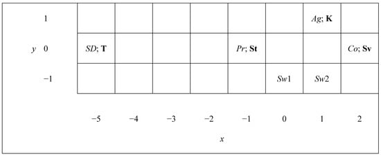
Figure 1.
Two-dimensional issue space for party groups and candidates. Traditional left-right dimension is on the x-axis; linguistic dimension (Swedish versus Finnish) is on the y-axis. Party groups: SD = Social Democrats; Pr = Progressives; Ag = Agrarians; Co = Conservatives; Sw1, Sw2 = blocs 1, 2 of Swedish People’s Party. Candidates: T = Tanner, St = Ståhlberg, K = Kallio, Sv = Svinhufvud.
Our weight ratios (Table 2) are taken as 2:1 except for the two Swedish blocs, which each receive 1:2 to reflect their strong concern for the linguistic dimension, and the Agrarians, with 1:1. As an illustration, the weighted squared distance between Sw1 and Svinhufvud is 1(0 − 2)2 + 2(−1 − 0)2 = 1·4 + 2·1 = 6. From low to high, the four values for Sw1 are 3 (Ståhlberg), 6 (Svinhufvud), 9 (Kallio), and 27 (Tanner), thus producing the preference ordering on the right side of Table 2.
All six of the preference orderings in Table 2—obtained using our (x, y) points and through the weight ratios : that differ by party group V—agree with the documented orderings in Table 1. They, thus, beget the same Condorcet cycle.
If for all six party groups : were set alike (to w1:w2) as either 2:1 or 1:1 (though not 1:2), one can show that no cycle would arise. See Appendix A.7 for details.
The 1931 Finnish presidential election provides a far-from-perfect illustration for our work. However, it does show how an election with a Condorcet cycle can be fitted by a model that has a two-dimensional issue space together with differential weights for the voters.
9. Summary
Different aspects of our work may be of significance or have interesting implications. Our work brings out some benefits of continuous (versus discrete) ideal-point distributions and infinite (versus finite) electorates. It calls attention to the topic, mostly neglected heretofore, of voters’ differential weightings of issues. The findings on the failure of symmetry to preclude cycles under differential weighting may be of some theoretical interest, and our approach to proofs in Section 3 for the case of equal weighting and an infinite electorate may have some pedagogical advantages over alternative methods.
We showed that, even under the stringent condition of radial symmetry (which we define for an infinite electorate), Condorcet cycles can occur if voters differ on their weightings of issues (though not if they do not differ). It is reasonable to hypothesize that this theoretical result has a real-world counterpart: that, in empirical settings (necessarily without radial symmetry), the absence of Condorcet winners stemming from Condorcet cycles will occur more often where voters weight the issues heterogeneously. Such a hypothesis might be examined. If it holds, the question may arise, in some cases, as to whether measures to try to lessen voters’ differences in issue weightings could (or should) be taken to try to reduce cycles and associated instability.
Funding
This research received no external funding.
Data Availability Statement
All data used in this paper are hypothetical and are shown in the paper itself.
Acknowledgments
The author thanks the three anonymous reviewers for their useful comments.
Conflicts of Interest
The author declares no conflict of interest.
Appendix A
Appendix A.1. Details for Examples 1.1 and 1.2
A voter V in the first half of the electorate has preferences as follows:
- V prefers A to B if xV < 2 [since ½(xA + xB) = ½(1 + 3) = 2],
- V prefers B to C if xV > −3,
- V prefers A to C if xV > −4,
- and conversely (e.g., V prefers B to A if xV > 2). The preferences of a voter V who is in the second half are:
- V prefers A to B if yV > 0 [since ½(yA + yB) = 0],
- V prefers B to C if yV < −1,
- V prefers A to C if yV > 6,
- and conversely.
Example 1.1.
The ideal points follow the uncorrelated bivariate normal distribution (means of 0, standard deviations equal to 10). Let Φ(•) denote the cumulative distribution function of the standard (univariate) normal distribution (with mean 0 and variance 1). Then, the proportion of the electorate
- that prefers A to B is [Φ(0.2) + 1 − Φ(0)]/2,
- >½ since Φ(0.2) > Φ(0);
- that prefers B to C is [1 − Φ(−0.3) + Φ(−0.1)]/2,
- >½ since Φ(−0.1) > Φ(−0.3); and
- that prefers A to C is [1 − Φ(−0.4) + 1 − Φ(0.6)]/2 = [Φ(0.4) + 1 − Φ(0.6)]/2,
- <½ since Φ(0.6) > Φ(0.4).
Thus A►B, B►C, and C►A.
Example 1.2.
The distribution of ideal points is uniform rather than bivariate normal. Then the proportion of the electorate
- that prefers A to B is = 55%;
- that prefers B to C is = 55%; and
- that prefers A to C is = 45%.
Thus A►B, B►C, and C►A with 55%-to-45% preference margins in all three cases.
Appendix A.2. Details for Example 2
Table A1 shows that the cycle A►B, B►C, C►A results. To illustrate the calculations, we consider the bottom of the table. The last two lines show that A►C for 69.4% and 30% of the halves of the electorate with 10:1 and 1:10 weight ratios, respectively. Thus C►A overall, by 50.3% to 49.7%.
For the last line, with a 1:10 weight ratio, (2) in the main text yields
or
as the applicable bisector of . This bisector intersects the line segment at (x, y) = (−4, 6), and crosses the left side of the square at y = 9, the right side at y = −1, and the y-axis at y = 4. Because the average ordinate of the bisector is y = 4, the proportion of the group that prefers A to C is = 30%.
20(x + 2y − 8) = 0,
Remark.
The same cycle of A►B, B►C, C►A also emerges if (at each point in the issue space) w1:w2 follows a continuous distribution over the range from (:, :) to (1:0, 0:1)—for instance, half (1 − u):u and half u:(1 − u) with u distributed according to the uniform (rectangular) distribution on the interval [0, 1].
Table A1.
Details demonstrating the existence of the Condorcet cycle.
Table A1.
Details demonstrating the existence of the Condorcet cycle.
| Candidate | Midpoint | Weight Ratio, w1:w2 | Value of | % of Electorate with G►H | ||||||||
|---|---|---|---|---|---|---|---|---|---|---|---|---|
| G at (xG, yG) | H at (xH, yH) | y When x = | x When y = | |||||||||
| −10 | 0 | 10 | −10 | 0 | 10 | Each Half | Both | |||||
| A, (1, 7) | B, (3, −7) | (2, 0) | 10:1 | 4(−10x + 7y + 20) = 0 | −5 | 2 | 9 | (2 − (−10))/20 = 60% | 55.07% | |||
| 1:10 | 4(−x + 70y + 2) = 0 | −6/35 | −1/35 | 4/35 | (10 − (−1/35))/20 = 50.14% | |||||||
| B, (3, −7) | C, (−9, 5) | (−3, −1) | 10:1 | 24(10x − y + 29) = 0 | −3.9 | −2.9 | −1.9 | (10 − (−2.9))/20 = 64.5% | 55.5% | |||
| 1:10 | 24(x − 10y − 7) = 0 | −1.7 | −0.7 | 0.3 | (−0.7 − (−10))/20 = 46.5% | |||||||
| A, (1, 7) | C, (−9, 5) | (−4, 6) | 10:1 | 4(50x + y + 194) = 0 | −3.68 | −3.88 | −4.08 | (10 − (−3.88))/20 = 69.4% | 49.7% | |||
| 1:10 | 20(x + 2y − 8) = 0 | 9 | 4 | −1 | (10 − 4)/20 = 30% | |||||||
Appendix A.3. Details for Examples 3.1 and 3.2
A voter V in the first half of the electorate has these preferences:
- V prefers A to B if xV < 2,
- V prefers B to C if xV > 6,
- V prefers A to C if xV < 1,
- and conversely. The preferences of a voter V in the second half are:
- V prefers A to B if yV > 8,
- V prefers B to C if yV > −1,
- V prefers A to C if yV > 0,
- and conversely.
Example 3.1.
For the uncorrelated bivariate normal distribution, the proportion of voters
- that prefers A to B is [Φ(0.2) + 1 − Φ(0.8)]/2,
- <½ since Φ(0.8) > Φ(0.2);
- that prefers B to C is [1 – Φ(0.6) + 1 − Φ(−0.1)]/2 = [1 − Φ(0.6) + Φ(0.1)]/2,
- <½ since Φ(0.6) > Φ(0.1); and
- that prefers A to C is [Φ(0.1) + 1 − Φ(0)]/2,
- >½ since Φ(0.1) > Φ(0).
Thus B►A, C►B, and A►C.
Example 3.2.
For the uniform distribution, the proportion of the electorate
- that prefers A to B is = 35%;
- that prefers B to C is = 37.5%; and
- that prefers A to C is = 52.5%.
Again, B►A, C►B, and A►C.
Appendix A.4. Details for Example 4
For the third group (the one with 88% of the voters):
The perpendicular bisector of the line segment intersects at (x, y) = (2, 8) and crosses the top of the square (y = 10) at x = 2.4, the bottom at x = −1.6, and the x-axis at x = 0.4. The proportion of the group that prefers A to B is thus = 52%.
The perpendicular bisector of crosses at (x, y) = (6, −1), the left side of the square (x = −10) at y = 1, the right side at y = −1.5, and the y-axis at y = −0.25. Thus, the proportion of the group that prefers B to C is = 51.25%.
The perpendicular bisector of crosses at (x, y) = (1, 0), the left side of the square at y = , the right side at y = 4, and the y-axis at y = . The proportion of the group that prefers A to C is, therefore, = 52.22%.
Within the third group, of course, no cycle exists: A►B, B►C, and A►C.
The proportions for the first two groups (35%, 37.5%, 52.5%) are the ones obtained for Example 3.2 in Appendix A.3 just above. Thus, across all three groups, the proportion of the electorate
- that prefers A to B is (0.12 × 35%) + (0.88 × 52%) = 49.96%;
- that prefers B to C is (0.12 × 37.5%) + (0.88 × 51.25%) = 49.6%; and
- that prefers A to C is (0.12 × 52.5%) + (0.88 × 52.22%) = 52.26%.
Therefore, for the entire electorate, the result is B►A, C►B, and A►C.
Appendix A.5. Details for Example 5
Table A2 (top part) establishes the Condorcet cycle when voters’ weightings are disparate. The bottom part of the table confirms that no cycle exists when all voters are alike in their weightings of the issues.
Table A2.
Weighted a squared distance from each voter to each candidate, and preference rankings and matchups.
Table A2.
Weighted a squared distance from each voter to each candidate, and preference rankings and matchups.
| Weighted a Squared Distance | Preference Matchups | ||||||||||
|---|---|---|---|---|---|---|---|---|---|---|---|
| Weight Ratio | Candidate | Ranking | A vs. B | B vs. C | C vs. A | ||||||
| Voter(s) | A, (1, 7) | B, (3, −7) | C, (−9, 5) | A | B | B | C | C | A | ||
| V1, (−6, 2) | 7:1 | 7∙49 + 25 = 368 | 7∙81 + 81 = 648 | 7∙9 + 9 = 72 | C A B | 1 | 0 | 0 | 1 | 1 | 0 |
| V5, (−6, 2) | 1:7 | 49 + 7∙25 = 224 | 81∙7 + 81 = 648 | 9 + 7∙9 = 72 | C A B | 1 | 0 | 0 | 1 | 1 | 0 |
| V2, (6, 2) | 7:1 | 7∙25 + 25 = 200 | 7∙9 + 81 = 144 | 7∙225 + 9 = 1584 | B A C | 0 | 1 | 1 | 0 | 0 | 1 |
| V6, (6, 2) | 1:7 | 25 + 7∙25 = 200 | 9 + 7∙81 = 576 | 225 + 7∙9 = 288 | A C B | 1 | 0 | 0 | 1 | 0 | 1 |
| V3, (−6, −2) | 7:1 | 7∙49 + 81 = 424 | 7∙81 + 25 = 592 | 7∙9 + 49 = 112 | C A B | 1 | 0 | 0 | 1 | 1 | 0 |
| V7, (−6, −2) | 1:7 | 49 + 7∙81 = 616 | 81 + 7∙25 = 256 | 9 + 7∙49 = 352 | B C A | 0 | 1 | 1 | 0 | 1 | 0 |
| V4, (6, −2) | 7:1 | 7∙25 + 81 = 256 | 7∙9 + 25 = 88 | 7∙225 + 49 = 1624 | B A C | 0 | 1 | 1 | 0 | 0 | 1 |
| V8, (6, −2) | 1:7 | 25 + 7∙81 = 592 | 9 + 7∙25 = 184 | 225 + 7∙49 = 568 | B C A | 0 | 1 | 1 | 0 | 1 | 0 |
| V9, (0, 0) | 1:1 | 1 + 49 = 50 | 9 + 49 = 58 | 81 + 25 = 106 | A B C | 1 | 0 | 1 | 0 | 0 | 1 |
| All | 5 | 4 | 5 | 4 | 5 | 4 | |||||
| V1 and V5 | 1:1 | 49 + 25 = 74 | 81 + 81 = 162 | 9 + 9 = 18 | C A B | 2 | 0 | 0 | 2 | 2 | 0 |
| V2 and V6 | 1:1 | 25 + 25 = 50 | 9 + 81 = 90 | 225 + 9 = 234 | A B C | 2 | 0 | 2 | 0 | 0 | 2 |
| V3 and V7 | 1:1 | 49 + 81 = 130 | 81 + 25 = 106 | 9 + 49 = 58 | C B A | 0 | 2 | 0 | 2 | 2 | 0 |
| V4 and V8 | 1:1 | 25 + 81 = 106 | 9 + 25 = 34 | 225 + 49 = 274 | B A C | 0 | 2 | 2 | 0 | 0 | 2 |
| V9 | 1:1 | 1 + 49 = 50 | 9 + 49 = 58 | 81 + 25 = 106 | A B C | 1 | 0 | 1 | 0 | 0 | 1 |
| All | 5 | 4 | 5 | 4 | 4 | 5 | |||||
a Squared distances at the bottom of the table are unweighted.
Appendix A.6. Details for Example 6
Table A3 (top part) establishes the Condorcet cycle when voters’ weightings are disparate. The bottom part of the table confirms that no cycle exists when all voters are alike in their weightings of the issues.
Table A3.
Weighted a squared distance from each voter to each candidate, and preference rankings and matchups.
Table A3.
Weighted a squared distance from each voter to each candidate, and preference rankings and matchups.
| Weighted a Squared Distance | Preference Matchups | ||||||||||
|---|---|---|---|---|---|---|---|---|---|---|---|
| Weight Ratio | Candidate | Ranking | A vs. B | B vs. C | C vs. A | ||||||
| Voter | A, (1, 7) | B, (3, −7) | C, (−9, 5) | A | B | B | C | C | A | ||
| V5, (−6, 2) | 1:7 | 49 + 7∙25 = 224 | 81∙7 + 81 = 648 | 9 + 7∙9 = 72 | C A B | 1 | 0 | 0 | 1 | 1 | 0 |
| V2, (6, 2) | 7:1 | 7∙25 + 25 = 200 | 7∙9 + 81 = 144 | 7∙225 + 9 = 1584 | B A C | 0 | 1 | 1 | 0 | 0 | 1 |
| V3, (−6, −2) | 7:1 | 7∙49 + 81 = 424 | 7∙81 + 25 = 592 | 7∙9 + 49 = 112 | C A B | 1 | 0 | 0 | 1 | 1 | 0 |
| V8, (6, −2) | 1:7 | 25 + 7∙81 = 592 | 9 + 7∙25 = 184 | 225 + 7∙49 = 568 | B C A | 0 | 1 | 1 | 0 | 1 | 0 |
| V9, (0, 0) | 1:1 | 1 + 49 = 50 | 9 + 49 = 58 | 81 + 25 = 106 | A B C | 1 | 0 | 1 | 0 | 0 | 1 |
| All | 3 | 2 | 3 | 2 | 3 | 2 | |||||
| V5 | 1:1 | 49 + 25 = 74 | 81 + 81 = 162 | 9 + 9 = 18 | C A B | 1 | 0 | 0 | 1 | 1 | 0 |
| V2 | 1:1 | 25 + 25 = 50 | 9 + 81 = 90 | 225 + 9 = 234 | A B C | 1 | 0 | 1 | 0 | 0 | 1 |
| V3 | 1:1 | 49 + 81 = 130 | 81 + 25 = 106 | 9 + 49 = 58 | C B A | 0 | 1 | 0 | 1 | 1 | 0 |
| V8 | 1:1 | 25 + 81 = 106 | 9 + 25 = 34 | 225 + 49 = 274 | B A C | 0 | 1 | 1 | 0 | 0 | 1 |
| V9 | 1:1 | 1 + 49 = 50 | 9 + 49 = 58 | 81 + 25 = 106 | A B C | 1 | 0 | 1 | 0 | 0 | 1 |
| All | 3 | 2 | 3 | 2 | 2 | 3 | |||||
a Squared distances at the bottom of the table are unweighted.
Appendix A.7. Details for Statement about 1931 Finnish Election
Parts (a), (b), and (c) of Table A4, for respective common weight ratios for all six party groups of 2:1, 1:1, and 1:2, establish that a Condorcet cycle still occurs only in the third case and not in the first two.
Table A4.
Weighted squared distance from each party group to each candidate, plus preference rankings and matchups.
Table A4.
Weighted squared distance from each party group to each candidate, plus preference rankings and matchups.
| (a) Weight ratio is common at 2:1 within each party group and across all party groups. | |||||||||||||
|---|---|---|---|---|---|---|---|---|---|---|---|---|---|
| Weighted Squared Distance | |||||||||||||
| Va | Spatial Location of V | Candidate, b G, and His Spatial Location, PG: (xG, yG) | Preference Ranking b | No. of Electors | Head-to-Head Preference Matchups b | ||||||||
| T | St | K | Sv | St vs. K | K vs. Sv | Sv vs. St | |||||||
| (−5, 0) | (−1, 0) | (1, 1) | (2, 0) | St | K | K | Sv | Sv | St | ||||
| SD | (−5, 0) | 0 | 32 | 73 | 98 | T St K Sv | 90 | 90 | 0 | 90 | 0 | 0 | 90 |
| Pr | (−1, 0) | 32 | 0 | 9 | 18 | St K Sv T | 52 | 52 | 0 | 52 | 0 | 0 | 52 |
| Ag | (1, 1) | 73 | 9 | 0 | 3 | K Sv St T | 69 | 0 | 69 | 69 | 0 | 69 | 0 |
| Co | (2, 0) | 98 | 18 | 3 | 0 | Sv K St T | 64 | 0 | 64 | 0 | 64 | 64 | 0 |
| Sw1 | (0, −1) | 51 | 3 | 6 | 9 | St K Sv T | 7 | 7 | 0 | 7 | 0 | 0 | 7 |
| Sw2 | (1, −1) | 73 | 9 | 4 | 3 | Sv K St T | 18 | 0 | 18 | 0 | 18 | 18 | 0 |
| All | 300 | 149 | 151 | 218 | 82 | 151 | 149 | ||||||
| (b) Weight ratio is common at 1:1 within each party group and across all party groups. | |||||||||||||
| Weighted Squared Distance | |||||||||||||
| Va | Spatial Location of V | Candidate, b G, and His Spatial Location, PG: (xG, yG) | Preference Ranking b | No. of Electors | Head-to-Head Preference Matchups b | ||||||||
| T | St | K | Sv | St vs. K | K vs. Sv | Sv vs. St | |||||||
| (−5, 0) | (−1, 0) | (1, 1) | (2, 0) | St | K | K | Sv | Sv | St | ||||
| SD | (−5, 0) | 0 | 16 | 37 | 49 | T St K Sv | 90 | 90 | 0 | 90 | 0 | 0 | 90 |
| Pr | (−1, 0) | 16 | 0 | 5 | 9 | St K Sv T | 52 | 52 | 0 | 52 | 0 | 0 | 52 |
| Ag | (1, 1) | 37 | 5 | 0 | 2 | K Sv St T | 69 | 0 | 69 | 69 | 0 | 69 | 0 |
| Co | (2, 0) | 49 | 9 | 2 | 0 | Sv K St T | 64 | 0 | 64 | 0 | 64 | 64 | 0 |
| Sw1 | (0, −1) | 26 | 2 | 5 | 5 | St K = Sv T | 7 | 7 | 0 | 3½ | 3½ | 0 | 7 |
| Sw2 | (1, −1) | 37 | 5 | 4 | 2 | Sv K St T | 18 | 0 | 18 | 0 | 18 | 18 | 0 |
| All | 300 | 149 | 151 | 214½ | 85½ | 151 | 149 | ||||||
| (c) Weight ratio is common at 1:2 within each party group and across all party groups. | |||||||||||||
| Weighted Squared Distance | |||||||||||||
| Va | Spatial Location of V | Candidate, b G, and His Spatial Location, PG: (xG, yG) | Preference Ranking b | No. of Electors | Head-to-Head Preference Matchups b | ||||||||
| T | St | K | Sv | St vs. K | K vs. Sv | Sv vs. St | |||||||
| (−5, 0) | (−1, 0) | (1, 1) | (2, 0) | St | K | K | Sv | Sv | St | ||||
| SD | (−5, 0) | 0 | 16 | 38 | 49 | T St K Sv | 90 | 90 | 0 | 90 | 0 | 0 | 90 |
| Pr | (−1, 0) | 16 | 0 | 6 | 9 | St K Sv T | 52 | 52 | 0 | 52 | 0 | 0 | 52 |
| Ag | (1, 1) | 38 | 6 | 0 | 3 | K Sv St T | 69 | 0 | 69 | 69 | 0 | 69 | 0 |
| Co | (2, 0) | 49 | 9 | 3 | 0 | Sv K St T | 64 | 0 | 64 | 0 | 64 | 64 | 0 |
| Sw1 | (0, −1) | 27 | 3 | 9 | 6 | St Sv K T | 7 | 7 | 0 | 0 | 7 | 0 | 7 |
| Sw2 | (1, −1) | 38 | 6 | 8 | 3 | Sv St K T | 18 | 18 | 0 | 0 | 18 | 18 | 0 |
| All | 300 | 167 | 133 | 211 | 89 | 151 | 149 | ||||||
a V is for party group: SD = Social Democrats; Pr = Progressives; Ag = Agrarians; Co = Conservatives; Sw1, Sw2 = blocs 1, 2 of Swedish People’s Party. b Candidates: T = Tanner, St = Ståhlberg, K = Kallio, Sv = Svinhufvud.
References
- Abramson, Paul R., John H. Aldrich, and David W. Rohde. 2002. Change and Continuity in the 2000 Elections. Washington, DC: CQ Press. [Google Scholar]
- Adams, James. 1997. Condorcet efficiency and the behavioral model of the vote. The Journal of Politics 59: 1252–63. [Google Scholar] [CrossRef]
- Adams, James F., and Ernest W. Adams. 2000. The geometry of voting cycles. Journal of Theoretical Politics 12: 131–53. [Google Scholar] [CrossRef]
- Caplin, Andrew, and Barry Nalebuff. 1988. On 64% majority rule. Econometrica 56: 787–814. [Google Scholar] [CrossRef][Green Version]
- Dasgupta, Partha, and Eric Maskin. 2004. The fairest vote of all. Scientific American 290: 92–97. [Google Scholar] [CrossRef]
- Davis, Otto A., and Melvin J. Hinich. 1968. On the power and importance of the mean preference in a mathematical model of democratic choice. Public Choice 5: 59–72. [Google Scholar] [CrossRef]
- Davis, Otto A., Melvin J. Hinich, and Peter C. Ordeshook. 1970. An expository development of a mathematical model of the electoral process. American Political Science Review 64: 426–48. [Google Scholar] [CrossRef]
- Davis, Otto A., Morris H. DeGroot, and Melvin J. Hinich. 1972. Social preference orderings and majority rule. Econometrica 40: 147–57. [Google Scholar] [CrossRef]
- Erikson, Robert S., and David W. Romero. 1990. Candidate equilibrium and the behavioral model of the vote. American Political Science Review 84: 1103–26. [Google Scholar] [CrossRef]
- FairVote. 2019. Democratic Primary 2020 Interactive—20 Candidates. Available online: https://www.fairvote.org/interact_with_the_data?utm_campaign=yougov_poll&utm_medium=email&utm_source=fairvote (accessed on 25 September 2019).
- FairVote. 2020. Report on FairVote/SurveyUSA National Poll of the 2020 Democratic Presidential Field, Table 2, “Head-to-Head Matchups”. Available online: https://fairvote.app.box.com/s/8syue8jxdikiueknwaoedpar9q9w6roj (accessed on 22 March 2020).
- Feld, Scott L., and Bernard Grofman. 1987. Necessary and sufficient conditions for a majority winner in n-dimensional spatial voting games: An intuitive geometric approach. American Journal of Political Science 31: 709–28. [Google Scholar] [CrossRef]
- Feld, Scott L., Samuel Merrill, III, and Bernard Grofman. 2014. Modeling the effects of changing issue salience in two-party competition. Public Choice 158: 465–82. [Google Scholar] [CrossRef]
- Gehrlein, William V. 2006. Condorcet’s Paradox. Berlin: Springer. [Google Scholar]
- Hinich, Melvin J., and Walker Pollard. 1981. A new approach to the spatial theory of electoral competition. American Journal of Political Science 25: 323–41. [Google Scholar] [CrossRef]
- Hoyer, R. W., and Lawrence S. Mayer. 1974. Comparing strategies in a spatial model of electoral competition. American Journal of Political Science 18: 501–23. [Google Scholar] [CrossRef]
- Hoyer, Robert W., and Lawrence S. Mayer. 1975. Social preference orderings under majority rule. Econometrica 43: 803–6. [Google Scholar] [CrossRef]
- Laatu, Juho, and Warren D. Smith. 2009. The Rank-Order Votes in the 2009 Burlington Mayoral Election. Available online: https://rangevoting.org/JLburl09.txt (accessed on 26 September 2019).
- Lagerspetz, Eerik. 2016. Social Choice and Democratic Values. Cham: Springer. [Google Scholar]
- Maskin, Eric, and Amartya Sen. 2018. Maine tries a better way to vote. New York Times, June 11, A21. [Google Scholar]
- Merrill, Samuel, III. 1988. Making Multicandidate Elections More Democratic. Princeton: Princeton University Press. [Google Scholar]
- Miller, Nicholas R. 2015. The spatial model of social choice and voting. In Handbook of Social Choice and Voting. Edited by Jac C. Heckelman and Nicholas R. Miller. Cheltenham: Edward Elgar Publishing, pp. 163–81. [Google Scholar]
- Niemi, Richard G., and Larry M. Bartels. 1985. New measures of issue salience: An evaluation. The Journal of Politics 47: 1212–20. [Google Scholar] [CrossRef]
- Olson, Brian. 2009. IRV Failure in the Real World. Available online: http://bolson.org/~bolson/2009/20090303_burlington_vt_mayor.html (accessed on 26 September 2019).
- Plott, Charles R. 1967. A notion of equilibrium and its possibility under majority rule. The American Economic Review 57: 787–806. [Google Scholar]
- Polk, Jonathan, Jan Rovny, Ryan Bakker, Erica Edwards, Liesbet Hooghe, Seth Jolly, Jelle Koedam, Filip Kostelka, Gary Marks, Gijs Schumacher, and et al. 2017. Explaining the salience of anti-elitism and reducing political corruption for political parties in Europe with the 2014 Chapel Hill Expert Survey data. Research & Politics 4. Januaru–March. [Google Scholar] [CrossRef]
- Potthoff, Richard F. 1970. The problem of the three-way election. In Essays in Probability and Statistics. Edited by Raj Chandra Bose, Indra M. Chakravarti, Prasanta Chandra Mahalanobis, Calyampudi Radhakrishna Rao and Kempton J. C. Smith. Chapel Hill: University of North Carolina Press, pp. 603–20. [Google Scholar]
- Rabinowitz, George, James W. Prothro, and William Jacoby. 1982. Salience as a factor in the impact of issues on candidate evaluation. The Journal of Politics 44: 41–63. [Google Scholar] [CrossRef]
- Regenwetter, Michel, Bernard Grofman, A. A. J. Marley, and Ilia Tsetlin. 2006. Behavioral Social Choice: Probabilistic Models, Statistical Inference, and Applications. Cambridge: Cambridge University Press. [Google Scholar]
- Rivers, Douglas. 1988. Heterogeneity in models of electoral choice. American Journal of Political Science 32: 737–57. [Google Scholar] [CrossRef]
- Saari, Donald G. 1995. Basic Geometry of Voting. Berlin: Springer. [Google Scholar]
- Saari, Donald G. 1997. The generic existence of a core for q-values. Economic Theory 9: 219–60. [Google Scholar]
- Schofield, Norman. 2008. The Spatial Model of Politics. London: Routledge. [Google Scholar]
- Simpson, Paul B. 1969. On defining areas of voter choice: Professor Tullock on stable voting. The Quarterly Journal of Economics 83: 478–90. [Google Scholar] [CrossRef]
- Tullock, Gordon. 1967. The general irrelevance of the general impossibility theorem. The Quarterly Journal of Economics 81: 256–70. [Google Scholar] [CrossRef]
- Van Deemen, Adrian. 2014. On the empirical relevance of Condorcet’s paradox. Public Choice 158: 311–30. [Google Scholar] [CrossRef]

Publisher’s Note: MDPI stays neutral with regard to jurisdictional claims in published maps and institutional affiliations. |
© 2022 by the author. Licensee MDPI, Basel, Switzerland. This article is an open access article distributed under the terms and conditions of the Creative Commons Attribution (CC BY) license (https://creativecommons.org/licenses/by/4.0/).