Abstract
Several fiscal policy strategies have been implemented in South Africa since 1994, starting from the Reconstruction and Development Programme (RDP), Growth Employment and Redistribution (GEAR), Broad-Black Economic Empowerment strategy (BEE), AsgiSA (Accelerated and shared growth initiative for South Africa), and the New Growth Path framework (NGP) with the aim of boosting economic growth. However, the rate of economic growth in the country over the years is not convincing. It is also important to note that poverty still remains prevalent and persistent, predominantly in the poverty-stricken areas of provinces such as Eastern Cape, Limpopo, North West, and Mpumalanga. In light of this, the main aim of the study was to examine the effect of fiscal policy instruments on economic growth in South Africa for the period from 1988 to 2018, utilising the autoregressive distributed lag model, mainly due to the order of integration of the variables. Empirical results revealed that there is a positive relationship between fiscal policy instruments (public sector expenditure, public consumption spending, and taxation) and economic growth. Based on the findings, the study recommends that the government should distinguish between productive and unproductive spending and increase spending on productive sectors. The implication of these findings is that South Africa’s economy is likely to perform better if more resources are diverted from government consumption to investment spending.
1. Introduction and Background of Study
The role of fiscal policy in the economy is well-documented in the literature by researchers such as Hlongwane et al. (2018), Heitger (2018), Ahmad et al. (2020), Nuru and Gereziher (2021), and Pamba (2021). The available studies in this area highlight that fiscal policy can influence economic growth through both the macroeconomic and microeconomic channels (International Monetary Fund 2011). At the macroeconomic level, Kim et al. (2021) argued that fiscal sustainability is the cornerstone of macroeconomic stability. This is also important for economic growth as a country that has high levels of deficit and is more likely to experience macroeconomic instability, which may also deter private investment. In this paper, the authors show that at the macroeconomic level, taxes and government spending can influence firm operations, as well as research and development (R&D). In addition, public expenditure goes a long way in contributing towards education and human capital formation, as well as healthcare.
The empirical literature anchored in the classical view and Keynesian view presents mixed results on the relationship between fiscal policy and economic growth, with researchers such as Nourzad and Vrieze (2017), Heitger (2018), and Hauptmeier et al. (2018) supporting the classical view that an increase in government expenditure and decrease in tax would increase demand for money. Assuming that the money supply is fixed by the Reserve Bank, this would increase the interest rate and crowd out capital accumulation (private investment would decline). A fall in private investment could have a multiple negative effect on output (offset the Keynesian multiple effect) and hinder economic growth. On the other hand, researchers Adegbite and Owulabi (2015), Ocran (2011), Akanbi (2013) and Djelloul et al. (2014) supported the Keynesian view that the government should provide public goods, maintain law and order, increase productive investment and research and development, and increase human capital development to stimulate short-term and long-term economic growth.
In the case of South Africa, the government adopted an expansionary fiscal policy after 1994 as a recovery and consolidation technique. Government spending comprises primarily two aspects, government investment spending and government consumption spending. Akanbi (2013) argued that government consumption expenditure forms nearly thirty percent (30%) of aggregate domestic demand and tax revenue finance nearly 95% of government consumption expenditure, which means the impact of fiscal policy in stabilising the South African economy could not be underestimated.
Of the different government policies implemented by the country in 1996, the South African government implemented the GEAR strategy as a substitute to the RDP policy (Ocran 2011). The main objective of the GEAR strategy was to enhance the economic growth rate and redistribute income in the economy. The GEAR policy recognised higher economic growth (Bhorat and Oosthuizen 2004). Recently, the government implemented policies such as Skills Development programs, the Black Economic Empowerment Act, and the availability of social grants to those who qualify, in order to create employment and redistribute income, as well as achieve high levels of economic growth. Additionally, looking at government expenditure as a percentage of GDP, in 2006, it stood at 20%. This increased to 29.91% in 2016, and in 2020, it rose to 35.98%. Though these increases may be linked to COVID-19, it is important to observe that the years prior to 2020, the country had breached the 30% mark.
However, it is interesting to note that despite all the increase in government expenditure, economic growth still remains very low. According to South African Reserve Bank (2016), GDP in South Africa rose at an average of 3.1% for the period between 1994–2016. The country encountered high growth between 2004 and 2008, and growth in this period averaged 4.9%, while 5.6% was attained in 2006 and 2007. The global financial crisis, which began in 2008, led to the economy slipping into a domestic recession in 2009, with a contraction in GDP of 1.5 percent. The recession wiped out the gains experienced by the economy in the previous years. During the period from 2010 to 2016, GDP growth was slow, with an average growth of 2.8 percent (Parkin et al. 2012). This has become worse off with the COVID-19 pandemic.
In addition, a study by Mo (2007) showed that “government services provide political, social and legal rules for production, exchange and distribution that can promote market exchanges and innovations. Some government services are therefore essential for enhancing growth in productivity and capital. However, government can just create jobs for itself and produce services that are neither directly or indirectly productive. The larger the government expenditures, the smaller the resources available in private markets will be. The incentive for innovation, enterprising activities and investment will be reduced”. This becomes important for a country such as South Africa, where government expenditure has been on the rise, and at the same time, economic growth is sluggish.
The study, therefore, sought to examine the impact of fiscal policy on economic growth in South Africa. Empirically, in South Africa, a number of scholars, for example, Nourzad and Vrieze (2017), Heitger (2018), and Hauptmeier et al. (2018), used panel data and structural vector autoregression (SVAR) to examine the macroeconomic impact of fiscal policy, fiscal policy sustainability, and the effect of its instruments on the GDP growth rate. The study expanded on the debate between the variables of interest, using a time series approach. Odhiambo (2009) indicated that country-specific studies may provide robust results as opposed to cross-sectional studies. The author further highlighted that panel or cross-sectional studies may impose homogeneity on coefficients, which, in reality, may vary across countries due to a number of factors, such as institutional setups, domestic economic policy, and political and economic structures. Furthermore, the study utilised the ARDL model, which is able to deal with integrated data of different orders. The results revealed that there is a positive relationship between fiscal policy instruments (public sector expenditure, public consumption spending, and taxation) and economic growth.
This paper is divided into four major sections. Following the introduction, Section 2 focuses on literature review and theoretical framework, Section 3 discusses the methodology, and results are interpreted in Section 4. Section 5 concludes the study, as it provides policy recommendations and highlights some limitations encountered in the study.
2. Literature Review and Theoretical Framework
Theories used to analyse the impact of fiscal policy on economic growth in this study include the Keynesian view on fiscal policy, the Harrod–Domar growth model, neoclassical views, endogenous growth models, and the Ricardian equivalence theory. Keynesians believe that government intervention is the key to resolve economic problems (Barro 1999). Keynes declared that when an economy is in a state of high unemployment and low economic growth, it should adopt an expansionary fiscal policy by means of increased government expenditure and/or a cut in taxes to expand the economy and boost economic activities. However, the Harrod–Domar growth model suggests that a fiscal policy that induces the savings rate could promote growth. Nevertheless, the fact that the capital output ratios are assumed to be given and technology does not influence growth, limits its applicability to explain real situations. In addition, the Keynesian view is contradicted by the neoclassical view, which argues that government intervention in the economy has minimal effects on economic growth and the distribution of income.
According to the neoclassical theory, an expansionary fiscal policy or running a fiscal deficit may retard growth. Neoclassical economists contend that the Keynesian theory overlooks the secondary effects of fiscal policy. Diamond (1965) reaffirmed the neoclassical view against an expansionary fiscal policy and budget deficits. The argument was that an expansionary fiscal policy might raise interest rates, which would have a crowding-out effect on private capital accumulation. The neoclassical view is supported by various researchers, which include Auerbach and Kotlikoff (1987), Diamond (1965), and Taylor (2009), among others. Their argument was based on the notion that running a budget deficit would always cause the crowding-out effect that is postulated by the standard ISLM analysis.
Endogenous growth models postulate to address neoclassical shortcomings (Romer 1986). These models analyse growth, using changes in technology and production factors. DeLong and Summers (1991) argued that the endogenous growth theory explains that any fiscal policy that enhances savings and investment, including investment in human capital, research and development, as well technological innovation, would lead to increased growth. Under the endogenous models, knowhow is a very important factor for enhancing savings and investment to boost economic growth.
In addition, the more recent theory that differs from the Keynesian theory is the neo-Keynesian theory. According to Christiano et al. (2005), neo-Keynesians do not believe that market equilibrium will be achieved naturally. This means the invisible hand could not work in this model, and full employment cannot be achieved automatically. The neo-Keynesian believed that it is only the government, through its policies, that can ensure full employment (Perotti 2007).
David Ricardo’s equivalence theory postulates that running a fiscal deficit or expansionary fiscal policy does not have a significant influence on aggregate demand, investment, and the GDP growth rate (Dalyop 2019). The Ricardian equivalence theory argues that a fiscal deficit cannot stimulate aggregate demand, and thus cannot increase economic growth, and the reason is that, when an expansionary fiscal policy is implemented, households tend not to consume more, but they save in expectation of increased tax burdens in the future (Corden 1991).
Several attempts have been made by numerous researchers in different economies to examine the relationship between fiscal policy, economic growth, and income distribution using different methods. Researchers such as Adegbite and Owulabi (2015), Ocran (2011), Akanbi (2013) and Djelloul et al. (2014) established a positive relationship between fiscal policy and economic growth. They supported the Keynesian view that government should provide public goods, maintain law and order, increase productive investment and research and development, and increase human capital development to stimulate short-term and long-term economic growth.
On the other hand, researchers such as Nourzad and Vrieze (2017), Heitger (2018), and Hauptmeier et al. (2018) established a negative relationship between fiscal policy and economic growth, supporting the classical view that an increase in government expenditure and decrease in tax would increase demand for money. Assuming that the money supply is fixed by the Reserve Bank, this would increase the interest rate and crowd out capital accumulation (private investment would decline). A fall in private investment could have a multiple negative effect on output (offset the Keynesian multiple effect) and hinder economic growth.
Another strand of literature insinuates that some fiscal policy instruments have a neutral impact on economic growth; for instance, the Djelloul et al. (2014) and M’Amanja and Morrissey (2015) studies indicated that non-distortionary tax revenue and unproductive spending are neutral to growth, as predicted. Their studies also found productive government spending to have a significant negative relationship with growth in the short-run, and no evidence was found on the effects of distortionary taxes on economic growth. However, the study concluded that, in the long-run, government investment could improve economic growth. Lastly, Ocran (2011) used the vector regressive model to investigate how the fiscal policy instruments impact economic growth in South Africa, and the study concluded that budget deficit has no significant influence on output growth.
Given the contradictory results observed in the above stated studies, it is imperative to examine the extent to which fiscal policy impacts economic growth in the South African context. The current study disaggregated the fiscal policy variables so as to analyse their different impacts on economic growth. The focus was on establishing whether public sector investment and government consumption have the same or differing effects. The literature suggests that expenditure that is not channelled towards investment does not have a significant impact on economic growth. This is of great importance considering the expenditure that is channelled towards consumption expenditure in the country.
3. Methodology and Data
3.1. Theoretical Framework and Model Specification
The study adopted the fiscal policy theory propounded by Musgrave (1959). Musgrave’s theory postulates that macroeconomic factors such as economic growth, income inequality, employment, inflation, and balance of payments stability can be influenced by changes in fiscal and monetary policy instruments, such as taxes, government expenditure, exchange rates, rate of interest, capital formation, and so on. Therefore, the model can be as follows:
Yi = f(x1, x2, x3………..xj)
= economic growth, income inequality, employment, inflation, and balance of payments stability. = policy instrument (taxes, government expenditure, exchange rates, interest rates, and capital flows (i.e., as a variable influencing balance of payments)). The model above shows us that policy instruments can efficiently influence the macroeconomic variables. If, for instance, the government wants to influence the macroeconomic variable (income distribution), it must work on the policy tool first (expenditure and/or taxes). If a slight adjustment of the policy instrument has a multiple effect on the dependent variable, Musgrave (1959) asserts that the policy tool will be regarded as efficient to the dependent variable.
Based on the theoretical considerations discussed above, the study modified the equation by Daniel M’Amanja and Morrissey (2015), as formally specified below.
where GDP_RATEt = the real gross domestic product rate in year t, PSIt is public sector investment in year t, GCEXt is government consumption expenditure in year t, TRt is tax revenue in year t, DPRIt is domestic private investment in year t, PIt is portfolio investment in year t, INFLt is inflation rate in year t, TOT_INDXt is the terms of trade index in year t, REERt is real effective exchange rate in year t, and FDIt is foreign direct investment in year t.
The study introduced a logarithm to the model, assuming a constant, α; coefficients of independent variables, β1–β7; and an error term t, and the model became:
Logarithms were introduced, since we were dealing with a growth function or changes in the variables; the log expression, which is usually followed, was appropriate for this purpose, since it virtually refers to percentage changes in the variables.
3.2. Economic Variables Definitions and Their A Priori Expectations
Gross domestic product: This is the real GDP, which refers to a macroeconomic measure of value of output produced within the boundaries of an economy, and it is adjusted for inflation or deflation. The GDP was changed to logarithms. Change in GDP is a measure of economic growth. This dependent variable needs to be tested. Public investment spending (excluding investment in education) measures the total expenditure by the government on public services, and it is expected to positively influence economic growth through the multiplier effect, as supported by Ramey (2011). Government consumption expenditure refers to all the expenditure by the government that does not bring direct income to the state, for example, expenditure on social grants, health, education, and fighting crime, among others (Treasury 2017).
A positive result was expected, as supported by Fisher (1993), who argued that consumption expenditure is an injection to the economy that increases national income. Total revenue is the revenue that comes mainly from taxes, which includes company tax, personal income tax, and value-added tax (VAT), customs, and excise. The study expected a positive sign between total revenue collected and economic growth (Karagianni and Pempetzogloub 2012).
Domestic private investment can be defined as the amount of money that domestic firms invest within their own economy and is expected to be positive. Uremadu (2012), as well as Adegbite and Owulabi (2015), argued that direct private investment is an injection to the economy; therefore, it has a greater multiplier effect on national output. Portfolio investment refers to all assets that an investor holds, such as property titles, bonds, stocks, options, and other securities. A positive relationship was expected between portfolio investment and economic growth, as argued by Perotti (2007). Portfolio investment brings a huge increase in capital inflows that boost production and enhance economic growth (Perotti 2007). Inflation measures the consumer price index and is based on the change from the previous year. Ramey (2011) argued that continued increase in general price level can affect the wealth of the citizens, which will, in turn, affect saving and investment; therefore, a negative or positive sign can be expected.
Terms of trade index is the comparative value of exports expressed in terms of imports value. Shahbaz et al. (2010) concluded that an increase in TOT indicates an increase export supply, a structural change in exports that influences domestic output and increases productivity, reduces unemployment, and increases the GDP rate. Therefore, the study expected a positive sign between the TOT index and GDP rate. Real effective exchange rates refer to the weighted average index of an economy’s currency compared to the weighted index of another economy’s currency. The variable was expected to positively affect economic growth, and this can be supported by Rodrik (2007), who argued that the depreciation of currency promotes exports, and that would promote economic growth. Foreign direct investment (FDI) is used as a proxy of financial openness, and the study posited it to be a positive sign. According to Duncan and Peter (2008), the liberalization of financial markets can bring enormous amounts of investments from the foreign sector, for example, FDI, and this can lead to an increase in national output through the multiplier effect.
3.3. Data Sources
The dataset is for 30 years, the period from 1988 to 2018, and is on quarterly bases. The data are from the Department of Trade, the Reserve Bank of South Africa online data download facility, the World Bank national accounts data online, the Quantec Easy Data, and the South Africa Statistics online.
3.4. Estimation Technique
This study examined the impact of fiscal policy on economic growth using the autoregressive distributed lag (ARDL) method. Before starting the ARDL steps, studying the time series properties of all variables was necessary. Formally, in addition to the informal testing, which involved graphical analysis, the study employed the augmented Dickey–Fuller model (ADF) and Phillips–Perron method to determine the unit root of the issue. It is more efficient to use this ARDL approach on long-run parameter estimates, as well as being more heterogeneous, as it allows the estimated standard errors to be unbiased. A second advantage of ARDL over other approaches is that it fixes both the endogenous regressors and autocorrelation issues simultaneously, as well as the fact that it can be applied even when the variables have different orders, unlike other approaches, such as Johansen, which require identical variables (Pesaran and Pesaran 1997).
The ARDL estimates and t-tests sizes were assumed to be reliable and effective, compared to other approaches. Lastly, the approach took preference due to the exceptional estimates of power being found reliable and more efficient in small samples compared to that of the Johansen technique. The first step of the ARDL process is to establish the maximum lags to determine the co-integration of variables; the study employed the bounds F-test. The F-test being higher than at least one of I1 bound values confirms co-integration. If the computed F-value is greater than l1 bound value at all levels (1%, 5%, and 10%), it reveals that the variables are co-integrated; therefore, short-run and long-run tests are conducted.
Once the long-run relationship is established, long-run and short run coefficients of the proposed ARDL models are then estimated. The long-run ARDL equilibrium of the model is as follows:
The Akaike information criterion (AIC) was used to determine the lag length which was used to estimate the ARDL model. Using time series data for the study, Perman (1991) proposed that the maximum lag length is 2. The short-run elasticities can be derived by formulating the error correction model as follows:
In addition, diagnostic tests are conducted after the long-run and short-run tests. Diagnostic tests are employed to check the fitness of the model, particularly by analysing misspecification, serial correlation, and heteroskedasticity linked to the specified model (Brooks 2008). A CUSUM of squares test and CUSUM test are the last steps of the ARDL model and are conducted to determine whether the model is stable or not.
4. Data Analysis and Interpretation of Findings
4.1. Descriptive Statistics
Table 1 below displays the summary statistics for all variables used in the study. It provides information on measures of central tendency, measures of dispersion, and measures of normality.

Table 1.
Descriptive statistics of all variables used in the study; 1988Q1-2018Q4.
As shown above in Table 1, the mean values for fiscal policy variables, such as public sector investment, tax revenue, and government consumption expenditure, were positive, which indicated that the South African government was using an expansionary fiscal policy by increasing its expenditure. In addition, the most interesting part is that the average growth rate for South Africa from 1986–2016 was 2.4, and this shows that the South African economy expanded from 1986 to 2016. While all the other explanatory variables also had a positive mean value, this shows that South Africa received a significant amount of revenue and funds for investment purposes.
Additionally, positive expenditure can be attributed to the increased spending by the post-apartheid government on the agricultural sector, the health sector, housing, social welfare, education, and infrastructure. The GDP rate had a maximum value of 9.5, a minimum value of −2.1, and a standard deviation of 2. This could be attributed to periods of positive growth, which could be related to stable macroeconomic policies that boosted competitiveness, investment, employment, and government revenue, as international markets were open.
4.2. Correlation Matrix
The results provided in Table 2 below present the correlation between the variables.
Table 2.
Correlation Matrix.
Table 2 indicates that all variables, except inflation (INFL), were positively correlated with economic growth (GDP_RATE) (first column). There were three fiscal policy instruments used in the model, which were government consumption expenditure (GCEX), tax revenue (TR), and public sector investment (PSI), and each showed a positive, albeit weak, correlation with economic growth (GDP_RATE). The correlation value of −0.0592 between INFL and GDP_RATE above shows a negative association between INFL and GDP_RATE, and it follows that an increase in inflation hinders growth, as it drives away investors. The rest of the table shows how each of the variables were correlated to each other. Of interest is that there were no variables that displayed serial correlation (a correlation coefficient of 0.9 and above), except for LPSI vs. LGCEX, LDPRI vs. LPSI, LFDI vs. LGCEX, and LPSI vs. LPI. However, the above stated preliminary results were inadequate to arrive at a conclusion. Additional tests were conducted and are reviewed below.
4.3. Unit Root Test
The present research employed the augmented Dickey–Fuller (ADF) test and Phillips–Perron (PP) method to determine time series properties. Table 3 below shows the results at level and at difference. Table 3 indicates that, for none, the constant and constant and trend models of both the PP and ADF tests showed that all the other variables were non-stationary at levels series, except for LGCEX, LTR, and REER. GCEX was stationary at 1% under the none model, using ADF and stationary at 1% under constant, and trend and stationary at 5% under constant, using the PP test. In addition, the REER was stationary at a 5% and 10% significance level under constant and trend, using ADF and PP at level series, respectively, and LTR was stationary under the none model at a 5% level of significance and non-stationary under constant and constant and trend, using both tests. Table 3 reports that after being differenced once, all variables became stationary. Results revealed support for a long-run relationship to be tested, because there was co-integration among the variables.
Table 3.
Unit root tests 1988-2018 at level series and unit root tests 1988–2018 at first difference.
4.4. ARDL Regression Model
The lag length which was used in the study was empirically determined. This is important because selecting too few lags may lead to the exclusion of relevant information, while selecting too many lags may increase errors in the model. The determination of the lag length was determined using the Akaike information criterion (AIC) as indicated earlier. Based on the lags chosen, the Bounds tests was estimated and the results obtained are presented on Table 4, where the F-test is 6.18. The F-test was found to be higher than the upper bound, an indication of the presence of cointegration. Thus, the results reveal that the variables are related in the long-run. Table 5 and Table 6 present the short-run and long-run results.
Table 4.
Bounds test.
Table 5.
Long-run results using ARDL.
Table 6.
Short-run results using ARDL.
Table 5 below presents long-run results. The results show that PSI, EMPL, RIR, and INFL significantly influence economic growth.
The empirical results in Table 5 revealed that public sector investment (PSI) has a positive effect on the GDP growth rate in South Africa, given that the coefficient of PSI was positive (5.231) and was highly statistically significant at the 1 percent level. This implies that a 1% increase in PSI increases growth by 5.23%. This finding is consistent with the a priori expectations and supported by studies, such as M’Amanja and Morrissey (2015), Gaber (2009), and Ocran (2011), and confirms the theoretical prediction of a positive and significant impact of public investment on growth. This result suggests that public investment contributes to total investment in a country.
The coefficient of government consumption expenditure (GCEX) was −1.369494 and was statistically significant at the 1 percent level, which showed an inverse association between public consumption spending and GDP growth rate in South Africa. The results were consistent with aprior expectations. This result is also supported by Van der Berg (2010), who indicated that consumption expenditure does not increase output directly; it is not a direct injection that can boost the economy. On the other hand, the tax revenue (TR) long-run coefficient was 0.261623, which was statistically significant at the 5 percent level and showed a positive relation between tax revenue and GDP growth. This finding was consistent with a priori expectations as well as several studies, such as Cao (2006), Nie and Ren (2009), and Karagianni and Pempetzogloub (2012). These studies suggest that more tax revenue means more funds, which can be channelled to productive sectors of the economy.
The coefficient of domestic private investment (DPRI) of 4.352780 indicated that private investment has a positive impact on economic growth in South Africa. The result is consistent with Uremadu (2012), as well as Adegbite and Owulabi (2015). This is also supported by the Harold–Domar model and the endogenous growth theory, which emphasises the importance of investment as an important determinant of economic growth.
The other control variables employed in the study were inflation (INFL), which had a coefficient of −0.080098 and at a statistically significant 1% level. This is consistent with the a priori expectations, as well as Ramey (2011), who indicated that inflation is an indicator of macroeconomic stability. The results also indicated that the terms of trade index (TOT) had a positive coefficient, which is in line with the apriori expectations, and it was supported by Shahbaz et al. (2010). The authors suggested that an increased export supply and structural change in exports influence domestic output and increase productivity. This would result in a reduced unemployment level as well as an increase in the GDP growth rate. The REER was also found to have a positive coefficient, suggesting that an increase in the exchange rate (depreciation) has a positive impact on economic growth. This is in line with the a priori expectations, as well as studies such as López et al. (2010), who argued that the depreciation of currency promotes exports and that would promote economic growth. The empirical results also showed that capital flows represented by portfolio investment and foreign direct investment had positive coefficients. This is in line with the endogenous growth theory, which argues that foreign investment bridges the gap between domestic capital demand and supply.
The ECM model is presented in Table 6, which shows that the coefficient of cointEq (-1) is statistically significant and negative. This confirms that if the variables move out of equilibrium, about 16% of that is corrected within a year This indicated convergence towards the equilibrium level. Table 6 above shows that all other variables were consistent with long-run results.
However, the government consumption expenditure (GCEX) empirical results reveal a positive link between GDP_RATE and government consumption expenditure in the short-run, as the coefficient GCEX was −2.352114 and statistically significant at 1% level of significance. This means a 1% rise of public consumption spending would reduce economic growth by 2.35%. These findings can be supported by Liew (2004), who argued that consumption expenditure can be unproductive and that would hinder economic growth.
4.5. Diagnostic Checks
The model was subjected to several diagnostic tests, such as normality, serial correlation, and autoregressive conditional heteroskedasticity. The diagnostic tests results are presented below in Table 7. Having established the short-run and long-run effects, diagnostic checks were conducted in order to ensure that inferences made were robust. To test for normality, the Jarque–Bera test was employed; results showed a normal distribution, and the null hypothesis of normal distribution of residuals was rejected, as the p-value of 0.702803 is insignificant. The diagnostic tests also indicate that there is no serial correlation given a test statistic of 2.535897 and prob value of 0.2814 which is greater than 10%. Also, the results indicate that there is no heteroscedasticity in the residuals given a test statistic of 7.99573 and p-value of 0.6341.
Table 7.
Diagnostic Tests.
Two stability tests were conducted, which were the CUSUM of squares test and CUSUM test, and are reported in Figure 1 and Figure 2, respectively. At a 5% significance level, we can conclude that, using both the CUSUM test and CUSUM of squares test, the model was stable, as Figure 1 and Figure 2 reveals that the cumulative sum did not go outside the critical lines.
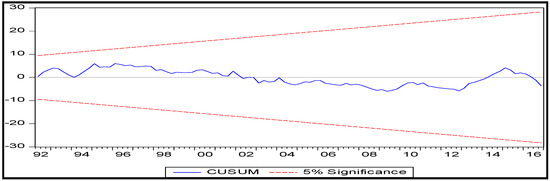
Figure 1.
CUSUM Test. Source: researcher’s computation based on Eviews 9.
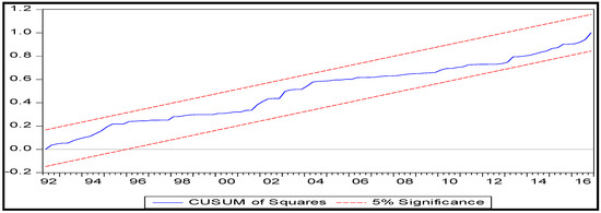
Figure 2.
CUSUM of Squares Test. Source: researcher’s computation based on Eviews 9.
5. Conclusions and Recommendations
The focus of the study was on analysing the impact of fiscal policy variables on economic growth in South Africa. Economic growth (GDP_RATE) was used as a dependent variable, and fiscal policy instruments were used as an independent variable. Empirical results revealed that public sector investment, tax revenue, terms of trade index, domestic private investment, real exchange rate, foreign direct investment, and portfolio investment have a positive influence on the GDP growth rate in South Africa, while high inflation and government consumption expenditure have a negative impact. The implication of these findings is that government expenditure does have a positive impact on growth, if it is of a capital nature rather than recurrent expenditure. This, therefore, suggests that an investment into infrastructure and any other related capital expenditure contributes to the growth of the South African economy. The government should therefore continue with more investment into infrastructure.
Author Contributions
Conceptualization, S.T. and A.T.; methodology, S.T.; software, S.T.; validation, S.T., F.M.K. and A.T.; formal analysis, S.T.; investigation, S.T.; resources, S.T.; data curation, S.T.; writing—original draft preparation, S.T.; writing—review and editing, S.T. and F.M.K.; visualization, S.T.; supervision, A.T. and S.T.; project administration, S.T.; funding acquisition, A.T. All authors have read and agreed to the published version of the manuscript.
Funding
This research received no external funding.
Institutional Review Board Statement
Not applicable.
Informed Consent Statement
Not applicable.
Data Availability Statement
Data available in a publicly accessible repository that does not issue DOIs Publicly available datasets were analyzed in this study. This data can be found on the South African reserve Bank data portal.
Conflicts of Interest
The authors declare no conflict of interest.
References
- Adegbite, Okebukola Hassan, and Tunde Owulabi. 2015. 1st National Finance and Banking Conference on Economic Reform and the Nigerian Financial System. A Communiqué read at National Conference organized by the Department of Finance. Lagos: University of Lagos. [Google Scholar]
- Ahmad, Manzoor, Shoukat Iqbal Khattak, Shehzad Khan, and Zia Ur Rahman. 2020. Do aggregate domestic consumption spending & technological innovation affect industrialization in South Africa? An application of linear & non-linear ARDL models. Journal of Applied Economics 23: 44–65. [Google Scholar]
- Akanbi, Olusegun Ayodele. 2013. Macroeconomic Effects of Fiscal Policy Changes: A Case of South Africa University of South Africa Pretoria, South Africa. Economic Modelling 35: 771–85. [Google Scholar] [CrossRef] [Green Version]
- Auerbach, Alan, and Laurence L. Kotlikoff. 1987. Dynamic Fiscal Policy. Cambridge: Cambridge University Press. [Google Scholar]
- Barro, Robert J. 1999. Economic Growth in a Cross Section of Countries. Quarterly Journal of Economics 106: 407–44. [Google Scholar] [CrossRef] [Green Version]
- Bhorat, Haroon, and Morné Oosthuizen. 2004. The Post-Apartheid South African Labour Market. Cape Town: University of Cape Town, Development Policy Research Unit. [Google Scholar]
- Brooks, Chris. 2008. Introductory Econometrics for Finance. Cambridge: Cambridge University Press. [Google Scholar]
- Cao, Quinton. 2006. Revision of the Tax Multiplier and Transfer Payment Multiplier in the Multiplier Theory. Ph.D. thesis, Southeast University, Nanjin, China. [Google Scholar]
- Christiano, Lawrence J., Martin Eichenbaum, and Robert Vigfusson. 2005. Assessing Structural VARs. NBER Macroeconomics Annual 21: 1–106. [Google Scholar] [CrossRef] [Green Version]
- Corden, Max. W. 1991. Does the Current Account Matter? The Old View and the New. Economic Papers 10: 119. [Google Scholar] [CrossRef]
- Dalyop, Gadong Toma. 2019. Political instability and economic growth in Africa. International Journal of Economic Policy Studies 13: 217–57. [Google Scholar] [CrossRef]
- DeLong, Bradford, and Lawrence Summers. 1991. Equipment investment and economic growth. Quarterly Journal of Economics 106: 445–502. [Google Scholar]
- Diamond, Peter A. 1965. National Debt in a Neoclassical Growth Model. The American Economic Review 55: 1126–50. [Google Scholar]
- Djelloul, Benanaya, Rachid Toumache, Abdallah Drif Rouaski, and Blessed Talbi. 2014. The impact of fiscal policy on economic growth: Empirical evidence from panel estimation. Paper presented at The 2014 WEI International Academic Conference Proceedings, New Orleans, LA, USA, October 19–22; Cambridge: Cambridge University Press. [Google Scholar]
- Duncan, Timothy, and Silvester Peter. 2008. Tariffs and non-traded goods. Journal of International Economics 4: 177–85. [Google Scholar]
- Fisher, Irving. 1993. The Role Macroeconomic Factors in Growth. Journal of Monetary Economics 32: 485–511. [Google Scholar] [CrossRef] [Green Version]
- Gaber, Stevan. 2009. Fiscal Stimulations for Improving the Business Environment in Republic of Macedonia. Perspectives of Innovations, Economics, and Business 3: 48–49. [Google Scholar] [CrossRef] [Green Version]
- Hauptmeier, Sebastian, Martin Heipertz, and Ludger Schuknecht. 2018. Expenditure Reform in Industrialized Countries: A Case Study Approach. Journal of Economic Studies 18: 3–30. [Google Scholar]
- Heitger, Blessing. 2018. The Scope of Government and Its Impact on Economic Growth in OECD Countries. Journal of Economic Literature 22: 38–39. [Google Scholar]
- Hlongwane, Themba, Itumeleng Pleasure Mongale, and Luzuko Tala. 2018. Analysis of the Impact of Fiscal Policy on Economic Growth in South Africa: VECM Approach. Journal of Economics and Behavioral Studies 10: 231–38. [Google Scholar] [CrossRef]
- International Monetary Fund. 2011. New Growth Drivers for Low-Income Countries: The Role of BRICs. Available online: http://www.imf.org/external/np/pp/eng/2011/011211.pdf (accessed on 10 May 2022).
- Karagianni, Stella, and Maria Pempetzogloub. 2012. Tax burden distribution and GDP growth: Non-linear causality considerations in the USA. International Review of Economics & Finance 12: 186–94. [Google Scholar]
- Kim, Adam, Robert King, and Simon Rodd. 2021. Will the New Keynesian Macroeconomics Resurrect the IS-LM Model? Journal of Economic Perspectives 7: 67–82. [Google Scholar]
- Liew, Venus Khim-Sen. 2004. What lag selection criteria should we employ? Journal of Academic Research in Economics 33: 1–9. [Google Scholar]
- López, Ralph, Thelma Vinod, and Young Wang. 2010. The Effect of Fiscal Policies on the Quality of Growth. Ph.D. thesis, Hubei Normal University, Shijiazhuang, China. [Google Scholar]
- M’Amanja, Daniel, and Oliver Morrissey. 2015. Fiscal Aggregates, Aid and Growth in Kenya. Nottingham: University of Nottingham. [Google Scholar]
- Mo, Pak Hung. 2007. Government Expenditures and Economic Growth: The Supply and Demand Sides. Fiscal Studies 28: 497–522. Available online: http://www.jstor.org/stable/24440029 (accessed on 10 May 2022). [CrossRef]
- Musgrave, Richard. 1959. Theory of Fiscal Policy. New York: McGraw Hill. [Google Scholar]
- Nie, Yemen, and Felix Ren. 2009. Mathematical Interpretation of the Different Tax Multiplier Results. Ph.D. thesis, Hubei Normal University, Shijiazhuang, China. [Google Scholar]
- Nourzad, Farrokh, and Martin Vrieze. 2017. Public Capital Formation and Productivity Growth: Some International Evidence. Journal of Productivity Analysis 6: 283–95. [Google Scholar] [CrossRef]
- Nuru, Naser Yenus, and Hayelom Yrgaw Gereziher. 2021. The effect of fiscal policy on economic growth in South Africa: A nonlinear ARDL model analysis. Journal of Economic and Administrative Sciences 38: 229–45. [Google Scholar] [CrossRef]
- Ocran, Matthew Kofi. 2011. Fiscal Policy and Economic Growth in South Africa. Paper presented at the Centre for the Study of African Economies “Conference on Economic Development in Africa”, Oxford, UK, March 22–24. [Google Scholar]
- Odhiambo, Nicholas M. 2009. Savings and economic growth in South Africa: A multivariate causality test. Journal of Policy Modeling 31: 708–18. [Google Scholar] [CrossRef]
- Pamba, Dumisani. 2021. The Effectiveness of Fiscal Policy on Economic Growth in South Africa: An Empirical Analysis. Ph.D. thesis, University of KwaZulu-Natal, Beria, South Africa. [Google Scholar]
- Parkin, Micheal, Steven Antrobus, Neethling Peter Baur, Jeffrey Bruce-Brand, Kirsten Thompson, and Dirk Scholtz. 2012. Global and Southern African Perspectives. Economics: Pearson Education South Africa (Pty) Ltd. [Google Scholar]
- Perman, Roger. 1991. Cointegration: An Introduction to the Literature. Journal of Economic Studies 18: 3–30. [Google Scholar] [CrossRef]
- Perotti, Roberto. 2007. In Search of the Transmission Mechanism of Fiscal policy. NBER Macroeconomics Annual 22: 169–226. [Google Scholar] [CrossRef]
- Pesaran, Mohammad Hashem, and Bigan Pesara. 1997. Working with Microfit 4.0: Interactive Econometric Analysis (User’s Manual). Oxford: Oxford University Press. [Google Scholar]
- Ramey, Valerie A. 2011. Can Government Purchases Stimulate the Economy? Journal of Economic Literature 49: 673–85. [Google Scholar] [CrossRef] [Green Version]
- Rodrik, Dani. 2007. Introductiion to One Economics, Many Recipes: Globalization, Institutions, and Economic Growth. In One Economics, Many Recipes: Globalization, Institutions, and Economic Growth. Princeton: University Press. [Google Scholar]
- Romer, Paul. M. 1986. Increasing Returns and Long-run Growth. Journal of Political Economy 94: 1002–37. [Google Scholar] [CrossRef] [Green Version]
- Shahbaz, Modric, Adam Jalil, and Felix Islam. 2010. Real Exchange Rate Changes and Trade Balance in Pakistan: A Revisit. Munich: University of Munich. [Google Scholar]
- South African Reserve Bank. 2016. Excellence in Price and Financial Stability. Annual Report 2015/16. Available online: https://resbank.onlinereport.co.za/2016-annual-reports (accessed on 10 June 2020).
- Taylor, John B. 2009. The Lack of an Empirical Rationale for a Revival of Discretionary Fiscal Policy. American Economic Review: Papers and Proceedings 99: 550–55. [Google Scholar] [CrossRef] [Green Version]
- Treasury. 2017. The South African Tax Reform Experience since 1994. Address by the Honourable Trevor A Manuel, MP. Minister of Finance. Annual Conference of the International Bar Association. Available online: http://www.treasury.gov.za/comm_media/speeches/2002/2002102501.pdf (accessed on 10 February 2021).
- Uremadu, Sebastian Ofumbia. 2012. The Impact of Real Interest Rate on Savings Mobilization in Nigeria. Unpublished. Ph.D. thesis, University of Nigeria, Nsukka, Nigeria. [Google Scholar]
- Van der Berg, Servaas. 2010. Current Poverty and Income Distribution in the Context of South African History: Stellenbosch Economic. Working Papers. Stellenbosch: Stellenbosch University, Department of Economics, vol. 22, pp. 38–39. [Google Scholar]
Publisher’s Note: MDPI stays neutral with regard to jurisdictional claims in published maps and institutional affiliations. |
© 2022 by the authors. Licensee MDPI, Basel, Switzerland. This article is an open access article distributed under the terms and conditions of the Creative Commons Attribution (CC BY) license (https://creativecommons.org/licenses/by/4.0/).