The Effect of Interest Rate Changes on Consumption: An Age-Structured Approach

Abstract

Interest rates have generally trended downward over the past several decades. It has made borrowing cheaper, which has encouraged people to spend more. It has also made saving less attractive, contributing to increased consumption. At the same time, the role of household credit increased significantly. The paper suggests a model for the effect of an interest rate change on household consumption, which relies on income and loans. The model is based on methods of the optimal control theory. The approach is age-structured: households reconsider their consumption patterns at the moment of the interest rate change and the changes in consumption patterns are age dependent. The consumption changes for different age groups contribute to the modification of aggregate consumption. Numerical simulation shows that a decrease in the interest rate leads to a consumption boost (a substantial increase in consumption in the short run), which diminishes as time passes and consumption becomes fully adjusted to the new interest rate value. The consumption boost is achieved by an increase in the debt load.

1. Introduction

Consumption theories attempt to explain and predict patterns of consumer spending. These theories are critical because consumer spending plays a central role in the economy, as it drives demand for goods and services and can significantly impact economic growth.

There are different consumption theories, including:

• The Keynesian Consumption Function Keynes (1936): This theory, developed by economist John Maynard Keynes, suggests that consumer spending is driven by disposable income.
• The Permanent Income Hypothesis Friedman (1957): This theory, developed by economist Milton Friedman, suggests that consumer spending is not solely driven by current disposable income, but also by the individual’s expected lifetime income. According to this theory, consumers will adjust their spending to match their expected lifetime income, rather than just their current income.
• The Life Cycle Hypothesis Ando and Modigliani (1963); Modigliani and Brumberg (1954): This theory, developed by economist Franco Modigliani, suggests that consumer spending is influenced by an individual’s life stage and expected future income. According to this theory, younger individuals are more likely to have higher levels of debt and lower levels of savings, while older individuals are more likely to have higher levels of savings and lower levels of debt.

These theories are not mutually exclusive. Consumer behavior can be influenced by a wide range of factors, including inflation rates, taxes, wage levels, government policies, macroeconomic shocks, and expectations about the future. Recent development covers the role of labor income uncertainty Carroll (1994); Gourinchas and Parker (2002), the influence of wealth Alp and Seven (2019), sustainability issues Hertwich (2005), the effects of stimulus payments Kaplan and Violante (2014), the specifics of developing countries Van Tran (2022), etc. The focus of the present paper is the effect of the interest rate changes Cloyne et al. (2020); Navarro and de Frutos (2015) and household debt growth Coskun et al. (2022); Kapeller and Schutz (2014).

Households’ spending is often financed by borrowing. It is particularly relevant for housing and durables. Consumption of services and nondurables can also rely on credit, especially in developed countries. During past decades, there were generally decreasing interest rates and easy access to credit. These two factors have a substantial effect on household consumption. In general, higher interest rates discourage consumption and encourage saving. Lower interest rates encourage consumption and discourage saving because there is less point in saving money. When interest rates decrease, it becomes cheaper for individuals to borrow money, which can encourage them to consume more. In this case, when borrowing money is cheaper, individuals may be more willing to take on debt to finance their consumption. In the past, credit was mainly used for large purchases such as homes or cars. The widespread availability of credit in many countries has also made it easier for people to borrow money for various purposes, such as paying for education, medical expenses, and vacation financing. Overall, credit has become an integral part of modern economies, and it is likely that its role will continue to grow in the future.

To illustrate the growth of credit, we use data for the USA: Figure 1 shows the increasing role of consumer credit. The rise of household debt and its relevance to consumption growth were analyzed in Barba and Pivetti (2009); Christen and Morgan (2005); Wolff (2011). It should be noted that the growth of household debt is common in many countries Johnston at al. (2021); Mian et al. (2017). At the same time, a significant fraction of households save little or no liquid wealth (see Leung (2000) and references therein). The growth of credit is tightly linked to interest rates. The level of interest rates is often seen as a critical driver of credit growth. In the case of the USA, it can be easily seen in the interest rates data in Figure 2 and in the USA government bonds data in Figure 3. Figure 2 shows several steep drops and gradual increases in interest rates. The general trend for the interest rates during past decades, let us say that from the 1980s, was the decline from high (double-digit) values to values close to zero. Substantial decreases in interest rates are usually implemented to stimulate consumption and business activities in times of economic difficulties. For example, the last substantial decrease took place because of the financial crisis of 2007–2009. The last but one was related to the dot-com bubble of 2000. Inevitably, such changes affected the consumption pattern.

The intertemporal relationship between the interest rates and consumption (saving) attracted many economists Carlino (1982); Fortune and Ortmeyer (1985); Gylfason (1981); Taylor (1999). A particular topic is the effect of interest rate shocks on consumption Cloyne et al. (2020); Coskun et al. (2022). The impact of interest rate changes on consumption needs to be understood, in particular, for efficient implementation of monetary policy. There were comparatively few empirical attempts to study the effect of the interest rate changes on consumption, moreover, incredibly few attempts to approach this topic at a disaggregated level. Most of the authors argue in favor of the inverse relation between changes in consumption and interest rates. They also argue that it is appropriate to consider the real (not nominal) interest rate. In Carlino (1982); Gylfason (1981), it was discussed that some results of the empirical studies are inconsistent. It should be noted that most of the known results were established before low interest rates became the new reality during the past two decades.

Falling mortgage rates can be used for refinancing that frees up disposable income for additional consumption Tauheed and Wray (2006). In Di Maggio et al. (2017), the authors considered the effects of lower mortgage rates on consumption and mortgage downpayments. Car purchases were used as the primary measure of consumption. It was found that a substantial decline in mortgage payments (up to 50%) led to a noticeable increase in car purchases (up to 35%).

In this paper, we suggest a model for the effect of an interest rate change on total consumption (both durable and nondurable goods). We consider households that rely on income and loans (student loans, mortgage loans, car loans, credit cards, etc.), assuming that a household behaves as a unit. Households can borrow against future earnings to optimize consumption over their life cycles. There are no restrictions on saving and borrowing. The borrowing strategies depend on the interest rates. For this reason, the interest rate decrease can be an efficient tool for consumption stimulation.

Of course, the analysis of the impact of the interest rate changes needs to be based on comprehensive economic development models, which include all relevant factors such as firms, government spending, taxation, public debt, economic growth, technological development, etc. All these factors make the analysis very complicated, mainly because it is difficult to make future predictions for some of these factors. We substitute this complicated problem with a more straightforward problem: Which effect can an interest rate change have on consumption provided that the other conditions (employment, labor income, the value of assets, etc.) remain the same? The only other parameter which can be changed is the subjective discount rate, which is induced by the interest rate value. The analysis does not take into account the reasons for the interest rate change.

For further simplification, we consider only households in the labor force because, for them, the consumption changes are expected to be the most significant (both consumption and the flexibility to change consumption patterns drop at retirement). These households are divided into age groups. The effect of interest rates on consumption can depend on a variety of factors, including the individual’s age, income, and wealth. It is reasonable to assume that younger people can have more possibilities to benefit from lower interest rates than older people, as they have more time to take advantage of the lower borrowing costs. Thus, the age-structured approach is a natural choice for modeling the effect of interest rates on consumption. Age-structured models are popular in a variety of fields, including macroeconomics. These models are based on the idea that a population can be divided into different age groups, each with specific characteristics and behaviors. The households are divided into age groups. At the moment of the interest rate change, households from different age groups change their consumption patterns. These consumption changes contribute to the modification of aggregate consumption.

Modeling a representative household from a particular age group is based on methods of optimal control theory. Optimal control theory is a mathematical tool used to analyze the behavior of systems that change over time. It is instrumental in macroeconomics, where it can be used to study the behavior of aggregate economic variables Caputo (2005); Kamien and Schwartz (2012); Sierstad and Sydsaeter (1987); Weber (2011). Control theory can also be used to design and implement policy interventions to stabilize the economy or achieve specific economic goals. For example, control theory can be used to design feedback mechanisms that can automatically adjust policy in response to changes in economic conditions, such as changes in inflation or unemployment. To our knowledge, there have been no attempts to combine the age-structured approach and optimal control theory to analyze the effect of interest rate changes on household consumption. The standard approach uses methods of control theory for infinitely living households.

Several simplifying assumptions help to isolate the interest rate effect and to provide a high degree of analytical tractability. We assume that the interest rate was constant for a long time. Then, it is changed to another value, which will be held for a long time. This change is unexpected for households and makes them reconsider their consumption patterns. Of course, this scenario is a substantial simplification of reality. In real life, interest rate changes happen relatively often, and the interest rate cannot be assumed to be constant for a long time. People also have expectations for interest rate dynamics, at least for the nearest future. However, the considered approach can reveal some essential features of the interest rate effect on consumption.

All representative households for particular age groups stay the same number of years in the labor force. They start with some initial debt and finish working life with some savings. To simplify further, we assume no demographic changes—the same number of households join and quit the labor force every year.

The focus of the paper is devoted to the effect of interest rate changes on consumption. There are several practical reasons for such an analysis. Probably, the most important is understanding the stimulating effect of an interest rate decrease on consumption. On the other hand, there are concerns related to the reverse changes, namely possible increases in low interest rates. High levels of household debt can pose risks, as they can lead to financial instability and make it more difficult to manage financial challenges in the future. Household debt increased during the last decades relative to disposable income and bank deposits Gerdrup and Torstensen (2018). An increase in the interest rate will reduce disposable income more than previously. It will lead to a follow-up decrease in consumption.

The paper is organized as follows. In Section 2, we describe a basic model for a constant value of the interest rate. This model reflects how the consumption rate and the debt load depend on the interest rate and the subjective discounting rate. Section 3 introduces an interest rate change as a parameter change for the basic model. Numerical simulations for the effect of the interest rate decrease (and increase) on consumption and debt are provided in Section 4. Section 5 provides a discussion of the computational results. Finally, Section 6 presents concluding remarks concerning future research directions. Some technical results are separated into Appendix A and Appendix B.

2. The Basic Model

This section presents a basic model for a constant interest rate. The model describes a representative household for a particular age group. This representative household can be considered an average household for the age group. Changes in the interest rate will be introduced in the forthcoming section.

2.1. Model Formulation

All households are assumed to stay in the labor force for T years (time will be measured in years). The starting year for a particular age group is denoted as $t_0$. Such households will be in the labor force during the time interval $[t_0,t_0+T]$. The representative household chooses a consumption plan $C\left(t\right)>0$ to maximize the total utility value, which is given by the integral of the discounted utility rate over the the time interval $[t_0,t_0+T]$

$$\underset{C\left(t\right)>0}{\max }{\int }_{t_0}^{t_0+T}\alpha \left(t\right)U\left(C\left(t\right)\right)dt.$$

(1)

Here, $\alpha \left(t\right)$ is a discount function and $U\left(C\right)$ is a utility function.

The standard choice is the exponential discount function

$$\alpha \left(t\right)=e^{-\delta t},$$

(2)

where $\delta >0$ is the subjective rate of discount. It should be noted that for the borrowing scenario, we expect $\delta >r$, where r is the constant interest rate.

The utility function is taken in the exponential form

$$U\left(C\right)=U_1\left(C\right)=1-e^{-C}.$$

(3)

Two other popular choices are the logarithmic

$$U_2\left(C\right)=lnC$$

(4)

and power

$$U_3\left(C\right)=\frac{1}{1-\gamma }{C}^{1-\gamma },0<\gamma <1$$

(5)

utility functions. All three utility functions are compared in Appendix A. The utility function (3) gives linear $C\left(t\right)$ for the considered optimal control problem that simplifies the analysis as well as the visualization of the results.

Remark 1.

Instead of utility function (3) it is more appropriate to consider the utility function

$$U_1\left(C\right)=1-e^{-C/w_0},$$

where $w_0$ is a parameter. The value $w_0=1$ suits the other parameters well, and will be used for numerical simulation. That is why we omit $w_0$ and continue with (3).

The consumption rate, the loan value, and the income rate are related by the ordinary differential equation,

$$K^{\prime }\left(t\right)=rK\left(t\right)+C\left(t\right)-w.$$

(6)

This equation states that the consumption is provided by earned income, given by the constant income rate w, and borrowing against future earnings. We denote the loan value as $K\left(t\right)$ assuming that it describes borrowing if $K\left(t\right)>0$ and saving if $K\left(t\right)<0$. For households starting in the labor force at year $t_0$ there are boundary conditions,

$$K\left(t_0\right)=K^0,K(t_0+T)=K^T.$$

(7)

Here, $K^0$ and $K^T$ are constant. They denote the loan values at the initial time $t_0$ and at the final time $t_0+T$. As mentioned before, negative values can also be considered; they are interpreted as savings. For example, a positive value $K^0$ can stand for a student loan and a negative value $K^T$ can be saving for retirement.

Remark 2.

For simplicity, the suggested framework assumes that the income rate, initial, and final loan are constant. In a more general case, they can be time-dependent functions,

$$w(t,t_0),K^0\left(t_0\right)and{K}^T\left(t_0\right).$$

We summarize the basic model as the following consumption–borrowing/saving problem: The households optimize borrowing/saving during T years expressed by the maximization of the functional (1) subject to the dynamic relation (6) and the boundary conditions (7).

2.2. Solution of the Control Problem

There are many textbooks on control problems and their applications Caputo (2005); Kamien and Schwartz (2012); Pontryagin et al. (1962); Sierstad and Sydsaeter (1987); Weber (2011). The equations for the optimal control problem (1), (6) are provided by the Hamiltonian function,

$$H=e^{-\delta t}U\left(C\left(t\right)\right)+\lambda \left(t\right)(rK\left(t\right)+C\left(t\right)-w).$$

(8)

Here, we assume that there is no need to care about the constraint $C\left(t\right)>0$. Otherwise, this constraint should be added to the Hamiltonian function (and the system would have more equations).

The Hamiltonian leads to the system of equations,

$$\begin{array}{c}{K}^{\prime }\left(t\right)=H_{\lambda },\end{array}$$

(9a)

$$\begin{array}{c}{\lambda }^{\prime }\left(t\right)=-H_K,\end{array}$$

(9b)

$$\begin{array}{c}{H}_C=0,\end{array}$$

(9c)

which takes the form

$$\begin{array}{c}{K}^{\prime }\left(t\right)=rK\left(t\right)+C\left(t\right)-w,\end{array}$$

(10a)

$$\begin{array}{c}{\lambda }^{\prime }\left(t\right)=-r\lambda \left(t\right),\end{array}$$

(10b)

$$\begin{array}{c}{e}^{-\delta t}{U}^{\prime }\left(C\left(t\right)\right)+\lambda \left(t\right)=0.\end{array}$$

(10c)

We denote the consumption rate and the loan value for the system of Equations (10a)–(10c) with the boundary conditions (7) as

$$C(t,t_0)\mathrm{and}K(t,t_0).$$

(11)

Here, time t is the independent variable and $t_0$ stands as a parameter. For the utility function $U_1$, given in (3), the consumption rate and the loan value for the starting year $t_0$ are

$$C(t,t_0)=w+(r-\delta )T\left(\frac{t-t_0}{T}+\frac{1}{e^{rT}-1}-\frac{1}{rT}\right)+r\frac{K^T-e^{rT}{K}^0}{e^{rT}-1}$$

(12)

and

$$\begin{array}{c}\hfill K(t,t_0)=\frac{\delta -r}{r}T\left(\frac{t-t_0}{T}-\frac{e^{r(t-t_0)}-1}{e^{rT}-1}\right)+K^0\frac{e^{rT}-e^{r(t-t_0)}}{e^{rT}-1}+K^T\frac{e^{r(t-t_0)}-1}{e^{rT}-1}.\end{array}$$

(13)

Note that the convenient choice of the utility function makes $C(t,t_0)$ linear in time t.

2.3. Aggregation for Age Groups

The solution of the control problem leads to several important averaged quantities for the whole time in the labor force, i.e., over the interval $[t_0,t_0+T]$:

• The average consumption rate

  $$\overline{C}\left([t_0,t_0+T]\right)=\frac{1}{T}{\int }_{t_0}^{t_0+T}C(t,t_0)dt;$$

  (14)
• The average loan value

  $$\overline{K}\left([t_0,t_0+T]\right)=\frac{1}{T}{\int }_{t_0}^{t_0+T}K(t,t_0)dt;$$

  (15)
• The payment for the loan (this short name, which is relevant only for the case $K^T=K^0$, is used for convenience)

  $$P\left([t_0,t_0+T]\right)={\int }_{t_0}^{t_0+T}wdt-{\int }_{t_0}^{t_0+T}C(t,t_0)dt=T(w-\overline{C}\left([t_0,t_0+T]\right)).$$

  (16)

For the solution (12), (13) these average values are

$$\overline{C}\left([t_0,t_0+T]\right)=w+(r-\delta )T\left(\frac{1}{2}+\frac{1}{e^{rT}-1}-\frac{1}{rT}\right)+r\frac{K^T-e^{rT}{K}^0}{e^{rT}-1},$$

(17)

$$\overline{K}\left([t_0,t_0+T]\right)=\frac{\delta -r}{r}T\left(\frac{1}{2}+\frac{1}{e^{rT}-1}-\frac{1}{rT}\right)+\frac{e^{rT}{K}^0-K^T}{e^{rT}-1}+\frac{K^T-K^0}{rT},$$

(18)

$$P\left([t_0,t_0+T]\right)=(\delta -r)T^2\left(\frac{1}{2}+\frac{1}{e^{rT}-1}-\frac{1}{rT}\right)+rT\frac{e^{rT}{K}^0-K^T}{e^{rT}-1},$$

(19)

respectively. Note that for $K^0=K^T=0$ we have

$$P\left([t_0,t_0+T]\right)=rT\overline{K}\left([t_0,t_0+T]\right).$$

Another set of average values corresponds to a particular time t for which we make averaging over all age groups. We recall that there are no demographic changes. At some particular time t, the average consumption rate and the average loan value are contributed by the age group with starting time $t_0$ satisfying $t-T<t_0<t$:

$$\overline{C}\left(t\right)=\frac{1}{T}{\int }_{t-T}^{t}C(t,t_0)d{t}_0,$$

(20)

$$\overline{K}\left(t\right)=\frac{1}{T}{\int }_{t-T}^{t}K(t,t_0)d{t}_0.$$

(21)

It is also possible to consider the aggregate consumption rate, which is proportional to the average consumption rate in the considered framework.

We obtain

$$\overline{C}\left(t\right)=w+(r-\delta )T\left(\frac{1}{2}+\frac{1}{e^{rT}-1}-\frac{1}{rT}\right)+r\frac{K^T-e^{rT}{K}^0}{e^{rT}-1},$$

(22)

$$\overline{K}\left(t\right)=\frac{\delta -r}{r}T\left(\frac{1}{2}+\frac{1}{e^{rT}-1}-\frac{1}{rT}\right)+\frac{e^{rT}{K}^0-K^T}{e^{rT}-1}+\frac{K^T-K^0}{rT}.$$

(23)

For the assumptions made, we get

$$\overline{C}\left(t\right)=\overline{C}\left([t_0,t_0+T]\right),$$

(24)

$$\overline{K}\left(t\right)=\overline{K}\left([t_0,t_0+T]\right).$$

(25)

However, equality relations (24) and (25) can fail to hold for more general models.

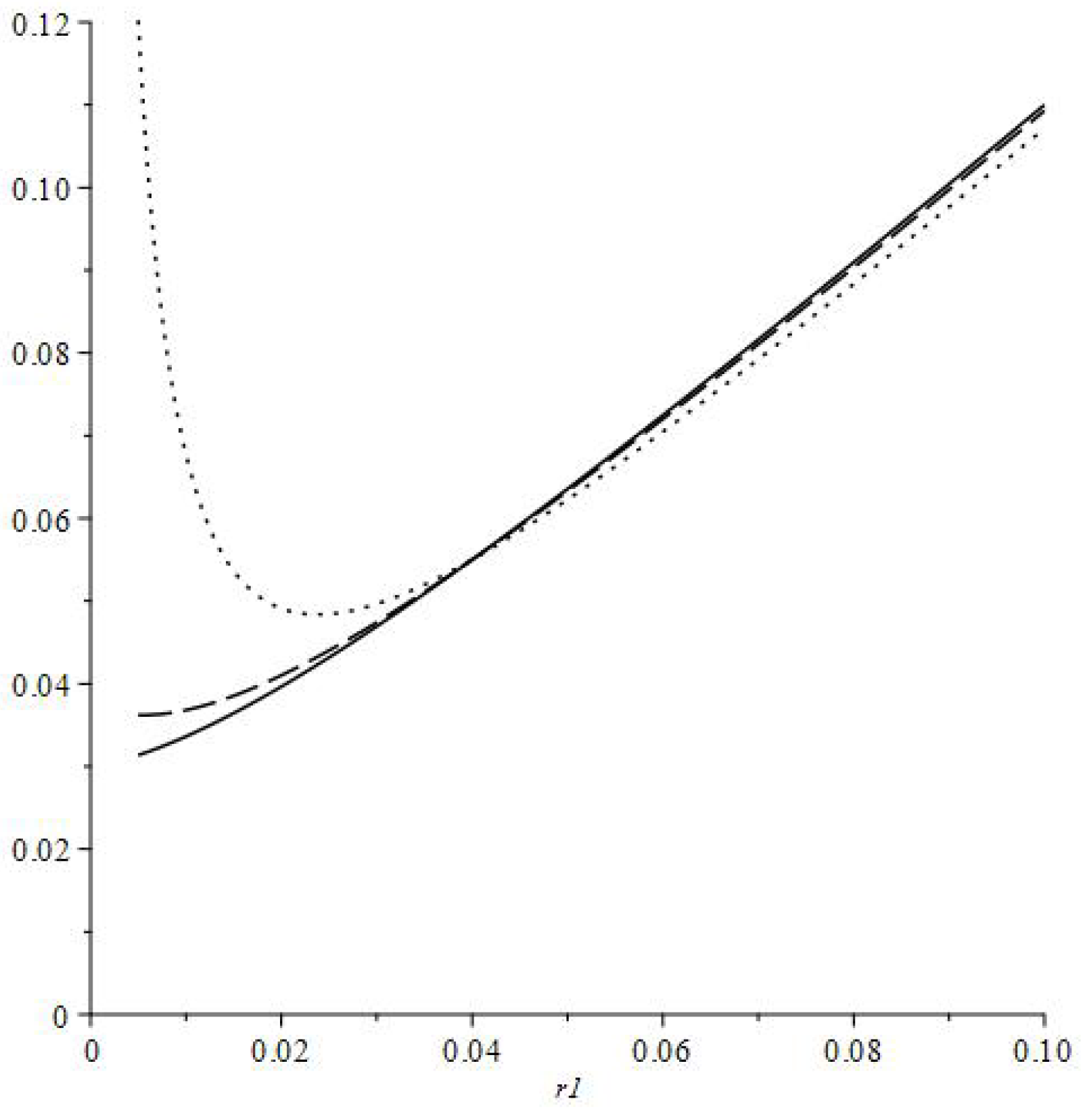
2.4. Calibration of the Discount Rate $\delta$

For modeling, it is necessary to choose the subjective rate of discount $\delta$ for the discount function (2). Here one can make use of the maximal loan value and the average quantities of the model, such as the average loan value (15) and the loan payment (16). We suggest specifying a convex combination of these quantities as a multiplum of the annual income:

$${\alpha }_1\underset{t\in [t_0,t_0+T]}{\max }K(t,t_0)+{\alpha }_2\overline{K}\left([t_0,t_0+T]\right)+{\alpha }_{3}P\left([t_0,t_0+T]\right)=\beta w,$$

$${\alpha }_1,{\alpha }_2,{\alpha }_3\ge 0,{\alpha }_1+{\alpha }_2+{\alpha }_3=1,\beta >0.$$

Here, all ${\alpha }_i$ and $\beta$ are constants.

Several possibilities can be easily selected:

• ${\alpha }_1=1$, ${\alpha }_2={\alpha }_3=0$: the maximal loan value

  $$\underset{t\in [t_0,t_0+T]}{\max }K(t,t_0)=\beta w;$$

  (26)
• ${\alpha }_1={\alpha }_3=0.5$, ${\alpha }_2=0$: the sum of the maximal loan value and the loan payment

  $$\underset{t\in [t_0,t_0+T]}{\max }K(t,t_0)+P\left([t_0,t_0+T]\right)=2\beta w;$$

  (27)
• ${\alpha }_2={\alpha }_3=0.5$, ${\alpha }_2=0$: the sum of the average loan value and the loan payment

  $$\overline{K}\left([t_0,t_0+T]\right)+P\left([t_0,t_0+T]\right)=2\beta w.$$

  (28)

The analytical expression for the maximal value of $K(t,t_0)$ for $t\in [t_0,t_0+T]$ is provided in Appendix B.

This section provided the solution to the control problem and the associated average quantities for the utility function (3). One can employ the other utility functions (4) and (5) in a similar manner.

3. Interest Rate Changes

Now we incorporate interest rate changes into the basic model, presented in the previous section. The general description of the approach is supplemented by particular results for the exponential utility function (3).

First we consider the change of a pair $(r,\delta )$, which consists of the interest rate and the discount rate, from the original values $(r_0,{\delta }_0)$ to new values $(r_1,{\delta }_1)$. Determination of ${\delta }_1\left(r_1\right)$ is considered separately.

3.1. Particular Age Groups

We assume that the interest rate had a long-time value $r_0$. Then at some time, which we denote by $t=0$ for convenience, the interest rate is changed from $r_0$ to a new value $r_1$, which will be held for a long time. There are three types of behavior for the consumption rate $C(t,t_0)$ and the loan $K(t,t_0)$:

• Only with the interest rate $r_0$ if $t_0\le -T$;
• With both interest rates $r_0$ and $r_1$ if $-T<t_0<0$;
• Only with the interest rate $r_1$ if $t_0\ge 0$.

The solutions for these three cases are the following:

• Case $t_0\le -T$ (before the transition)
  The consumption rate $C_0(t,t_0)$ and the loan $K_0(t,t_0)$ are given by the basic model (12) and (13) with $r=r_0$ and $\delta ={\delta }_0$, namely

  $$C_0(t,t_0)={\left.C(t,t_0)\right|}_{r=r_0,\delta ={\delta }_0},K_0(t,t_0)={\left.K(t,t_0)\right|}_{r=r_0,\delta ={\delta }_0}.$$

  (29)
• The transition case $-T<t_0<0$.
  The interval $(t_0,t_0+T)$ includes the moment of the interest rate change $t=0$. The interval is split into two subintervals: $(t_0,0)$ with the interest rate $r_0$ and $(0,t_0+T)$ with the interest rate $r_1$.

  (a)

  $t\in (t_0,0)$.

  For the interval $(t_0,0)$, the results are the same as for the case $t_0\le -T$:

  $$C_1(t,t_0)=C_0(t,t_0),K_1(t,t_0)=K_0(t,t_0),t_0<t<0,$$

  see (29) for $C_0(t,t_0)$ and $K_0(t,t_0)$.

  At the end of this interval, i.e., at time $t=0$, the household has the loan

  $$\widehat{K}=K_1(0,t_0)=K_0(0,t_0).$$

  (30)

  (b)

  At the time $t=0$, there is a change of the interest rate r and an induced change of the rate of discount $\delta$. The new values are $r_1$ and ${\delta }_1$. We assume that parameter ${\delta }_0$ was fitted as described in Section 2.4. The determination of the parameter ${\delta }_1$ is a separate subproblem, which will be discussed in the next subsection.

  At $t=0$, there is a switch from the control problem Equations (10a)–(10c) with $r=r_0$, $\delta ={\delta }_0$ and boundary conditions (7) to the Equations (10a)–(10c) with $r=r_1$, $\delta ={\delta }_1$ and the modified boundary conditions (31).

  (c)

  $t\in (0,t_0+T)$

  For the rest, i.e., on the interval $(0,t_0+T)$, the dynamic is given by Equations (10a)–(10c) with $r_1$ and ${\delta }_1$. The boundary conditions are

  $$K_1(0,t_0)=\widehat{K},K_1(t_0+T,t_0)=K^T,$$

  (31)

  where

  $$\widehat{K}=\frac{{\delta }_0-r_0}{r_0}T\left(-\frac{t_0}{T}-\frac{e^{-r_0{t}_0}-1}{e^{r_{0}T}-1}\right)+K^0\frac{e^{r_{0}T}-e^{-r_0{t}_0}}{e^{r_{0}T}-1}+K^T\frac{e^{-r_0{t}_0}-1}{e^{r_{0}T}-1}.$$

  The solution is given by the consumption rate,

  $$C_1(t,t_0)=w+(r_1-{\delta }_1)\left(t+\frac{t_0+T}{e^{r_1(t_0+T)}-1}-\frac{1}{r_1}\right)+r_1\frac{K^T-e^{r_1(t_0+T)}\widehat{K}}{e^{r_1(t_0+T)}-1}$$

  and the loan value

  $$\begin{array}{c}{K}_1(t,t_0)=\frac{{\delta }_1-r_1}{r_1}\left(t-(t_0+T)\frac{e^{r_{1}t}-1}{e^{r_1(t_0+T)}-1}\right)\hfill \\ +\widehat{K}\frac{e^{r_1(t_0+T)}-e^{r_{1}t}}{e^{r_1(t_0+T)}-1}+K^T\frac{e^{r_{1}t}-1}{e^{r_1(t_0+T)}-1}.\hfill \end{array}$$

  Note that $\widehat{K}$ is a function of several parameters and $K^T$ is a constant.

• Case $t_0\ge 0$ (after the transition)
  Here, $C_2(t,t_0)$ and $K_2(t,t_0)$ are given by the basic model (12) and (13) with $r=r_1$ and $\delta ={\delta }_1$, i.e., they are

  $$C_2(t,t_0)={\left.C(t,t_0)\right|}_{r=r_1,\delta ={\delta }_1},K_2(t,t_0)={\left.K(t,t_0)\right|}_{r=r_1,\delta ={\delta }_1}.$$

  (32)

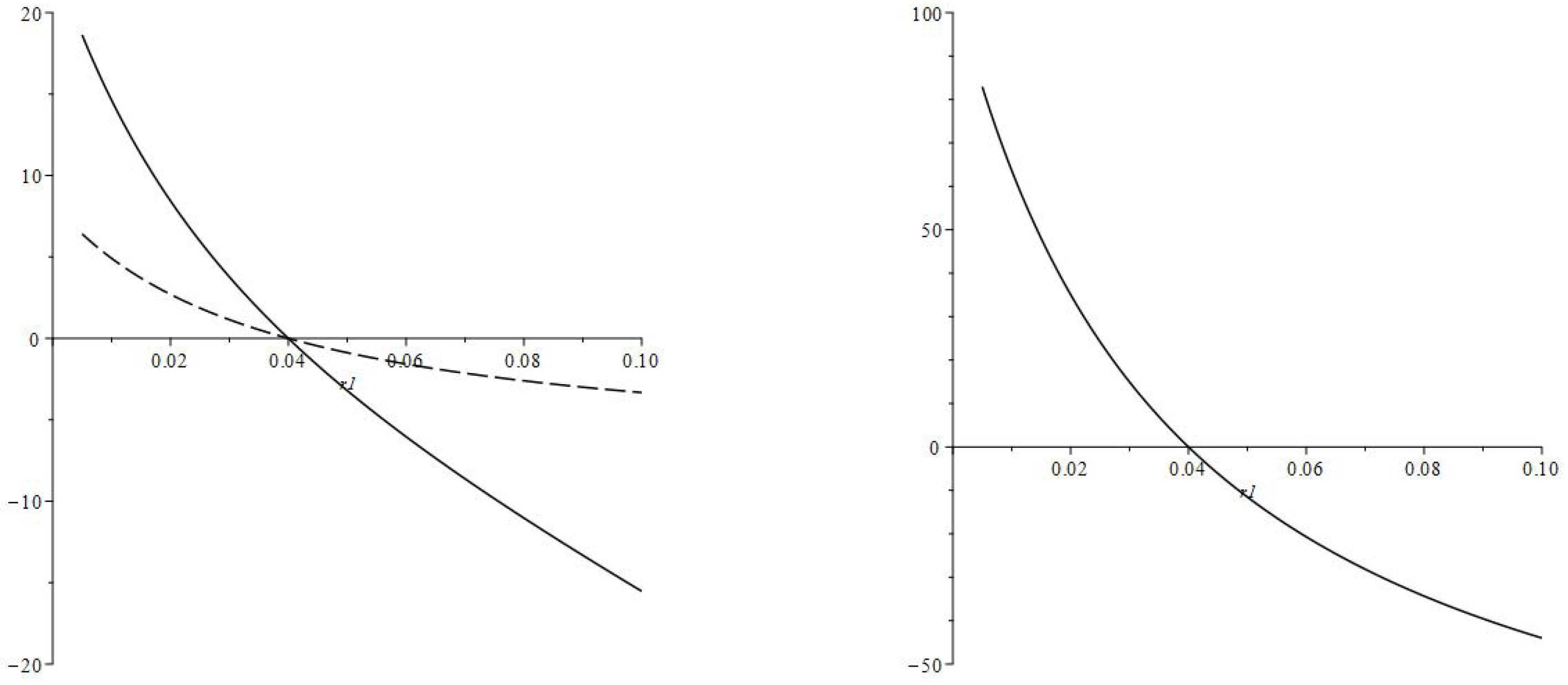
3.2. Determination of the New Discount Rate ${\delta }_1$

When the interest rate is changed from $r_0$ to $r_1$, it induces the change of the discount rate from ${\delta }_0$ to ${\delta }_1$. We suggest finding ${\delta }_1$ from the following relation for quantities characterizing the old and new cases.

$${\alpha }_1\max K_2+{\alpha }_2{\overline{K}}_2+{\alpha }_3{P}_2={\alpha }_1\max K_0+{\alpha }_2{\overline{K}}_0+{\alpha }_3{P}_0,$$

$${\alpha }_1,{\alpha }_2,{\alpha }_3\ge 0,{\alpha }_1+{\alpha }_2+{\alpha }_3=1.$$

Here, $\max K_i$ is the maximal loan value, ${\overline{K}}_i$ is the average loan value and $P_i$ is the payment for the loan. Index $i=2$ is used for the new values (upon completion of the transition).

$$\begin{array}{cc}\max K_2=\underset{t\in [t_0,t_0+T]}{\max }{K}_2(t,t_0),{\overline{K}}_2=\overline{K}\left([t_0,t_0+T]\right),\hfill & \\ & \hfill P_2=P_2\left([t_0,t_0+T]\right),t_0\ge 0.\end{array}$$

Index value $i=0$ is used for the original values.

$$\begin{array}{cc}\max K_0=\underset{t\in [t_0,t_0+T]}{\max }{K}_0(t,t_0),{\overline{K}}_0=\overline{K}\left([t_0,t_0+T]\right),\hfill & \\ & \hfill P_0=P_0\left([t_0,t_0+T]\right)t_0\le -T.\end{array}$$

The maximal values are discussed in Appendix B, the values ${\overline{K}}_i$ and $P_i$ are given in (15) and (16). Note that a particular choice of $t_0$ for $t_0\ge 0$ or $t_0\le -T$ does not matter for the considered model.

In the next section, the following methods will be tested to find ${\delta }_1\left(r_1\right)$:

• ${\alpha }_1={\alpha }_3=0.5$, ${\alpha }_2=0$.
  Here, the new and original values $(r,\delta )$ are related by assumption that the sum of the maximal loan value and the loan payment is the same for new values $r_1$ and ${\delta }_1$ as it was for the original values $r_0$ and ${\delta }_0$, i.e.,

  $$\max K_2+P_2=\max K_0+P_0;$$

  (33)
• ${\alpha }_2={\alpha }_3=0.5$, ${\alpha }_1=0$
  Similarly, we can use the sum of the average loan value and the payment:

  $${\overline{K}}_2+P_2={\overline{K}}_0+P_0;$$

  (34)
• ${\alpha }_3=1$, ${\alpha }_1={\alpha }_2=0.$
  For completeness, we can also consider

  $$P_2=P_0.$$

  (35)
  This approach does not suit small values $r_1$ because

  $$P_2\approx \frac{T^3}{12}({\delta }_1-r_1)r_1+K^0\left(1+\frac{r_{1}T}{2}\right)-K^T\left(1-\frac{r_{1}T}{2}\right)$$

  and

  $$P_2\to K^0-K^{T}as{r}_1\to 0.$$

Remark 3.

It might also be interesting to consider the unchanged discount rate:

$${\delta }_1={\delta }_0.$$

However, this makes sense only for minimal interest rate changes $r_1\approx r_0$.

3.3. Averaging for All Age Groups

The average consumption rate and the average loan value at some time t depend on contributions from households of the age groups with $t_0$ satisfying $t-T\le t_0\le t$. We recall that there are no demographic changes. There are three cases for such averaging depending on time t.

• Case $t\le 0$ (before the interest rate change)
  Only households with $t_0\le -T$ contribute. In this case

  $${\overline{C}}_0\left(t\right)={\overline{C}}_0=\frac{1}{T}{\int }_{t-T}^t{C}_0(t,t_0)d{t}_0,t_0\le -T$$

  (36)

  and

  $${\overline{K}}_0\left(t\right)={\overline{K}}_0=\frac{1}{T}{\int }_{t-T}^t{K}_0(t,t_0)d{t}_0,t_0\le -T$$

  (37)

  are actually constant. These quantities are given by (22) and (23) with $r=r_0$ and $\delta ={\delta }_0$.
• Case $0<t<T$ (the transition of the consumption patterns)
  The households are divided into two groups: households with $t-T<t_0<0$, changing their behavior at $t=0$, and households with $0\le t_0<t$, joining the labor force under the new conditions, i.e., with the interest rate $r_1$ and the discount rate ${\delta }_1$. We get

  $${\overline{C}}_1\left(t\right)=\frac{1}{T}{\int }_{t-T}^0{C}_1(t,t_0)d{t}_0+\frac{1}{T}{\int }_0^t{C}_2(t,t_0)d{t}_0,0<t<T$$

  (38)

  $${\overline{K}}_1\left(t\right)=\frac{1}{T}{\int }_{t-T}^0{K}_1(t,t_0)d{t}_0+\frac{1}{T}{\int }_0^t{K}_2(t,t_0)d{t}_0,0<t<T.$$

  (39)
  The integrals with $C_1$ and $K_1$ cannot be found analytically and should be computed numerically. For the integrals with $C_2$ and $K_2$ both analytical and numerical approaches can be used.
• Case $t\ge T$ (after the transition to the new conditions)
  Only households with $t_0\ge 0$ are in the labor force. The values

  $${\overline{C}}_2\left(t\right)={\overline{C}}_2=\frac{1}{T}{\int }_{t-T}^t{C}_2(t,t_0)d{t}_0,t\ge T$$

  (40)

  and

  $${\overline{K}}_2\left(t\right)={\overline{K}}_2=\frac{1}{T}{\int }_{t-T}^t{K}_2(t,t_0)d{t}_0,t\ge T$$

  (41)

  are constant. These values are provided by (22) and (23) with $r=r_1$ and $\delta ={\delta }_1$.

The results of this section can be easily adapted to models with demographic factors. It requires modifying only the averaging (or aggregation) procedure. The results for the particular age groups remain the same.

4. Numerical Simulation

Now we turn to numerical computations for the developed model.

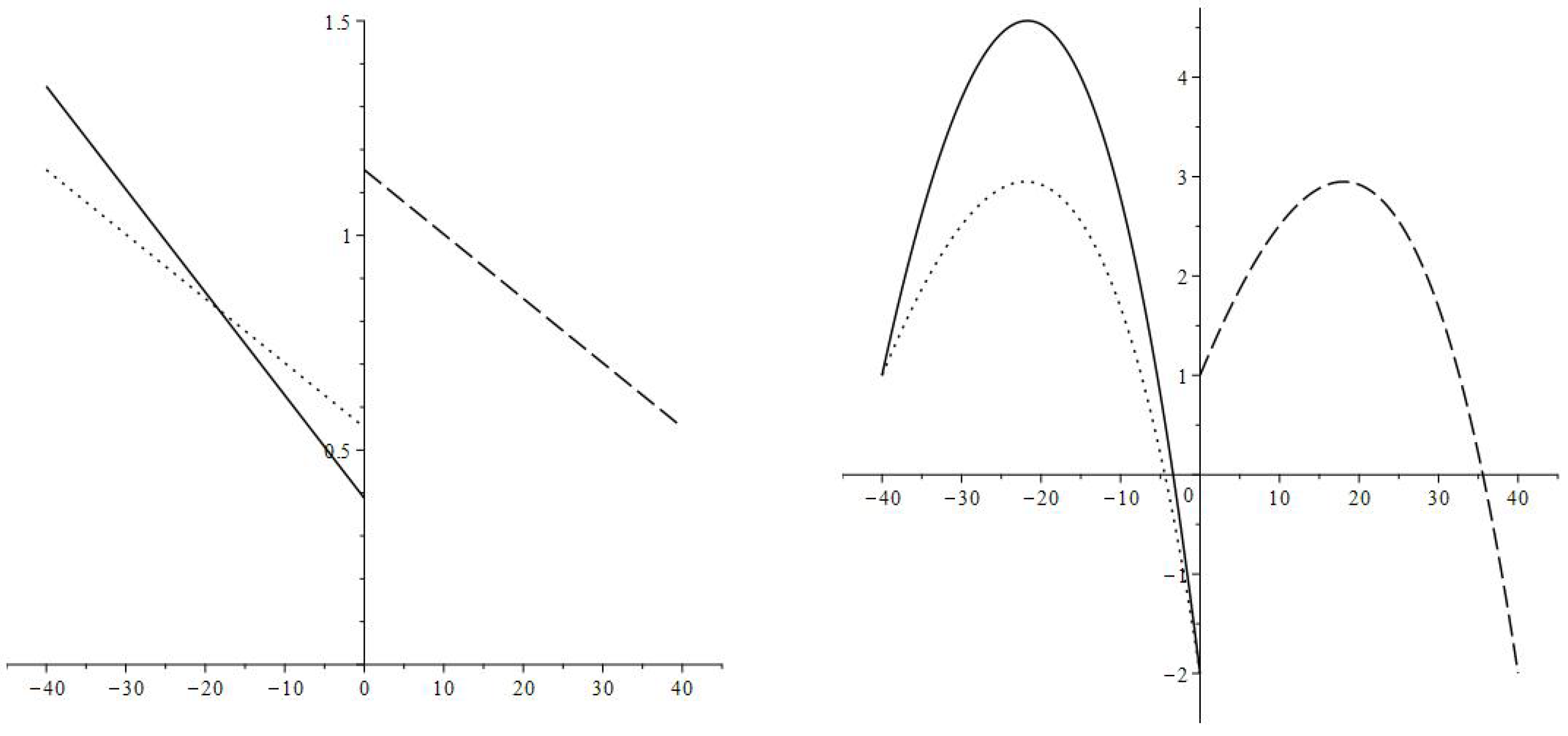
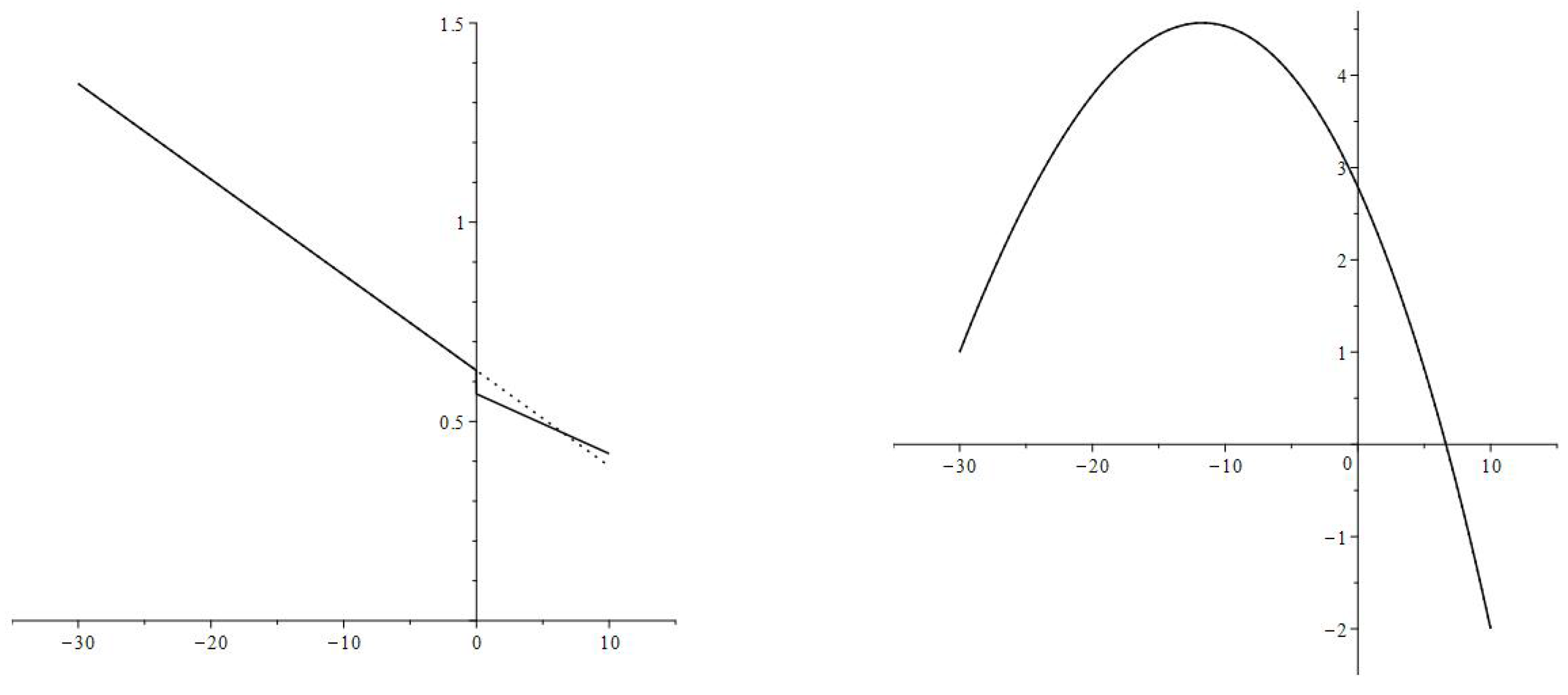
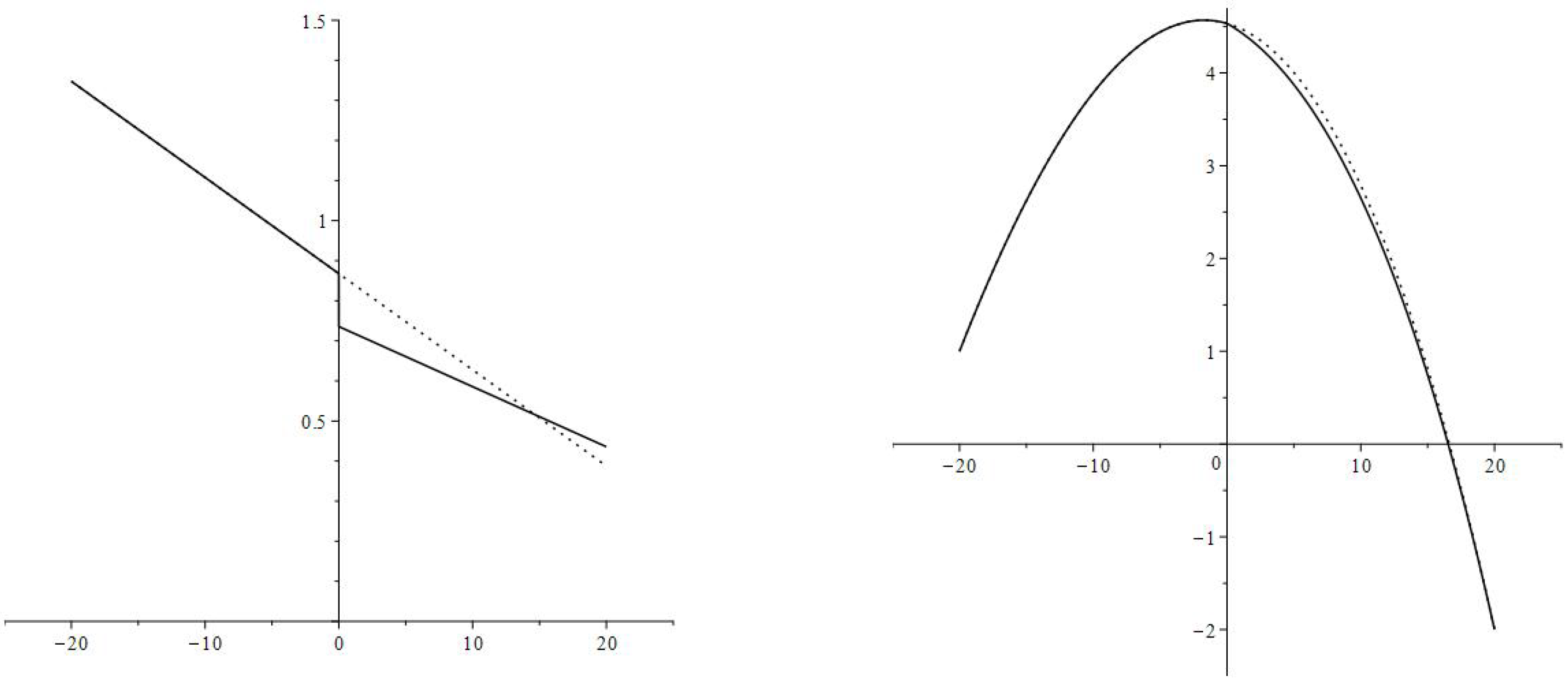
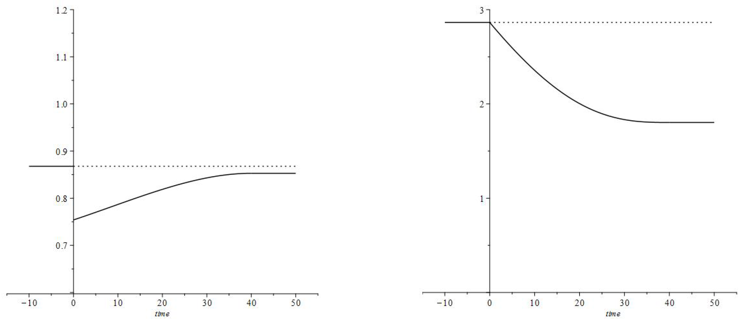
4.1. Interest Rate Changes Modeling

First, we discuss the effect of the interest rate change for particular age groups, described in Section 3.1. Then, we consider the averaged results, described in Section 3.3.

4.1.1. An Interest Rate Decrease

For the analysis of the effect of an interest rate decrease, we take the following parameters:

$$\begin{array}{c}T=40,w=1,K^0=1,K^T=-2,\hfill \\ r_0=0.04,{\delta }_0=0.055,r_1=0.02,{\delta }_1=0.044\hfill \end{array}$$

(42)

for the model described in the previous sections. Nonzero values $K^0$ and $K^T$ are chosen to consider the general case of the boundary conditions. The initial discount rate ${\delta }_0=0.055$ is chosen to fit the calibration condition $\max K=3w$, i.e., according to relation (26) with $\beta =3$. The new value of the discount rate ${\delta }_1=0.044$ is obtained as average of the three values given by the three particular methods (33)–(35).

The results for particular age groups are given in Figure 4, Figure 5, Figure 6 and Figure 7. Figure 4 compares the consumption pattern and the corresponding loan value dynamics before (for $t_0=-T$, $r=r_0$, $\delta ={\delta }_0$) and after (for $t_0=0$, $r=r_1$, $\delta ={\delta }_1$) the transition caused by the interest rate change. The slope of the consumption rate becomes steeper, indicating an increase of borrowing against the future earnings for the lower interest rate $r_1$. The greater values of the loan show the same.

Figure 5, Figure 6 and Figure 7 show the evolution of the consumption rate and borrowing pattern for three particular age groups: $t_0=-30$, $t_0=-20$ and $t_0=-10$. Comparison of the figures shows a minimal change (almost no change of the borrowing) for $t_0=-30$, a noticeable change for $t_0=-20$ and a substantial change for $t_0=-10$. It is reasonable to expect that the earlier (during the working life) the change in the interest rate takes place, the more substantial an effect on consumption and borrowing behavior it will have.

The averaged results are given in Figure 8. We observe that the consumption rate jumps by about 10% from $\overline{C}\left(0_{-}\right)={\overline{C}}_0$ to $\overline{C}\left(0_{+}\right)={\overline{C}}_1\left(0\right)$ at the moment of the interest rate change. Then, it decreases to the value $\overline{C}\left(T\right)={\overline{C}}_2$, ${\overline{C}}_2>{\overline{C}}_0$. During the transition the average loan value is substantially increased from $\overline{K}\left(0\right)={\overline{K}}_0$ to $\overline{K}\left(T\right)={\overline{K}}_2$.

It is important to stress that the consumption rate reaches its maximal value right after the interest rate change. This confirms that the decrease in interest rates can be an efficient tool to support consumption in times of recession or economic crisis. We observe that the optimal consumption rates for the individual age groups and the average consumption rate are discontinuous at the moment of the interest rate change: they have jump increases. Of course, different age groups respond differently to the interest rate change.

4.1.2. An Interest Rate Increase

Though the focus of this paper is on the interest rate decrease, for completeness of the discussion, we also provide a converse change of the interest rate. We use the same parameters as in the previous subsection and just interchange the values r and $\delta$ before and after the change, i.e., we analyze the effect of an interest rate increase using the parameters:

$$\begin{array}{c}T=40,w=1,K^0=1,K^T=-2,\hfill \\ r_0=0.02,{\delta }_0=0.044,r_1=0.04,{\delta }_1=0.055.\hfill \end{array}$$

(43)

for the model described in Section 2 and Section 3. The results are presented in Figure 9, Figure 10, Figure 11, Figure 12 and Figure 13. The changes are converse to those in the case of the interest rate decrease: an increase in the interest rate leads to an immediate jump decrease in the consumption rate, as shown in Figure 13. As time passes, the consumption rate increases to the value corresponding to the new interest rate. At the same time, the loan value decreases to the value corresponding to the new interest rate. As was observed in the previous subsection, the earlier in the life cycle the change happens, the more substantial an impact it has.

It should be noted that, in reality, it might be more challenging to reduce the debt load in the case of the interest rate increase than to increase borrowing in the case of the interest rate decrease. Therefore the simulation results of this subsection should be considered with some caution. Without a loan decrease, one can expect a more substantial decrease in the consumption rate.

4.2. Different Values of the New Interest Rate

Now we consider how the changes in the consumption and loan depend on the new interest rate $r_1$. We keep parameters,

$$T=40,w=1,r_0=0.04,{\delta }_0=0.055,$$

(44)

and remove the starting and final borrowing/saving

$$K^0=K^T=0$$

(45)

to make the discussion more universal.

First, we compute the values ${\delta }_1\left(r_1\right)$ provided by the methods (33)–(35). Figure 14 presents the simulation results. It shows that, for sufficiently large values of $r_1$ (roughly for $r_1\ge 0.03$), all three methods provide close values. However, for small values $r_1$, the methods differ. The approach based on the loan payment (35) does not work here. At the same time, the other two methods remain similar. The method based on the maximal loan value and the loan payment (33) seems the most reasonable.

According to Fortune and Ortmeyer (1985), the discount rate can be described as a constant plus the interest rate. For $r_1\ge 0.03$, all three methods seem to correspond to this statement. The phenomenon of low interest rates is recent and what happens to the discount rate in this case is much less understood.

Figure 15 and Figure 16 show the immediate change in the average consumption rate,

$$\frac{\overline{C}\left(0_{+}\right)-\overline{C}\left(0_{-}\right)}{\overline{C}\left(0_{-}\right)}=\frac{{\overline{C}}_1\left(0\right)-{\overline{C}}_0}{{\overline{C}}_0}$$

(46)

(at the moment of the interest rate change), and the final change in the average consumption rate,

$$\frac{\overline{C}\left(T\right)-\overline{C}\left(0_{-}\right)}{\overline{C}\left(0_{-}\right)}=\frac{{\overline{C}}_2-{\overline{C}}_0}{{\overline{C}}_0},$$

(47)

for different values $r_1$. Figures also provide the final change of the average loan,

$$\frac{\overline{K}\left(T\right)-\overline{K}\left(0\right)}{\overline{K}\left(0\right)}=\frac{{\overline{K}}_2-{\overline{K}}_0}{{\overline{K}}_0},$$

(48)

for different values $r_1$. We recall that there is no immediate change to the loan value: it is continuous. As can be expected, a decrease (an increase) in the interest rate leads to a greater (smaller) average consumption rate in the short run and final average loan values. The final average consumption rate is also greater (smaller). The figures correspond to two methods of ${\delta }_1\left(r_1\right)$ determination: (33) and (34). The second method gives more significant changes for both the consumption rates and the loan values.

5. Discussion of the Computational Results

We considered the effect of interest rate changes on household consumption and borrowing behavior. The primary motivation is to understand the stimulating effect of the interest rate decrease. The analysis is based on a simple model for particular age groups called the basic model. The results obtained for different age groups shape aggregate consumption. The debt load is also considered in the model.

It is assumed that the other factors are adjusted to the changes in the consumption rate (it can be expected that, in reality the other factors would diminish the effect of the interest rate changes on consumption).

The suggested approach is based on the following building elements:

• A simple basic model, which describes the consumption pattern of a household representing a specific age group. At this stage, the interest rate is constant;
• Incorporation of interest rate changes into the basics model as a parameter change. This change of the parameters affects the control problem system of Equations (10a)–(10c) The two cases of this system (before and after the interest rate change) are connected by the continuity of the loan value and by a relation determining the new value of the discount rate. The consumption rate is discontinuous at the moment of the interest rate change;
• The results concerning the consumption rates and the loan values for different age groups derive the aggregate values.

Such age-structured models seem appropriate for household consumption and borrowing decisions—households plan over a long (but finite) horizon. Some simplifying assumptions allow a partially analytical treatment of the model.

Numerical simulation was employed to understand the transition coursed by an interest rate change. Since no real data were used, the obtained results are qualitative. The numerical simulation in the previous section provides the following results. (To be specific, we consider a decrease in the interest rate.)

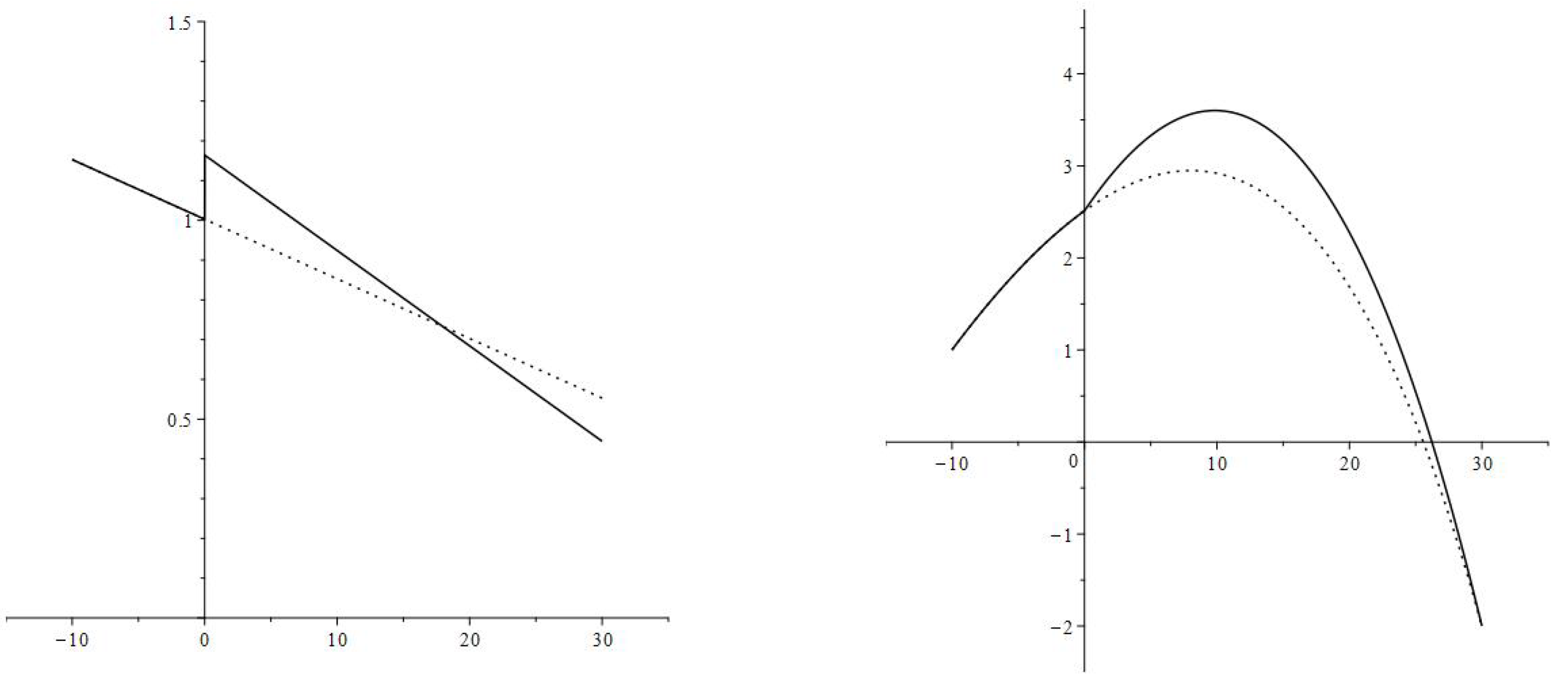
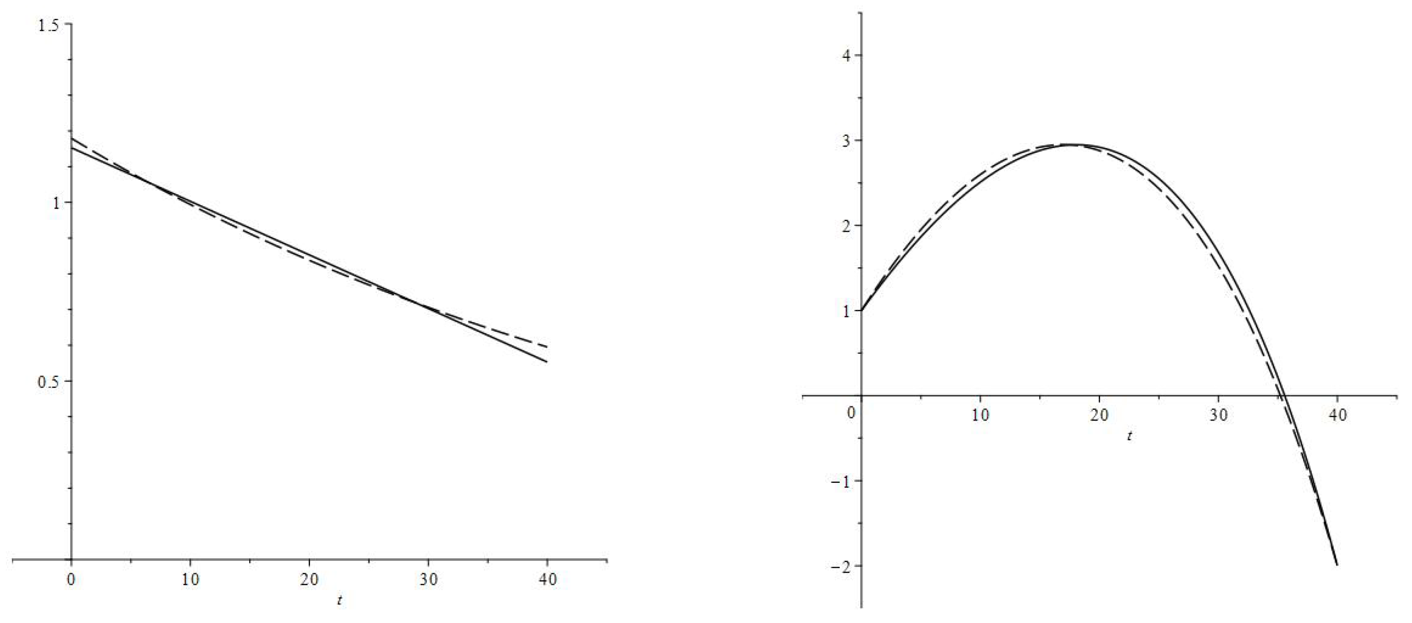
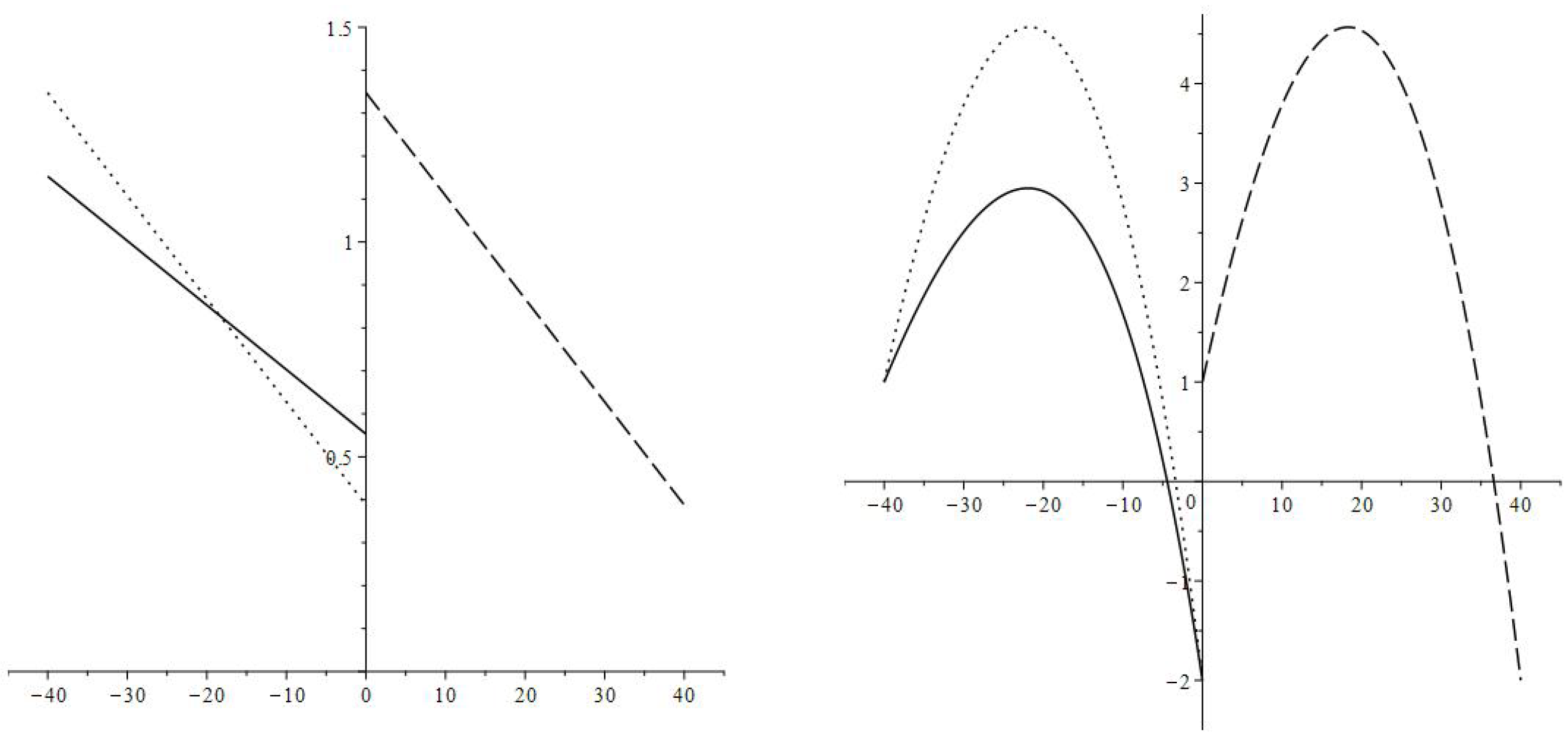
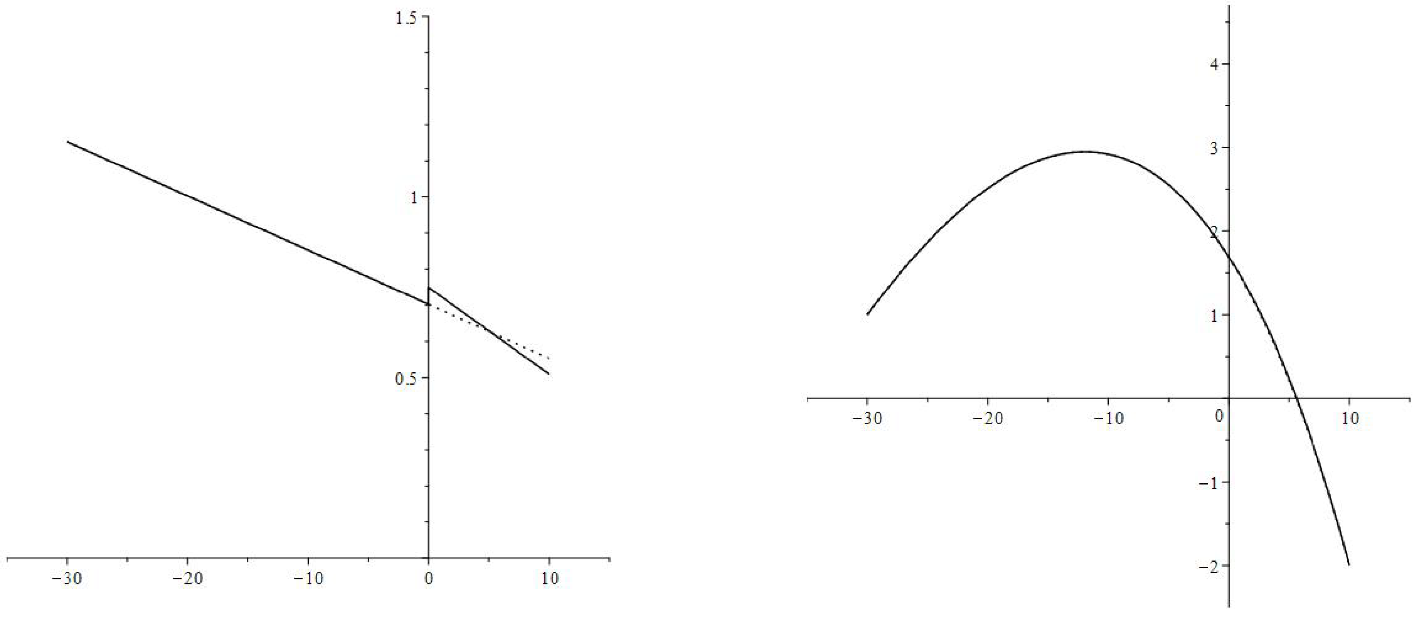
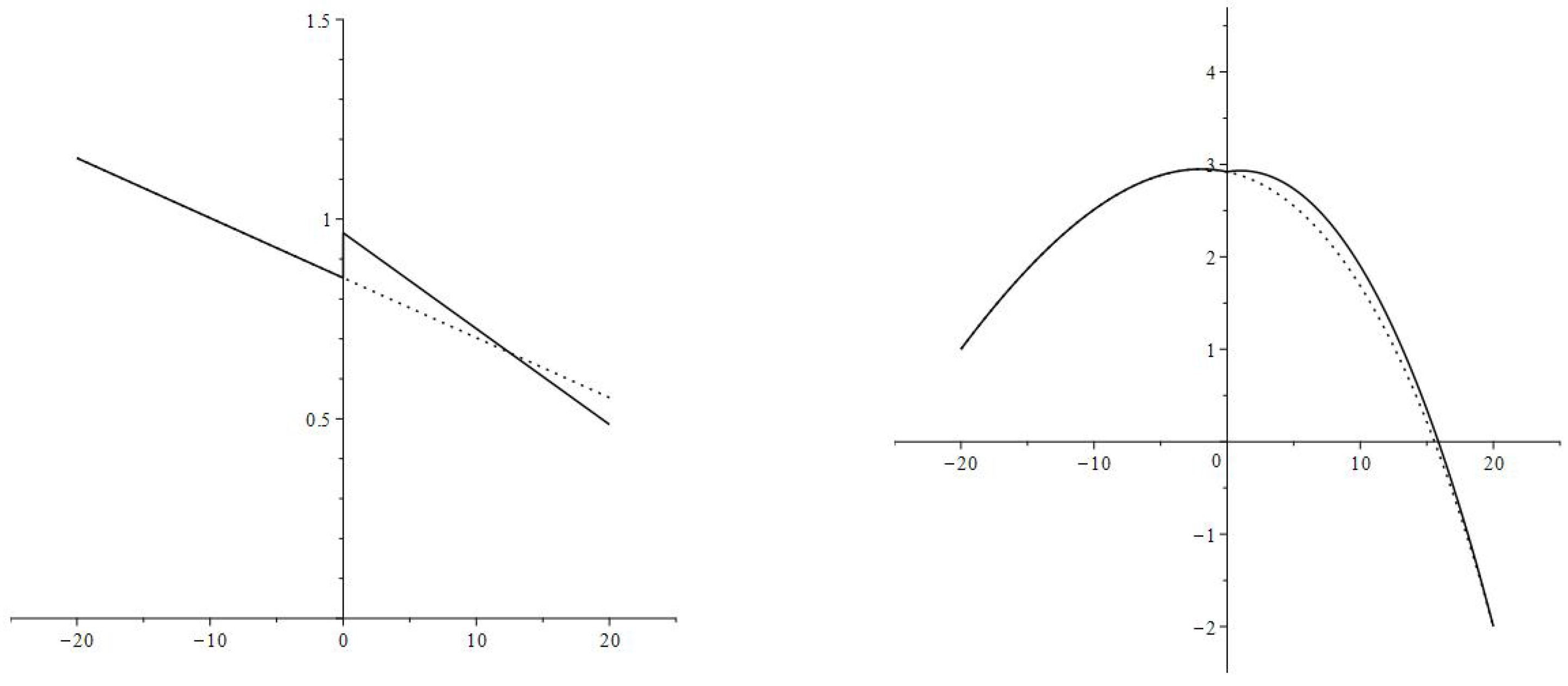
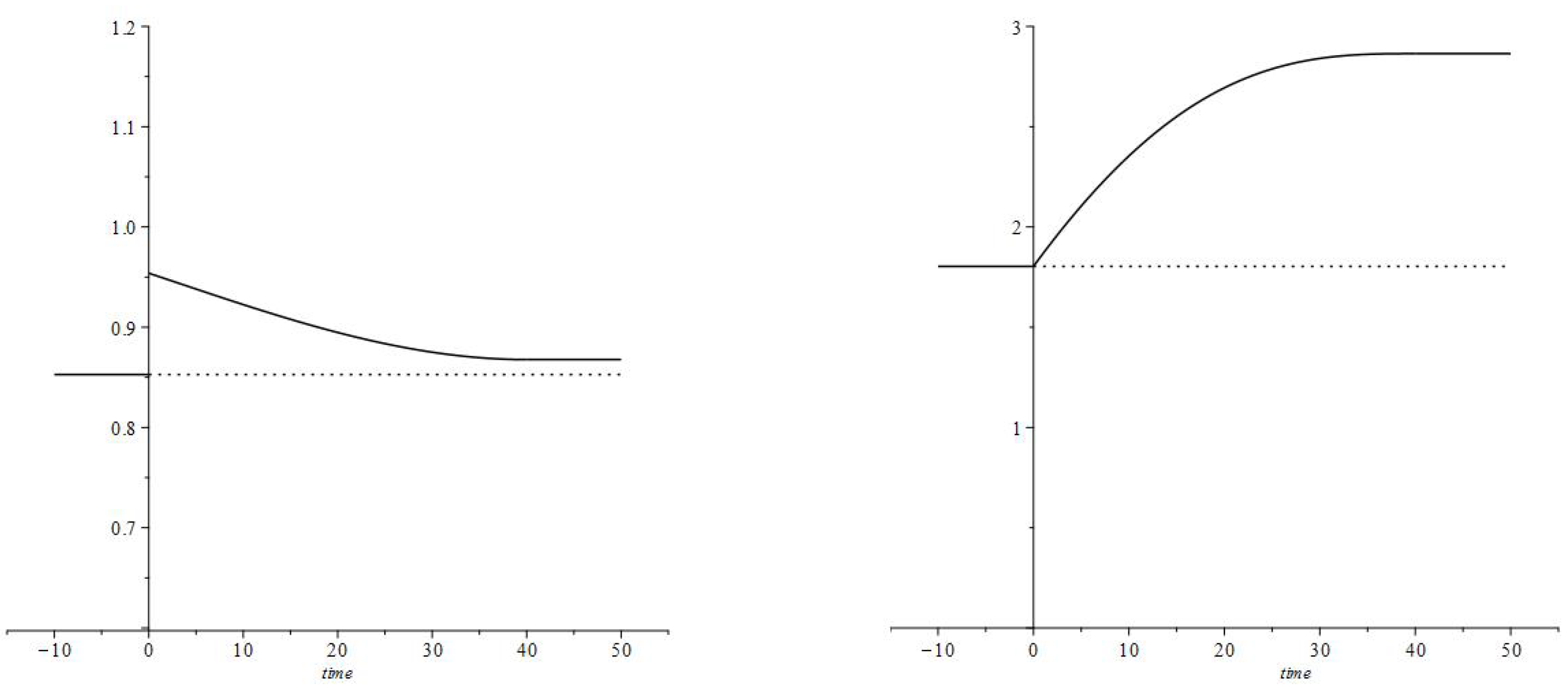
• The increase in consumption rate is most substantial right after the interest rate decrease. The consumption rates for individual age groups and the aggregate consumption rate have jump increases.
• After the immediate jump increase the average consumption rate decreases to the value corresponding to the new interest rate and discount factor (parameters $r_1$ and ${\delta }_1$). During the transition, the consumption rate is greater then upon the completion of the transition,

  $${\overline{C}}_1\left(t\right)>{\overline{C}}_1\left(T\right)={\overline{C}}_2,0<t<T,$$

  and ${\overline{C}}_1\left(t\right)$ is decreasing. In the numerical example, the new consumption rate (the consumption rate upon completion of the transition) is greater than the original consumption rate

  $${\overline{C}}_2>{\overline{C}}_0.$$
• High values of the consumption rate during the transition are achieved by an increase in the debt load:

  $${\overline{K}}_0={\overline{K}}_1\left(0\right)<{\overline{K}}_1\left(t\right)<{\overline{K}}_1\left(T\right)={\overline{K}}_2,0<t<T,$$

  (49)

  and ${\overline{K}}_1\left(t\right)$ is increasing.

There is an inverse relationship between the change in the interest rate and the change in the consumption rate. In the case of the interest rate increase, the average consumption rate has a jump decrease at the moment of the interest rate change and then shows a smooth increase in the final value. At the same time, the average loan gradually decreases to the final value.

Particular remarks should be made about the practice of interest rate reductions and low interest rates, as well as potential low interest rate increases. It should be noted that interest rate decreases are used for economic stimulation in times of recession or economic crisis. However, if used excessively, they can undermine sustainable economic and technological development.

Several concerns, as well as negative effects related to low values of the interest rates, were recently reported in the literature. They are mainly related to the efficiency of macroeconomic policy. Low interest rates can lead to record high public and private debt that presents a fragile balance with high costs of debt Rogoff (2020). It gives rise to the question: What is a safe level of public debt when interest rates are low Blanchard (2019)? It is natural to expect consumption to decrease in case of the interest rate increase Gerdrup and Torstensen (2018).

Low level interest rates make monetary policy less effective in stimulating bank lending growth Borio (2017). In a particular empirical study for Japan Iwata and Wu (2006) it was found that the effectiveness of monetary policy is lower when interest rates are close to zero. A rise in the interest rate can have an indirect effect on the deterioration of the property market Navarro and de Frutos (2012), including the growth of housing wealth and the growth rate of housing prices.

Overall, decreasing interest rates and the increasing role of credit have had both positive and negative consequences. On the one hand, they have made it easier for people to finance essential purchases, contributing to economic growth. On the other hand, they have also led to increased levels of debt, which can be difficult for some people to manage.

6. Concluding Remarks

The present paper suggests a theoretical model for the effect of interest rate changes on household consumption. Age-structured modeling was used to understand how changes in interest rates affect consumption behavior over different age groups. Younger individuals are more sensitive to changes in interest rates because they have more time than older individuals, while older individuals are less sensitive because they have less time to benefit from changes in interest rates. Consumption behavior of the particular age groups was described by methods of optimal control theory. The dependence of the subjective rate for discount $\delta$ on the interest rate r stands as a challenging issue of the present approach: there are too few empirical studies of this dependence.

It is worth mentioning that several simplifying assumptions, which were made to achieve analytical tractability, can be reconsidered to improve modeling. Probably the most significant correction can come from a better presentation of the income profile and the corresponding profile of the consumption pattern during the life cycle. Income $w(t,t_0)$ has an inverted U-shape (also called hump shape) and declines at retirement Attanasio and Weber (2010); Browning and Crossley (2001). It affects the consumption profile because consumption follows the changes in income.

Modeling intertemporal preferences can benefit from using a nonconstant discount factor $\delta$. The constant discount factor is standard in the economic literature. The nonconstant factor can take into account the evolution of individual needs. A recent study Kureishi et al. (2021) suggests that the discount rate decreases with age and the decline is linear over the life cycle.

There are different directions for future work. For real-life modeling, it is necessary to go beyond a single change of interest rates. It is possible to extend the approach presented in this paper to model gradual changes in interest rates. Such gradual changes can be approximated as sequences of jump changes from one value to another. Each particular change can be treated as the paper suggests.

Many other factors such as inflation, taxes, changes to higher economic and technological development paths, expectations about the future, etc., can also be included. It is particularly relevant to analyze household investments and different interest rates for borrowers and savers. This would require the application of more comprehensive models Acemoglu (2008); Alogoskoufis (2019); Greiner and Fincke (2015); Novales et al. (2014).

References

1. Acemoglu, Daron. 2008. Introduction to Modern Economic Growth. Princeton: Princeton University Press. [Google Scholar]
2. Alogoskoufis, George. 2019. Dynamic Macroeconomics. Cambridge: The MIT Press. [Google Scholar]
3. Alp, Esra, and Ünal Seven. 2019. The dynamics of household final consumption: The role of wealth channel. Central Bank Review 19: 21–32. [Google Scholar] [CrossRef]
4. Ando, Albert, and Franco Modigliani. 1963. The life cycle hypothesis of saving: Aggregate implications and tests. American Economic Review 53: 55–84. [Google Scholar]
5. Attanasio, Orazio P., and Guglielmo Weber. 2010. Consumption and saving: Models of intertemporal allocation and their implications for public policy. Journal of Economic Literature 48: 693–751. [Google Scholar] [CrossRef] [Green Version]
6. Barba, Aldo, and Massimo Pivetti. 2009. Rising household debt: Its causes and macroeconomic implications—A long-period analysis. Cambridge Journal of Economics 33: 113–37. [Google Scholar] [CrossRef] [Green Version]
7. Blanchard, Olivier. 2019. Public debt and low interest rates. American Economic Review 109: 1197–229. [Google Scholar] [CrossRef] [Green Version]
8. Borio, Claudio. 2017. Monetary policy and bank lending in a low interest rate environment: Diminishing effectiveness? Journal of Macroeconomics 54: 1339–51. [Google Scholar] [CrossRef] [Green Version]
9. Browning, Martin, and Thomas F. Crossley. 2001. The life-cycle model of consumption and saving. Journal of Economic Perspectives 15: 3–22. [Google Scholar] [CrossRef] [Green Version]
10. Caputo, Michael R. 2005. Foundations of Dynamic Economic Analysis: Optimal Control Theory and Applications. Cambridge: Cambridge University Press. [Google Scholar]
11. Carlino, Gerald A. 1982. Interest rate effects and intertemporal consumption. Journal of Monetary Economics 9: 223–34. [Google Scholar] [CrossRef]
12. Carroll, Christopher D. 1994. How does future income affect current consumption? Quarterly Journal of Economics 109: 111–47. [Google Scholar] [CrossRef] [Green Version]
13. Christen, Markus, and Ruskin M. Morgan. 2005. Keeping up with the Joneses: Analyzing the effect of income inequality on consumer borrowing. Quantitative Marketing and Economics 3: 145–73. [Google Scholar] [CrossRef]
14. Cloyne, James, Clodomiro Ferreira, and Paolo Surico. 2020. Monetary policy when households have debt: New evidence on the transmission mechanism. Review of Economic Studies 87: 102–29. [Google Scholar] [CrossRef]
15. Coskun, Yener, Nicholas Apergis, and Esra Alp Coskun. 2022. Nonlinear responses of consumption to wealth, income, and interest rate shocks. Empirical Economics 63: 1293–335. [Google Scholar] [CrossRef] [PubMed]
16. Di Maggio, Marco, Amir Kermani, Benjamin J. Keys, Tomasz Piskorski, Rodney Ramcharan, Amit Seru, and Vincent Yao. 2017. Interest rate pass-through: Mortgage rates, household consumption, and voluntary deleveraging. American Economic Review 107: 3350–588. [Google Scholar] [CrossRef] [Green Version]
17. Friedman, Milton. 1957. A Theory of the Consumption Function. Princeton: Princeton University Press. [Google Scholar]
18. Fortune, Peter, and David L. Ortmeyer. 1985. The roles of relative prices, interest rates, and bequests in the consumption function. Journal of Macroeconomics 7: 381–400. [Google Scholar] [CrossRef]
19. Gerdrup, Karsten R., and Kjersti Næss Torstensen. 2018. The effect of higher interest rates on household disposable income and consumption—A static analysis of the cash-flow channel. Norges Bank, Staff Memo 3. Available online: https://www.norges-bank.no/contentassets/acc6e77108104207bf2d4c8d44c48816/staff_memo_3_2018_eng.pdf?v=04/25/2018122116&ft=.pdf (accessed on 16 August 2021).
20. Gourinchas, Pierre-Olivier, and Jonathan A. Parker. 2002. Consumption over the life cycle. Econometrica 70: 47–89. [Google Scholar] [CrossRef] [Green Version]
21. Greiner, Alfred, and Bettina Fincke. 2015. Public Debt, Sustainability and Economic Growth. Theory and Empirics. Berlin/Heidelberg: Springer International Publishing. [Google Scholar]
22. Gylfason, Thorvaldur. 1981. Interest Rates, Inflation, and the Aggregate Consumption Function. The Review of Economics and Statistics 63: 233–45. [Google Scholar] [CrossRef]
23. Hertwich, Edgar G. 2005. Life cycle approaches to sustainable consumption: A critical review. Environmental Science and Technology 39: 4673–84. [Google Scholar] [CrossRef]
24. Iwata, Shigeru, and Shu Wu. 2006. Estimating monetary policy effects when interest rates are close to zero. Journal of Monetary Economics 53: 1395–408. [Google Scholar] [CrossRef]
25. Johnston, Alison, Gregory W. Fuller, and Aidan Regan. 2021. It takes two to tango: Mortgage markets, labor markets and rising household debt in Europe. Review of International Political Economy 28: 843–73. [Google Scholar] [CrossRef] [Green Version]
26. Kamien, Morton I., and Nancy Lou Schwartz. 2012. Dynamic Optimization, Second Edition: The Calculus of Variations and Optimal Control in Economics and Management. Dover Books on Mathematics. Chelmsford: Courier Corporation. [Google Scholar]
27. Kapeller, Jakob, and Bernhard Schutz. 2014. Debt, boom, bust: A theory of Minsky-Veblen cycles. Journal of Post Keynesian Economics 36: 781–814. [Google Scholar] [CrossRef] [Green Version]
28. Kaplan, Greg, and Giovanni L. Violante. 2014. A model of the consumption response to fiscal stimulus payments. Econometrica 82: 1199–239. [Google Scholar]
29. Keynes, John Maynard. 1936. The General Theory of Employment, Interest and Money. London: Macmillan. [Google Scholar]
30. Kureishi, Wataru, Hannah Paule-Paludkiewicz, Hitoshi Tsujiyama, and Midori Wakabayashi. 2021. Time preferences over the life cycle and household saving puzzles. Journal of Monetary Economics 124: 123–39. [Google Scholar] [CrossRef]
31. Leung, Siu Fai. 2000. Why Do Some Households Save So Little? A Rational Explanation. Review of Economic Dynamics 3: 771–800. [Google Scholar] [CrossRef] [Green Version]
32. Mian, Atif, Amir Sufi, and Emil Verner. 2017. Household debt and business cycles worldwide. Quarterly Journal of Economics 132: 1755–817. [Google Scholar] [CrossRef] [Green Version]
33. Modigliani, Franco, and Richard Brumberg. 1954. Utility analysis and the consumption function: An interpretation of cross-section data. In Post-Keynesian Economics. Edited by Kenneth K. Kurihara. New Brunswick: Rutgers University Press, pp. 388–436. [Google Scholar]
34. Navarro, Manuel León, and Rafael Flores de Frutos. 2012. Consumption and housing wealth breakdown of the effect of a rise in interest rates. Applied Economics 44: 2091–110. [Google Scholar] [CrossRef]
35. Navarro, Manuel León, and Rafael Flores de Frutos. 2015. Residential versus financial wealth effects on consumption from a shock in interest rates. Economic Modelling 49: 81–90. [Google Scholar] [CrossRef]
36. Novales, Alfonso, Esther Fernández, and Jesús Ruíz. 2014. Economic Growth. Theory and Numerical Solution Methods. Berlin/Heidelberg: Springer. [Google Scholar]
37. Pontryagin, Lev S., Vladimir G. Boltyanskii, Revaz V. Gamkrelidze, and Evgenii F. Mishechenko. 1962. The Mathematical Theory of Optimal Processes. New York and London: John Wiley & Sons. [Google Scholar]
38. Rogoff, Kenneth. 2020. Falling real interest rates, rising debt: A free lunch? Journal of Policy Modeling 42: 778–90. [Google Scholar] [CrossRef]
39. Sierstad, Atle, and Knut Sydsaeter. 1987. Optimal Control Theory with Economic Applications. Amsterdam: North-Holland. [Google Scholar]
40. Tauheed, Linwood, and L. Randall Wray. 2006. System dynamics of interest rate effects on aggregate demand. In Money, Financial Instability and Stabilization Policy. Edited by L. Randall Wray and Mathew Forstater. Cheltenham: Edward Elgar Pub, pp. 37–57. [Google Scholar]
41. Taylor, Mark P. 1999. Real interest rates and macroeconomic activity. Oxford Review of Economic Policy 15: 95–113. [Google Scholar] [CrossRef]
42. Van Tran, Nguyen. 2022. Understanding Household Consumption Behaviour: What do we Learn from a Developing Country? B.E. Journal of Economic Analysis and Policy 22: 801–58. [Google Scholar] [CrossRef]
43. Weber, Thomas A. 2011. Optimal Control Theory with Applications in Economics. Cambridge: The MIT Press. [Google Scholar]
44. Wolff, Edward N. 2011. Recent trends in household wealth in the U.S.: Rising debt and the middle class squeeze (Book Chapter). In Economics of Wealth in the 21st Century. Edited by Jason M. Gonzalez. New York: Nova Science Publishers, Inc., pp. 1–41. [Google Scholar]
Figure 1. US Households and Nonprofit Organizations; Consumer Credit; 1980–2021. Source: FRED.
Economies 11 00023 g001
Figure 2. Discount Rate for the United States 1980–2021. Source: FRED.
Economies 11 00023 g002
Figure 3. Ten-year US Government Bond Yields 1980–2021. Source: FRED.
Economies 11 00023 g003
Figure 4. The interest rate decrease scenario. The consumption rate (left) and the loan value (right): the initial pattern for the interval [ 40 , 0 ] , i.e., for age group t 0 = 40 , (solid line), the final pattern for the interval [ 0 , 40 ] , i.e., for age group t 0 = 0 , (dashed line) and the final pattern shifted to the initial interval (dotted line).
Economies 11 00023 g004
Figure 5. The interest rate decrease at t = 0 . The consumption rate (left) and the loan value (right) for the interval [ 30 , 10 ] , i.e., for age group t 0 = 30 . The dotted line shows how it would be without the change in the interest rate.
Economies 11 00023 g005
Figure 6. The interest rate decrease at t = 0 . The consumption rate (left) and the loan value (right) for the interval [ 20 , 20 ] , i.e., for age group t 0 = 20 . The dotted line shows how it would be without the change in the interest rate.
Economies 11 00023 g006
Figure 7. The interest rate decrease at t = 0 . The consumption rate (left) and the loan value (right) for the interval [ 10 , 30 ] , i.e., for age group t 0 = 10 . The dotted line shows how it would be without the change in the interest rate.
Economies 11 00023 g007
Figure 8. The transition for the interest rate decrease at t = 0 . The average consumption rate (left) and the average loan value (right) for parameters (42). The transition happens on the interval [ 0 , 40 ] . The dotted line shows how it would be without the change in the interest rate.
Economies 11 00023 g008
Figure 9. The interest rate increase scenario. The consumption rate (left) and the loan value (right): the initial pattern for the interval [ 40 , 0 ] , i.e., for age group t 0 = 40 , (solid line), the final pattern for the interval [ 0 , 40 ] , i.e., for age group t 0 = 0 , (dashed line) and the final pattern shifted to the initial interval (dotted line).
Economies 11 00023 g009
Figure 10. The interest rate increase at t = 0 . The consumption rate (left) and the loan value (right) for the interval [ 30 , 10 ] , i.e., for age group t 0 = 30 . The dotted line shows how it would be without the change in the interest rate.
Economies 11 00023 g010
Figure 11. The interest rate increase at t = 0 . The consumption rate (left) and the loan value (right) for the interval [ 20 , 20 ] , i.e., for age group t 0 = 20 . The dotted line shows how it would be without the change in the interest rate.
Economies 11 00023 g011
Figure 12. The interest rate increase at t = 0 . The consumption rate (left) and the loan value (right) for the interval [ 10 , 30 ] , i.e., for age group t 0 = 10 . The dotted line shows how it would be without the change in the interest rate.
Economies 11 00023 g012
Figure 13. The transition for the interest rate increase at t = 0 . The average consumption rate (left) and the average loan value (right) for parameters (43). The transition happens on the interval [ 0 , 40 ] . The dotted line shows how it would be without the change in the interest rate.
Economies 11 00023 g013
Figure 14. Determination of δ 1 ( r 1 ) for parameters (44) and (45). Three approaches are given: the method based on the maximal loan value and the loan payment (solid line); the method based on the average loan value and the loan payment (dashed line); and the method based on the loan payment (dotted line).
Economies 11 00023 g014
Figure 15. Left plots: The immediate change of the average consumption rate, ( C ¯ ( 0 + ) C ¯ 0 ) / C ¯ 0 , in percent (solid line) and the final change in the average consumption rate, ( C ¯ 2 C ¯ 0 ) / C ¯ 0 , in percent (dashed line). Right plot: The final change of the average loan value, ( K ¯ 2 K ¯ 0 ) / K ¯ 0 , in percent. The plots use the determination of δ 1 based on the maximal loan value and the loan payment.
Economies 11 00023 g015
Figure 16. Left plots: The immediate change of the average consumption rate, ( C ¯ ( 0 + ) C ¯ 0 ) / C ¯ 0 , in percent (solid line) and the final change in the average consumption rate, ( C ¯ 2 C ¯ 0 ) / C ¯ 0 , in percent (dashed line). Right plot: The final change of the average loan value, ( K ¯ 2 K ¯ 0 ) / K ¯ 0 , in percent. The plots use the determination of δ 1 based on the average loan value and the loan payment.
Economies 11 00023 g016
Disclaimer/Publisher’s Note: The statements, opinions and data contained in all publications are solely those of the individual author(s) and contributor(s) and not of MDPI and/or the editor(s). MDPI and/or the editor(s) disclaim responsibility for any injury to people or property resulting from any ideas, methods, instructions or products referred to in the content.