Macroprudential and Monetary Policy Interactions and Coordination in South Africa: Evidence from Business and Financial Cycle Synchronisation

Abstract

The article reports on the interactions and possibility of coordination between macroprudential and monetary policies in South Africa, based on business and financial cycles synchronisation. To this end, relying on financial and economic time series indicators spanning the period 2000M01–2018M12, a two-step Markov switching dynamic factor model was adopted for the measurement of composite indices, while both the dynamic conditional correlations and asymmetric generalised dynamic conditional correlations models were adopted for synchronisation analysis, together with the Metcalfe scale of coordination. The empirical evidence obtained is such that, under conditions of financial and real economic stress in South Africa, when there is crisis management rather than crisis prevention, macroprudential policy and monetary policy decisions are complementary. Therefore, there will be limited/no need for coordination between the two policy decisions. However, under normal times when there is crisis prevention rather than management, macroprudential policy and monetary policy decisions are noncomplementary; hence, the greatest degree of coordination is warranted, even though it might not be easy. Therefore, we conclude that it is possible to the coordinate the conduct of macroprudential, and monetary policies based on the synchronicity of business and financial cycles.

1. Introduction

This article aims to explore the interactions between macroprudential and monetary policies in South Africa. Prior to the 2007–2009 global financial crises (GFCs), there was a near consensus among economists and policymakers that monetary policy (MP) should be set out to deliver price stability and microprudential (MiPP) regulation and supervision, to deliver financial stability. MP ought to respond to financial system developments insofar as they affect inflation (Frait et al. 2014; Malovana and Frait 2017). However, the severity of the 2007–2009 GFCs and their costs on the real economies of different nations proved that policymakers require a broader approach to safeguard the financial system. As a result, the call for regulatory frameworks that are macro-systemic risk dedicated, namely macroprudential policy (MaPP), was strengthened, where MaPP refers to “the tools utilised to target sources of risk of disruptions to the provision of key financial services that is caused by the impairment of all or parts of the financial system” (Malovana and Frait 2017, p. 2).

Presently, both MaPP and MP represents an integral part of the Central Banks’ policy framework with their distinct objectives and processes. In South Africa, in accordance with the Financial Sector Regulations Bill (FSR Bill), apart from its main objective of price stability, it is also the South African Reserve Bank’s (SARB) responsibility to monitor the South African financial system for potential systemic risks (South African Reserve Bank 2016). The SARB must take all rational steps to thwart systemic risk events and to mitigate the adverse effects of such events on financial stability through the application of MaPP toolkits of instruments. This means that the SARB is now an integrated monetary and supervisory authority, responsible for both the objectives of price and financial stability. To date, there exists a near consensus among economists and policy makers that monetary and macroprudential policy tools are not independent. MaPP, in pursuit of financial stability, may have implications for MP. Similarly, MP in pursuit of price stability may have implications for MaPP (Dunstan 2014).

Disagreement exists, however, on the analytical and policy approach taken to manage the existing interactions between the two main objectives of price and financial stability. There are three dominant strands of literature on the analyses of interactions between MaPP and MP (Malovaná et al. 2023). The first strand advocates for a clear separation of policy objectives, also referred to as the modified Jackson Hole consensus. The second strand acknowledges the different interactions between the two policy objectives and considers them inseparable; hence, coordination is considered mandatory. The last strand in the literature proposes taking risks to financial stability into account in MP conduct even if the current forecast indicates no risk to price stability. This is referred as the “lean against the wind consensus” (Malovaná et al. 2023).

To date, it is agreed that MaPP and MP both affect the functioning of the entire financial system and the economy. Therefore, it remains imperative that when designing and implementing the objectives of these two policies, central banks take into consideration how they interact and ensure they are coordinated; coordinated; this is in line with the second strand of the literature (Dunstan 2014; Frait et al. 2014). It is further agreed that conflict may arise between the two policies due to the need for them to work in opposite directions. Accordingly, conflict arises due to the time inconsistency associated with the conduct of MaPP and MP, as well as in situations where the economy is in different stages of business cycles (BCs) and financial cycles (FCs) (Malovana and Frait 2017; Malovaná et al. 2023). This has raised further disagreement on which policy option the central bank should favour in cases where there is conflict, with some advocating for MaPP to be temporarily favoured, while others advocate for MP to always be favoured. Nonetheless, according to the present literature (Dunstan 2014; Frait et al. 2014; Malovana and Frait 2017; Malovaná et al. 2023; Spencer 2014), the right policy mix partly depends on the interactions of two different cycles; the business cycle (BC) and the financial cycle (FC).

It is therefore necessary to analyse the interactions and coordination of MaPP and MP based on the interactions of BCs and FCs. While the interactions between BCs and FCs are the focal point of several studies in the present literature (Adrian et al. 2010; Billio and Petronevich 2017; Borio 2014a, 2014b; Borio et al. 2001; Cagliarini and Price 2017; Claessens et al. 2011, 2012; Leamer 2007; Rünstler and Vlekke 2015; Stock and Watson 2003), only a few studies have considered the extent to which BCs and FCs are synchronised (Akar 2016; Frait et al. 2014; Gökalp and Yu 2018; Malovana and Frait 2017; Sala-Rios et al. 2016; Spencer 2014; Tsiakas and Zhang 2023). These studies have established a strong link between BCs and FCs. Nevertheless, such findings were only for developed or a group of developed countries, whereas this is also an issue of vital importance for both policy and investment decision making. There are even fewer studies exploring the interactions between BCs and FCs with the intention of enhancing the understanding of MaPP and MP interactions and their possibility of coordination, concurrently.

In line with the cyclical component of systemic risks, the writers of the present article set out to examine the interactions and the possibility of coordination between MaPP and MP based on the synchronisation of BCs and FCs in South Africa. Explicitly, through the adoption of a two-step Markov switching dynamic factor model (MS-DFM) and real and financial time series data covering the period 2000M01–2018M12, the article develops a composite business cycle index and a composite financial cycle index as measures of the BC and the FC in South Africa. Further, through the adoption of a time-varying dynamic conditional correlations multivariate GARCH (DCC MGARCH) model, and an asymmetric generalised DCC MGARCH model, the article empirically investigates the synchronisation and degrees of synchronisation between BCs and FCs in South Africa. The article culminates by utilising the synchronisation knowledge obtained to provide new evidence on coordination and coordination degrees between MaPP and MP in South Africa.

2. Literature on Conceptual and Empirical Matters

Over time, there has been consensus between several economists and policy makers that macroprudential and monetary policy tools are not independent as they affect both the functioning of the entire economy and the credit conditions via their effect on asset prices, credit growth, and financial risk taking (Agénor et al. 2013; Malovana and Frait 2017; Smets 2018). Disagreement exists, however, on the analytical and policy approach taken to manage the existing interactions between the two main objectives of price and financial stability. There are three dominant strands of literature on the analyses of interactions between MaPP and MP as mentioned above. The first advocates for a clear separation of objectives. Explicitly, advocates of this view are of the belief that central banks should focus their attention on achieving price stability while MaPP measures should be assigned to achieve financial stability. They believe the two objectives are independent of each other (Malovaná et al. 2023).

The second strand of the literature and by far the most popular in recent literature considers price stability and financial stability to be strongly intertwined and inseparable, suggesting that policy coordination is desirable to achieve the best economic outcome. Macro-financial linkages, creating feedback loops between the real economy and the financial system, are at the core of this view (Dunstan 2014; Frait et al. 2014; Hollander and Van Lill 2019; Malovana and Frait 2017). The third and final strand of the literature focuses on taking risks to financial stability into account in MP conduct even if current forecasting indicates no risk to price stability. Advocates of this view acknowledge that macroprudential policy cannot fully address the existing or potential systemic risks while monetary policy can be effective in this pursuit (Malovaná et al. 2023).

According to the present literature (Dunstan 2014; Frait et al. 2014; Hollander and Van Lill 2019; Malovana and Frait 2017), it is clear that both MaPP and MP affect the functioning of the entire financial system and the economy. When configuring these two policies, central banks need to consider how they interact and ensure they are coordinated (Spencer 2014). The key idea is to attain the right policy mix and to ensure that the primary aims of the two policies are not adversely affected by too heavily diverting the attention of the policies towards secondary objectives, avoiding costs associated with the consequences of policy action or policy inaction (Hollander and Van Lill 2019). This is in line with the second strand of the literature which advocates for policy coordination between MaPP and MP.

However, while there is clearly a need to coordinate MaPP and MP conceptually, practically, such coordination remains a difficult task for almost all central banks (Hollander and Van Lill 2019). According to Malovana and Frait (2017), one of the main contributing factors to this coordination difficulty has been the limited understanding of the interactions between these two policies—so much so that it has strengthened the likelihood of failure to achieve the main policy objectives. Consequently, this has posed threats to the credibility of the institutions and hindered proper decision making about policy actions. This makes it necessary to study the interactions between MaPP and MP and their coordination concurrently. This is in line with the cyclical component of systemic risks as opposed to the structural component of systemic risks (Hodula et al. 2023).

According to Hodula et al. (2023), systemic risk possesses two components. The first is a cyclical component which is basically linked to the evolution of the financial cycle, its measurement, and its relationship with the real economy. The second is the structural component which has to do with the distribution of risk in the financial sector. Presently, it is noted that the current literature is seemingly skewed towards the cyclical risk component of systemic risk and tends to focus less on the structural component despite its importance. This is, however, to be expected, given the fact that the concepts themselves are still in their infant stages of development and several issues remain unresolved, thus requiring further focus. This is not to say that structural risks deserve to be ignored but to allude to the fact that more needs to be conducted to reach a point of agreement on the part of the interactions of the financial system and the real economy.

Presently, within the second strand of the literature and in line with the cyclical component of systemic risk, two literature strands remain relevant. The first strand of the literature comprises empirical work on the analysis of coordination and the optimal policy mix between MaPP and MP, mainly through the adoption of dynamic stochastic general equilibrium models (DSGE) (Agur 2019; Claessens 2013; Kokores 2015; Liu and Molise 2020; Pan and Zhang 2020; de Paoli and Paustian 2017; Smets 2018). However, these models remain highly stylised and abstract from several important economic linkages and transition mechanisms. As a result, they usually fail to fully capture the dynamics of monetary and financial conditions (Frait et al. 2014). Hence, these models are more useful when the focus is on the structural component of systemic risk. Apart from the criticisms of the DSGE models as above, such analyses are beyond the scope of this article.

The second strand of the literature postulates that the right policy mix between MaPP and MP is dependent on the interactions between two different cycles, namely, the business cycle and the financial cycle (Adrian and Liang 2016; Frait and Komárková 2010; Frait et al. 2014; Malovana and Frait 2017; Spencer 2014). There has been an enormous amount of interest in studying the interactions between BCs and FCs, with the sole purpose of disentangling the characteristic relations and stylised features of these cycles (Borio 2014b; Borio et al. 2001; Claessens et al. 2011; Claessens et al. 2012; Farrell and Kemp 2020). There has been a limited amount of effort devoted towards studying the interactions between BCs and FCs to enhance the understanding of the interactions between MaPP and MP and their coordination concurrently. This is especially true in developing or underdeveloped countries where such analyses are still at their infant stages of development.

Among the limited number of studies dedicated towards this largely unexplored avenue of research, one approach towards studying the interactions of BCs and FCs has been the examination of synchronisation and the extent of synchronisation between the two cycles. From two writers, Dunstan (2014) and Spencer (2014), a rule for analysing the interactions and coordination between MaPP and MP through the synchronisation of BCs and FCs was provided. Accordingly, when BCs and FCs are synchronised, MaPP and MP decisions will be complementary. Therefore, coordination will be simple, just requiring each policy setting to cater for the complementary effects of the other. At times, there will be limited or no need to coordinate the policy decisions. On the other hand, when BCs and FCs are not synchronised, MaPP and MP decisions are noncomplementary. Therefore, there will be a greater potential for conflict between the two policy decisions. The primary objectives of the two policies will need to be carefully balanced; hence, there will be the greatest need for coordination even though difficult (Dunstan 2014; Spencer 2014).

While the concepts of cyclical synchronisation and desynchronisation are not new in the macroeconomics literature, empirical work on these concepts has rather focussed on BCs synchronisation within and between countries, while others have focused on FCs synchronisation between and within countries (Ahmed et al. 2018; Artis et al. 2004; Comrey and Lee 2013; Gächter et al. 2012; Gogas and Kothroulas 2009; Kose et al. 2012; Mink et al. 2007; Nzimande and Ngalawa 2016; Savva et al. 2010). There exist only a few studies which are dedicated to the analysis of the synchronisation and desynchronisation of BCs and FCs simultaneously.

Among the few studies dedicated to the analysis of BCs and FCs synchronisation and desynchronisation, results have often remained diverse. While some have found BCs and FCs to be highly synchronised, others have found these cycles to be highly desynchronised (Akar 2016; Billio and Petronevich 2017; Choudhry et al. 2016; Gökalp and Yu 2018; Oman 2019; Sala-Rios et al. 2016). For example, estimating a dynamical influence Markov switching dynamic factor model on US data to study the intersections between BCs and FCs, Billio and Petronevich (2017) found that synchronisation differs with the differing regimes of interaction between the two cycles. Further, in Oman (2019), it was found that FCs are less synchronised compared to BCs, BC synchronisation increased while FC synchronisation decreased, and FC desynchronisation was more pronounced between high amplitude and low amplitude countries viz. Germany.

In contrast to the above studies, in Claessens et al. (2012), an extensive database covering 44 countries for the period 1960: Q1–2010: Q4 was adopted to study the synchronisation between BCs and FCs. The results obtained showed that there exists strong synchronicity between the different phases of BCs and FCs. In line with Claessens et al. (2012), in Akar (2016), the relationship and synchronicity between BCs and FCs in Turkey was investigated. Utilising quarterly data observed over the period 1998Q1 to 2014Q4, evidence of strong synchronisation between BCs and FCs was found. These results were confirmed in Gökalp and Yu (2018), who also showed that the two cycles are immensely synchronised in the Turkish economy.

The extensive ground of the literature as analysed above, points to different conclusions with regards to the synchronicity of BCs and FCs. However, none or very few neither of these studies have analysed the synchronicity between BCs and FCs, to enhance the understanding of the interactions between MaPP and MP, and their possibility of coordination, concurrently. As a result, the writers of the present article delve deep into the analyses of synchronicity between BCs and FCs, with the sole purpose of providing new evidence about the interactions of MaPP and MP policies in South Africa. To this end, the article relies on composite indices and various statistical methods viz: DCC and ADCC MGARCH, to carry out its objectives. This article is the first of its kind to examine the interactions between MaPP and MP and their coordination, based on the interactions between BCs and FCs.

3. Database and Methodology

3.1. Database and Data Modifications

An extensive database was constructed using monthly time series of financial and economic variables for South Africa, covering the period 2000M01 to 2018M12. While the literature has not yet reached a consensus on the time series indicators that should be utilised to measure FCs and BCs, in this article, Krznar and Matheson (2017), Chorafas (2015), Ma and Zhang (2016), among others, are followed to measure the CFCI. Furthermore, the recommendations of Doz and Petronevich (2016), Venter (2009), and Vermeulen, Bosch, Rossouw, and Joubert (Vermeulen et al. 2017), among others, are used to measure the CBCI. This research has adopted thirteen (13) monthly financial time series variables to measure the CFCI. Eighty (80) financial and real economic time series variables adopted by the SARB were carefully selected to measure the CBCI. The specific CFCI and CBCI variables, descriptions, and data sources are shown in

Table 1. CFCI variables, description, and sources.

Variable	Abreviation	Description	Source
Real Broad effective exchange rate	RBEER	RBEER is a measure of value of the currency against a weighted average of several foreign currencies divided by a price deflator or index of cost (Pineda et al. 2009).	South African Reserve Bank
House Prices	HP	HP is measured by the Residential Property Price Index showing indices of residential property prices over time.	Bank for International Settlements
All Share Price Index	ASP	ASP is the total share price for all share on the JSE.	South African Reserve Bank
Long-term Government bond yields	LTGBY	LTGBY represents long-term interest rates exceeding 10 years	South African Reserve Bank
10-year Government bond yields	GB10Y	GB10Y represents long-term interest rates equal to 10 years	South African Reserve Bank
5-year Government bond yields	GB5Y	GB5Y represents short-term interest rates less than 10 years	South African Reserve Bank
Total credit to the private Non-Financial sector	TCPFS	TCPFS is provided by domestic banks, all other sectors of the economy and non-residents.	OECD, Reserve Bank of St Louis
Nominal effective exchange rate	NEER	NEER is calculated as geometric weighted averages of bilateral exchange rates.	OECD, Reserve Bank of St Louis
Treasury Bill Rate	TBILL	TBILL is a short-term debt obligation of the central government	South African Reserve Bank
The three measures of money in South Africa	M1, M2 and M3	Narrow Measure, Intermediate measure, Broad measure	South African Reserve Bank
Interbank Lending rate	ILR	ILR is the rate charged on short-term loans between South African banks	OECD, Reserve Bank of St Louis

and

Table A1. CBCI Variables, Description and Sources.

List of Indicators Used to Describe Composite Business Cycle Index
SARB Selected Monthly release	WHOLESALE SALES
SARB Selected Monthly release	RETAIL SALES
SARB Selected Monthly release	NEW PASS VEHICLE
SARB Selected Monthly release	Real estate loans
SARB Selected Monthly release	IP-Total M
SARB Selected Monthly release	IP-food and beverages
SARB Selected Monthly release	IP-Raw Material
SARB Selected Monthly release	IP-textiles, Leather,
SARB Selected Monthly release	IP-wood and paper
SARB Selected Monthly release	IP-Equipment
SARB Selected Monthly release	IP-Durable Material
SARB Selected Monthly release	IP-Fuels
SARB Selected Monthly release	Building Plans Pd
SARB Selected Monthly release	Real Eff EX
SARB Selected Monthly release	M0
SARB Selected Monthly release	M1
SARB Selected Monthly release	M2
SARB Selected Monthly release	SA/ US dollar
SARB Selected Monthly release	SA/British pound
SARB Selected Monthly release	SA/Euro
SARB Selected Monthly release	SA/Japanese yen
SARB Selected Monthly release	Reserves of commercial Banks
SARB Selected Monthly release	Total Loans
SARB Selected Monthly release	Total Credit Ext
SARB Selected Monthly release	PPI-ALL GROUPS
SARB Selected Monthly release	PPI-INTERMEDIATE
SARB Selected Monthly release	PPI-CRUDE OILS
SARB Selected Monthly release	PPI-MANUFACTURING
SARB Selected Monthly release	PPI-METAL PRODS
SARB Selected Monthly release	PPI-METALS PPI-FOOD
SARB Selected Monthly release	CPI-ALL ITEMS
SARB Selected Monthly release	CPI-APPAREL
SARB Selected Monthly release	CPI-TRANSPORT
SARB Selected Monthly release	CPI-MEDICAL C
SARB Selected Monthly release	CPI-COMMODITY
SARB Selected Monthly release	CPI-DURABLES
SARB Selected Monthly release	CPI-SERVICES
SARB Selected Monthly release	CPI-ALL ITEMS LF
SARB Selected Monthly release	CPI-ALL ITEMS LS
SARB Selected Monthly release	CPI-ALL ITEMS LMC
SARB Selected Monthly release	Treasury Bills
SARB Selected Monthly release	5 Year Gvnt Bonds
SARB Selected Monthly release	10-year Gvnt Bonds
SARB Selected Monthly release	All Share Prices
SARB Selected Monthly release	Gvnt Debt
SARB Selected Monthly release	Gold Reserves
SARB Selected Monthly release	Total Exports
SARB Selected Monthly release	Total Imports
SARB Selected Monthly release	Budget Balance
SARB Selected Monthly release	Liquidation of Co
SARB Selected Monthly release	Total Credit to PS
SARB Selected Monthly release	Prime lending rate
SARB Selected Monthly release	investments
SARB Selected Monthly release	Gvnt Exp
SARB Selected Monthly release	Total Mining
SARB Selected Monthly release	Manufacturing
SARB Selected Monthly release	Comp Leading
SARB Selected Monthly release	Comp Coincident
SARB Selected Monthly release	Comp Lagging
SARB Selected Monthly release	Interest rates
SARB Selected Monthly release	total reserves
SARB Selected Monthly release	OECD Indicator for SA
SARB Selected Monthly release	Employment-Manu
SARB Selected Monthly release	Employment-Cons
SARB Selected Monthly release	Employment-Service
SARB Selected Monthly release	unemp-15–24
SARB Selected Monthly release	Gvnt Final consumption
SARB Selected Monthly release	unemp 25–54
SARB Selected Monthly release	unemp 55–64
SARB Selected Monthly release	employment-industry
SARB Selected Monthly release	employment-Agriculture
SARB Selected Monthly release	GDP Growth
SARB Selected Monthly release	Household Debt
SARB Selected Monthly release	Real GDP
SARB Selected Monthly release	Gross Domestic EXP
SARB Selected Monthly release	Final Cons HH
SARB Selected Monthly release	Final Cons GVNT
SARB Selected Monthly release	Gross Fixed CF
SARB Selected Monthly release	Foreign Direct Inv

(Table A1 is in the Appendix A).

As an initial step towards the construction of the indices, all data series were seasonally adjusted and for preparation purposes, all the variables were converted to a single unit of measure (Ma and Zhang 2016).

This result was achieved through the adoption of a min–max normalisation technique given as follows:

$$V_{it}^{\prime }=\frac{V_{it}-Min\left(V_i\right)}{Max\left(V_i\right)-Min\left(V_i\right)}$$

(1)

where $V_{it}$ is the value of variable $i$ during period $t$; $Min\left(V_i\right)$ and $Max\left(V_i\right)$ denotes minimum and maximum values of the sample period, respectively. This is shown by variable $i$ in the sample period $t$. $V_{it}^{\prime }$, on the other hand, shows the normalized value of the variables. Once all the variables are in a single unit of measure, the methodology discussed below is adopted to measure both the CBCI and the CFCI.

3.2. Composite Financial Cycle Index Development Approach

This article proposes a two-step Markov switching dynamic factor model in state space form, which was first proposed by Kim (1994), as a suitable model to study the South African business and financial cycles. The analysis uses the same kind of specification as in Kim and Yoo (1995) and that of Doz and Petronevich (2016), who assume that the growth rate cycle has two states, viz. downturn/ recession and upturn/ expansion. Financial and real sector activity in this case is represented by an unobservable factor extracted from an amalgamation of several observable variables.

The model is divided into two equations: the first equation defines a factor model, and the second equation defines a Markov switching dynamic regression model, which is assumed for the common factor. Precisely, the first equation shows each series of the information set decomposed into the sum of a common component and an idiosyncratic component as follows:

$$y_t={\gamma f}_t+z_t$$

(2)

where $y_t$ is a $N\times 1$ vector of economic indicators, $f_t$ is a univariate common factor, $z_t$ is a $N\times 1$ vector of idiosyncratic components, which is uncorrelated with $f_t$ at all leads and lags, $\gamma$ is a $N\times 1$ vector. The requirement from this equation is for all variables to be stationary, i.e., all individual indicators are detrended and only the cyclical components of these indicators are adopted for the analysis at hand (Doz and Petronevich 2016).

The second equation defines a Markov switching model of Hamilton (1989). This model has the ability to mark time. In terms of this model, a latent random variable $s_t$ governs the state or regime with $s_t=0$ indicating low or negative growth, and $s_t^{*}=1$ indicating high or positive growth. Two states signifying positive and negative average growth rates are adequate to mark turning points, since $∆y_t<0$ indicates a downturn and $∆y_t>0$ indicates an upturn (Bosch and Ruch 2013).

Markov switching regression models allow the parameters to vary over the unobserved states. In the simplest case, this model can be expressed as a Markov switching dynamic regression model (MSDR) with a state-dependent intercept term as follows:

$$y_t={\mu }_{s_t}+{\epsilon }_t$$

(3)

where ${\mu }_{s_t}$ is the parameter of interest, ${\mu }_{s_t}={\mu }_1$ when $s_t=1$, and ${\mu }_{s_t}={\mu }_2$ when $s_t=2$. MSDR models allow a quick adjustment after the process changes state. These models are often used to model monthly to higher-frequency data. The MS-DFM model can be estimated in either one or two steps (Doz and Petronevich 2016). The main limitation of the one-step estimation procedure is that it can only be estimated using a smaller set of variables. This approach was found too constrained for the purpose of this analysis. As a result, the researchers resorted to using a two-step estimation approach and proceeded as follows:

The first step involves the extraction of a common factor $f_t$ from an amalgamation of a large set of financial and economic variables, according to Equation (2) above, without the consideration of its Markov switching dynamics. Both a dynamic factor model and a principal component analysis (PCA) were utilised and the first factor or principal component ${\widehat{f}}_t$ provides a good approximation of the common factor.

The second step estimated by the maximum likelihood were the parameters of the MSDR. This was aimed at fitting a univariate model (as seen in Hamilton 1989) to the estimated factor ${\widehat{f}}_t$ which was taken as if it were an observed variable. In order to identify the CBCI and CFCI peaks and troughs, the research followed Krznar (2011) and identified a peak of the CBCI and the CFCI in period t if the real/financial sector activity was on an upturn in period t−1 and the filtered probability $Pr(s_{t+1}=1|{\Omega }_{t-1},p,q,{\mu }_1,{\mu }_2{\sigma }^2)\ge 0.5$, and a trough was defined in the period t if the real/financial sector activity was on a downturn in period t−1 and the filtered probability $Pr(s_{t+1}=1|{\Omega }_{t-1},p,q,{\mu }_1,{\mu }_2{\sigma }^2)\le 0.5$.

3.3. Model Specification for the Interactions of MaPP and MP

3.3.1. Conditional Correlations MGARCH Models

This research proposed a class of multivariate generalised autoregressive conditional heteroskedasticity (MGARCH) models of Engle (2002) and Cappiello, Engle, and Sheppard (Cappiello et al. 2006), namely, conditional correlations (CC) models, as suitable models for synchronisation analysis of BCs and FCs in South Africa. Conditional correlation models originated from a decomposition of the conditional covariance matrix into conditional standard deviations and correlations, such that the conditional covariance matrix can be expressed in a way that the univariate and the multivariate dynamics are separated, hence easing the estimation process (Ghalanos 2019). However, such decomposition comes at a cost of some dynamic structures, as well as severe restrictions on the type of multivariate distribution which usually can be decomposed in such a way. To date, some of these models have been extended by the inclusion of a more flexible dynamic structure, which has unfortunately led to a significant loss in the ease of estimation, see below (Ghalanos 2019).

Constant Conditional Correlation Model

In the constant conditional correlations (CCC) model of Bollerslev (1990), the covariance matrix can be decomposed into:

$$H_t=D_{t}R{D}_t=\sqrt{h_{iit}{h}_{jjt}}$$

(4)

where $D_t=diag\left(\sqrt{h_{11,t},\dots ,\sqrt{h_{nn,t}}}\right)$, and $R$ is the positive definite constant correlations matrix. The conditional covariances and the $h_{ii,t}$, which can be estimated separately, can be written in vector form based on GARCH (p, q) models:

$$h_t=w+\sum _{i=1}^p{A}_i{\epsilon }_{t-1}\odot {\epsilon }_{t-1}+\sum _{i=1}^q{B}_i{h}_{t-i}$$

(5)

where $w\in {\mathbb{R}}^n$, $A_i$ and $B_i$ are $N\times N$ diagonal matrices and $\odot$ is the Hadamard operator. The conditions for the positivity of the covariance matrix $H_t$ are that $R$ is positive definite, and the fundamentals of $w$ and the diagonal of the matrices $A_i$ and $B_i$ are positive. In the extended CCC model of Jeantheau (1998), the assumption of the diagonal elements $A_i$ and $B_i$ was relaxed. This permitted the past squared errors and variances of the series to affect the dynamics of the individual conditional variances. Hence, it has provided for a much richer structure; however, this is at the cost of a lot more parameters. The decomposition in Equation (4) above allows the log likelihood at each point in time (${LL}_t$) in the multivariate normal case to be expressed as follows:

$$\begin{array}{l}{LL}_t=\frac{1}{2}\left(\log \left(2\pi \right)+\log \left|H_t\right|+{\epsilon }_t^{\prime }{H}_t^{-1}{\epsilon }_t\right)\\ \hspace{1em}\hspace{1em}\hspace{1em}\hspace{1em}\hspace{1em}\hspace{1em}=\frac{1}{2}\left(\log \left(2\pi \right)+\mathrm{l}\mathrm{o}\mathrm{g}\left|D_t{RD}_t\right|+{\epsilon }_t^{\prime }{D}_t^{-1}{R}^{-1}{D}_t^{-1}{\epsilon }_t\right)\\ \hspace{1em}\hspace{1em}\hspace{1em}\hspace{1em}\hspace{1em}\hspace{1em}=\frac{1}{2}\left(\log \left(2\pi \right)+2\mathrm{l}\mathrm{o}\mathrm{g}\left|D_t\right|+\mathrm{l}\mathrm{o}\mathrm{g}\left|R\right|+z_t^{\prime }{R}^{-1}{D}_t^{-1}{z}_t^{\prime }\right)\end{array}$$

(6)

where $z_t=D_t^{-1}{\epsilon }_t$. This can be defined as a term ($D_t$) for the sum of the univariate GARCH model likelihoods, a term for the correlation ($R$), and a term for the covariance, which arises from the decomposition.

Dynamic Conditional Correlations Model

Due to the assumption of constant conditional correlations being unrealistic in practice, in Engle (2002) and Tse and Tsui (2002), a class of models termed dynamic conditional correlations (DCC) were introduced. These allowed for the correlation matrix to be time-varying with motion dynamics, such that:

$$H_t=D_t{R}_t{D}_t$$

(7)

Apart from the fact that the time-varying correlation matrix must be inverted at every point in time, in these models, ($R_t$) must also be constrained to be positive definite (Engle 2002; Ghalanos 2019). The most prevalent of these DCC models in accordance with Engle (2002) archives this constraint by modelling the proxy process $Q_t$ as follows:

$$Q_t=\overline{Q}+a\left(z_{t-1}{z}_{t-1}^{\prime }-\overline{Q}\right)+b\left(Q_{t-1}-\overline{Q}\right)=\left(1-a-b\right)\overline{Q}+a{z}_{t-1}{z}_{t-1}^{\prime }+b{Q}_{t-1}$$

(8)

where $a$ and $b$ are non-negative scalars, with the condition that $a+b<1$ is imposed to ensure the stationarity and positive definiteness of $Q_t$. $\overline{Q}$ is the unconditional matrix of the standardised errors $z_t$ which enters the equation via the covariance targeting part $\left(1-a-b\right)\overline{Q}$, and $Q_0$ is positive definite. The correlation matrix $R$ is then obtained by rescaling $Q_t$ such that:

$$R_t=diag{\left(Q_t\right)}^{-\frac{1}{2}}{Q}_{t}diag{\left(Q_t\right)}^{-\frac{1}{2}}$$

(9)

The log-likelihood function can be decomposed more clearly into volatility and correlation components through the addition and subtraction of ${\epsilon }_t^{\prime }{D}_t^{-1}{D}_t^{-1}{\epsilon }_t=z_t^{\prime }{z}_t$:

$$\begin{gathered} LL=\frac{1}{2}{\sum }_{i=1}^T\left(N\mathrm{l}\mathrm{o}\mathrm{g}\left(2\pi \right)+2\log \left|D_t\right|+\log \left|R_t\right|+z_t^{\prime }{R}_t^{-1}{z}_t^{\prime }\right) \\ =\frac{1}{2}{\sum }_{i=1}^T\left(N\mathrm{l}\mathrm{o}\mathrm{g}\left(2\pi \right)+2\log \left|D_t\right|+{\epsilon }_t^{\prime }{D}_t^{-1}{D}_t^{-1}{\epsilon }_t\right)-\frac{1}{2}{\sum }_{i=1}^T\left(z_t^{\prime }{z}_t+\log \left|R_t\right|+z_t^{\prime }{R}_t^{-1}{z}_t^{\prime }\right) \\ ={LL}_V\left({\theta }_1\right)+{LL}_R({\theta }_1,{\theta }_2) \end{gathered}$$

(10)

where ${LL}_V\left({\theta }_1\right)$ is the volatility component with parameters ${\theta }_1$, and ${LL}_R({\theta }_1,{\theta }_2)$ is the correlation component with parameters ${\theta }_1$ and ${\theta }_2$. Over and above the CCC GARCH model of Bollerslev (1990) and the extended CCC GARCH model of Jeantheau (1998), the DCC MGARCH model is capable of adequately assessing continuous variations in correlations between variables. It accounts for the dynamic evolution of the relationship between variables at each point in time. Further, it has fewer parameters to be estimated and it is relatively easy to utilise the numerical optimization for obtaining convergence compared to other specification, as mentioned above (Akar 2016; Seo et al. 2009). However, a clear limitation of the DCC-MGARCH model in accordance with Cappiello et al. (2006) is that the dynamics of the conditional correlation do not account for asymmetric effects. Explicitly, while the DCC MGARCH model of Engle (2002) accounts for the magnitude of past shocks’ impact on future conditional volatility and correlation, it fails to differentiate between positive and negative shock effects.

Asymmetric Generalised Dynamic Conditional Correlations

To account for these potential asymmetries in the conditional correlations between series, in Cappiello et al. (2006) the DCC model was generalised through the introduction of the asymmetric generalised DCC (AGDCC) where the dynamics of $Q_t$ are as follows:

$$Q_t=\left(\overline{Q}-A^{\prime }\overline{Q}A-B^{\prime }\overline{Q}B-G^{\prime }{\overline{Q}}^{-}G\right)+A^{\prime }{z}_{t-1}{z}_{t-1}^{\prime }{z}_{t-1}^{\prime }A+B^{\prime }{Q}_{t-1}+G^{\prime }{z}_t^{-}{z}_t^{\prime -}G$$

(11)

where $A$, B, and $G$ are $N\times N$ parameter matrices, $z_t^{-}$ are the zero threshold standardised errors which are equal to $z_t$ when less than zero or zero otherwise. $\overline{Q}$ and ${\overline{Q}}^{-}$ are the unconditional matrices of $z_t$ and $z_t^{-}$, respectively. Due to its high dimensionality, restricted models have been used, including the scalar, diagonal, and symmetric versions, with the specifications nested being:

$$\begin{gathered} DCC: G=\left[0\right],A=\sqrt{a}, B=\sqrt{b} \\ ADCC:G=\sqrt{g} , A=\sqrt{a}, B=\sqrt{b} \\ GDCC:G=\left[0\right] \end{gathered}$$

Variance targeting in such high-dimensionality models, where the parameters are no longer scalar, causes difficulties in the imposition of positive definitiveness during estimation. Models which directly penalise the eigenvalues of the intercept matrix introduce non-smoothness and discontinuities into the likelihood surface for which interference is likely to be difficult (Cappiello et al. 2006).

3.3.2. Chosen Models and Estimation Process

BCs and FCs do not remain constant over time but vary with the varying economic conditions. Hence, it is also fitting to assume that the interactions between the two cycles will vary with the varying economic conditions. Consequently, a suitable model for these analyses should be able to capture time-varying correlations, hence the suitability of the DCC and the ADCC models.

Using Engle’s (2002) methodology, the DCC model can be estimated by maximising the log-likelihood function as follows:

$$L{(\theta ,\varphi )}^2=-\frac{1}{2}\sum _{t=1}^T\left(\ln \left(2\pi \right)+\ln \left(\left|D_t{R}_t{D}_t\right|\right)+{\epsilon }_t^{\prime }{\left(D_t{R}_t{D}_t\right)}^{-1}{\epsilon }_t\right)$$

(12)

Utilising the fact that: $H_t=D_t{R}_t{D}_t$, Equation (12) above is simplified as follows:

$$\begin{array}{l}L{(\theta ,\varphi )}^{ }=-\frac{T}{2}ln\left(2\pi \right)\\ \hspace{1em}\hspace{1em}\hspace{1em}\hspace{1em}\hspace{1em}\hspace{1em}-\frac{1}{2}.{\displaystyle \sum _{t=1}^T}(2.ln\left|D_t\right|+{\epsilon }_t^{\prime }{\left(D_t{D}_t\right)}^{-1}{\epsilon }_t)\frac{1}{2}{\displaystyle \sum _{t=1}^T}\left(ln\left|R_t\right|{\epsilon }_t^{\prime }{\left({R_t}^{-1}\right)}^{-1}{\epsilon }_t\right)\end{array}$$

(13)

The second step then involves the utilisation of the maximised value in Equation (13) above to maximise the correlation part as follows:

$$L_c\left(\theta ,\varphi \right)=-\frac{1}{2}\sum _{t=1}^T(\ln \left|R_t\right|+{\epsilon }_t^{\prime }{\left({R_t}^{-1}\right)}^{-1}{\epsilon }_t)$$

(14)

The parameter estimates of the two-step DCC estimation procedure, as outlined above, are both consistent and asymptotically normal (Engle 2002). Understanding the limitations of the above model in terms of it being unable to cater for asymmetric effects in the conditional correlation dynamics, the ADCC MGARCH model of Cappiello et al. (2006) was adopted mainly for the purpose of analysing the asymmetry in the synchronicity between BCs and FCs in South Africa and compare the results with those obtained above. All necessary tests were carried out before the estimation of the above models, including the stationarity tests, the multivariate normality test, the test for dynamic correlations and the Ljung-Box Q statistics tests. The results from these are shown in the appendix section of this article. The following section provides results and discussion.

4. Estimation Results and Analysis

4.1. Results on the Measurement of Composite Indices

The initial step of this analysis involved the measurement of both the composite business cycle index (CBCI) and the composite financial cycle index. This was achieved through the adoption of a two-step Markov switching dynamic factor model in state-space form. The results from this are shown below.

4.1.1. First Step: DFM and PCA

In the first step of this procedure, common factors were extracted from an amalgamation of eleven and eighty economic and financial time series variables, respectively. Applying a dynamic factor model in state-space form (DFM-SSF) and principal component analysis (PCA), it was considered that the first factor and the first principal component provide a good approximation of the common factors. These common factors are here referred to as the composite business cycle index and the composite financial cycle index and are illustrated in Figure 1.

Panel A of Figure 1 shows the CBCI together with the cyclical component of the South African real gross domestic product (RGDP), for validity purposes. Accordingly, the dynamics of the CBCI are closely related to the dynamics of RGDP. This is confirmed by a simple correlation stat of 0.8803 for the whole sample. This is reasonably strong, thus indicating that the factor is relevant and is a valid measure of the South African CBCI. Panel B of the figure shows the CFCI relative to the ±1.5 standard deviation boundaries. The CFCI captures with accuracy both the periods of instabilities and imbalances. The main events such as the 2001 Rand crises and the 2007–2009 GFC seem to be captured well by the index. Furthermore, the index indicates that both upwards (potential build-up of imbalances) and downwards (manifestation of instabilities) phases are meaningful signals about financial instabilities.

4.1.2. Second Step: Markov Switching Dynamic Regression Model

Table 2. CBCI and CFCI dates at peaks and troughs.

CBCI		CFCI
Peaks	Troughs	Peaks	Troughs
March 2003	March 2004	May 2003	January 2006
August 2008	July 2010	September 2008	June 2011

Source: Authors’ own estimates.

shows the results of the turning points of both the CBCI and the CFCI, as obtained from the filtered probabilities of the MSDR model. On the basis of the aforementioned rule (see Section 3.2) for turning points identification in view of filtered probabilities. we identified two peaks of the CBCI, one in March 2003 and another in August 2008; also identified are two peaks of the CFCI: one in May 2003 and another in September 2008 (see Table 2). These are the highest points that mark the end of the expansion and the beginning of the contraction/recession periods in financial and real activity.

We further identified two troughs of the CBCI: one in March 2004 and the other in July 2010; and two troughs of the CFCI: one in January 2006, and another in June 2011. Again, these points mark the end of the recession in real activity/deteriorating financial activity and the transition to expansion. Accordingly, the average length of the upturn phases exceeds the average length of the downturn phases in both indices. Further, the overall length of the FC (7.2 years) exceeds the overall length of the BC (7.0 years), and the BC length of this analysis is comparable to that of Bosch and Koch (2020). These results are in line with those of Drehmann, Borio, and Tsatsaronis (Drehmann et al. 2012) who posited that the FC is usually longer than the BC.

4.2. Results on the Interactions between MaPP and MP

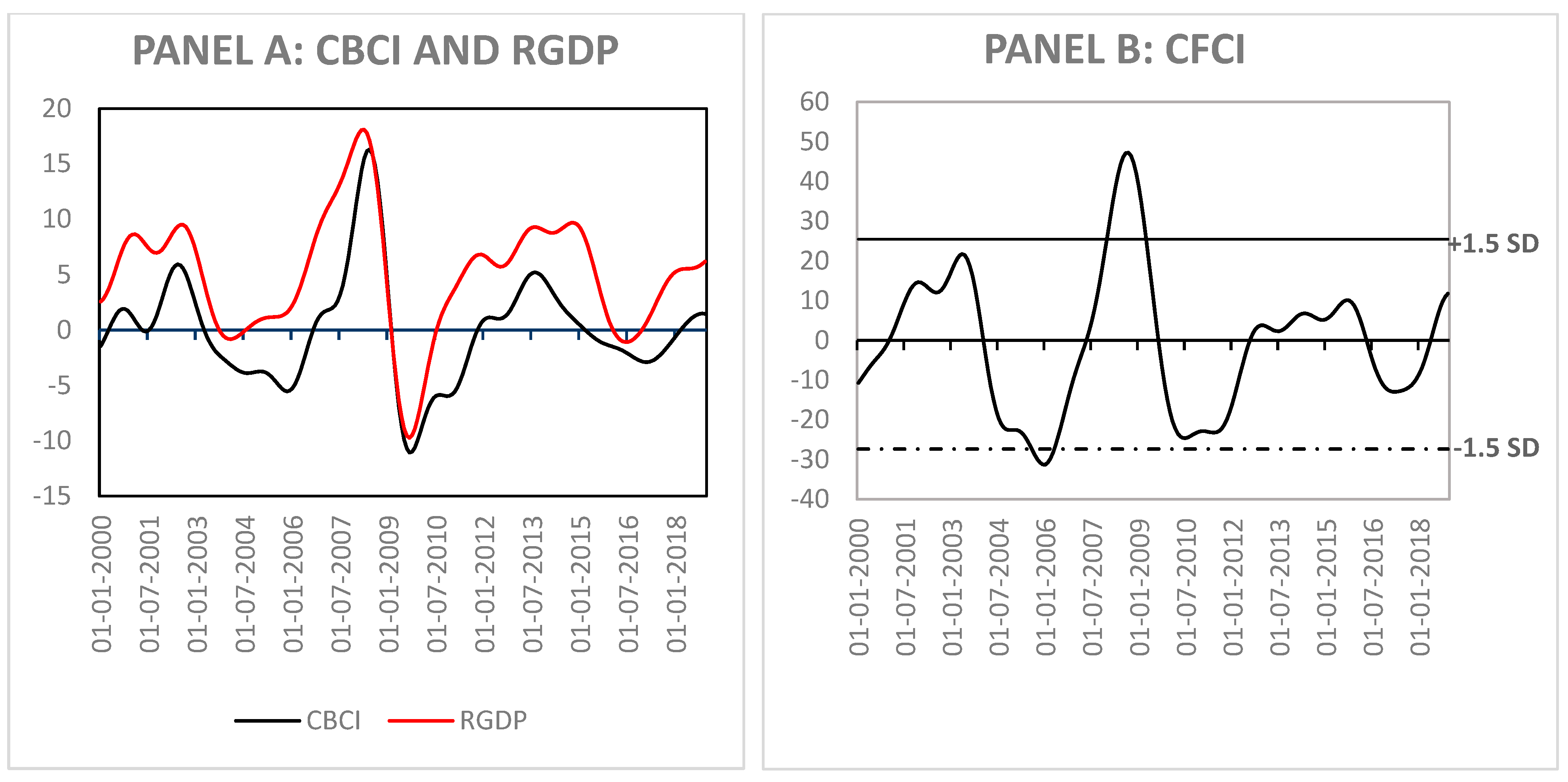
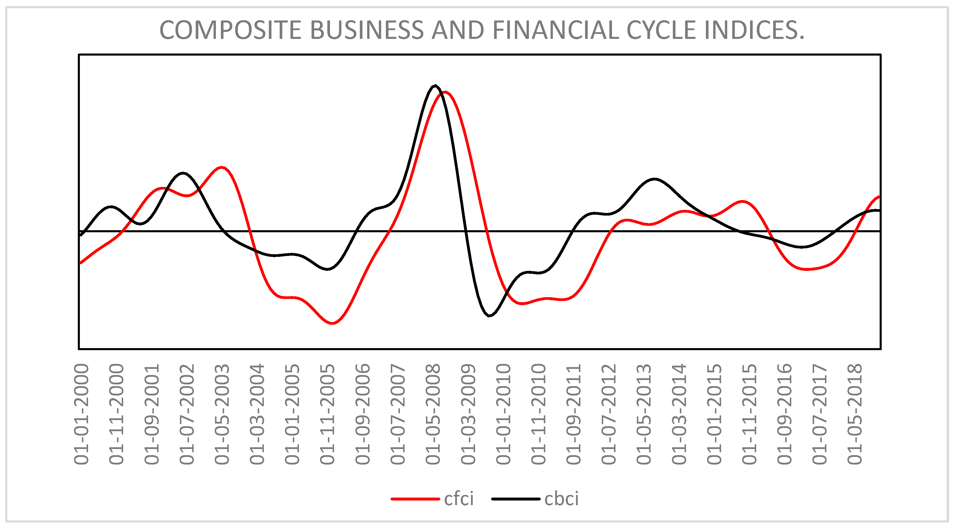
4.2.1. Graphical Illustration of the Interactions between CBCI and CFCI

This section presents results on the interactions between the MaPP and MP policies based on the interactions of BCs and FCs. Initially, this section provides a graphical illustration of these indices which is shown in Figure 2: showing CFCI as the red graph and CBCI as the black graph. The figure shows that the two indices follow the same path, with CBCI leading CFCI. While noting a few instances of divergence (in 2002/07 and in 2015/11), the two indices are almost moving together as one during the periods 2007/08 and 2008/05, which marks the period during which the GFC occurred. A measure of simple correlation between the two indices equals to 0.7147 for the whole sample. This is proof of a high correlation between the two indices; thus, it can be said that about 71.46 percent of the time, these indices are moving together.

Analysing the simple correlation between the three sub periods, viz. the pre-GFC (2000M01–2006M12), GFC (2007M01–2010M12), and post-GFC (2011M01–2018M12) periods, the following results were obtained: 0.7293, 0.7302, and 0.7268, respectively. This means that prior to the GFCs, about 72.93 percent of the time, the two indices were moving together; further, during the crisis period, about 73.02 percent of the time, the indices were moving together; and post GFCs, about 72.68 percent of the time, the indices were moving together.

This is evidence of the close association of BCs and FCs, as found in the literature. It is further proof that the two cycles tend to be highly interrelated during periods of financial distress. While graphical illustration of the interactions between indices is only a first step towards understanding their dynamics, the present section also provides statistical analysis to further broaden the reader’s understanding of the interactions between these indices.

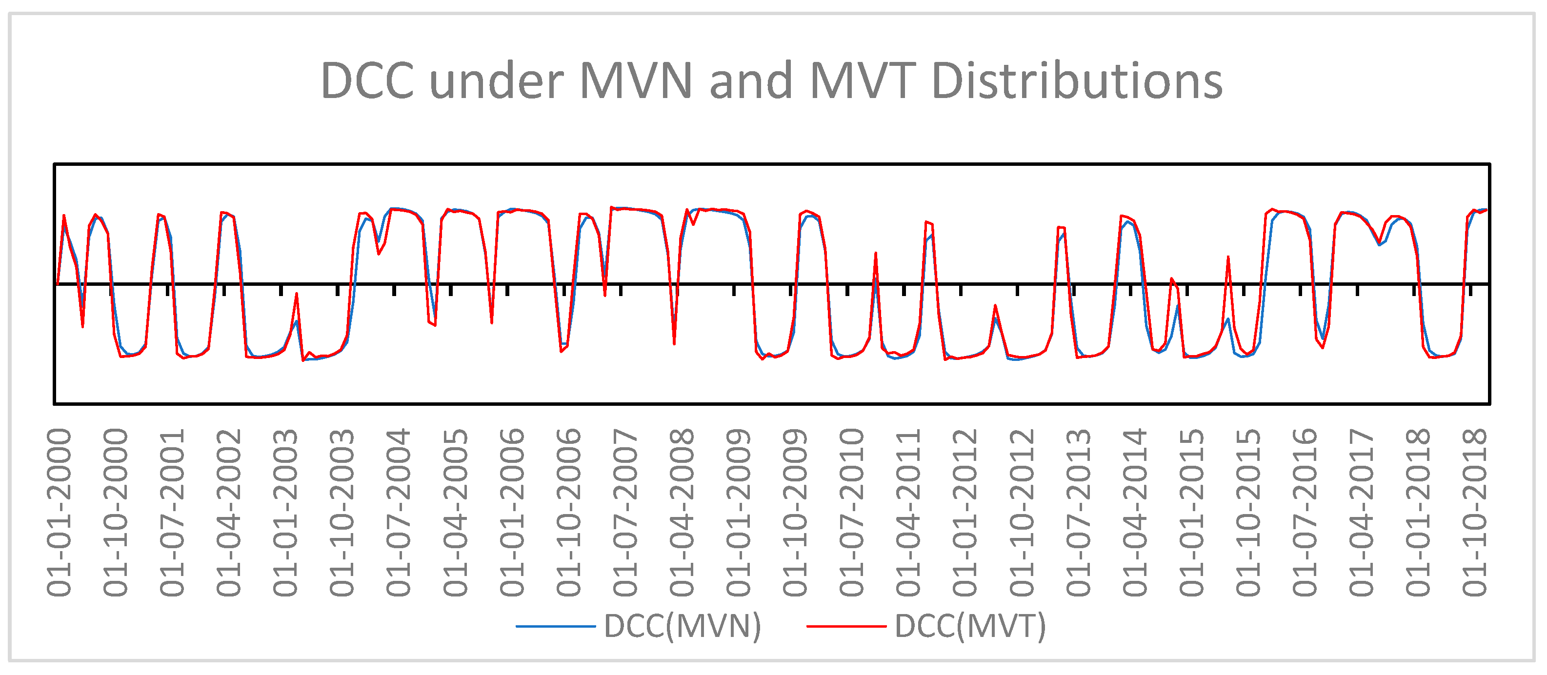
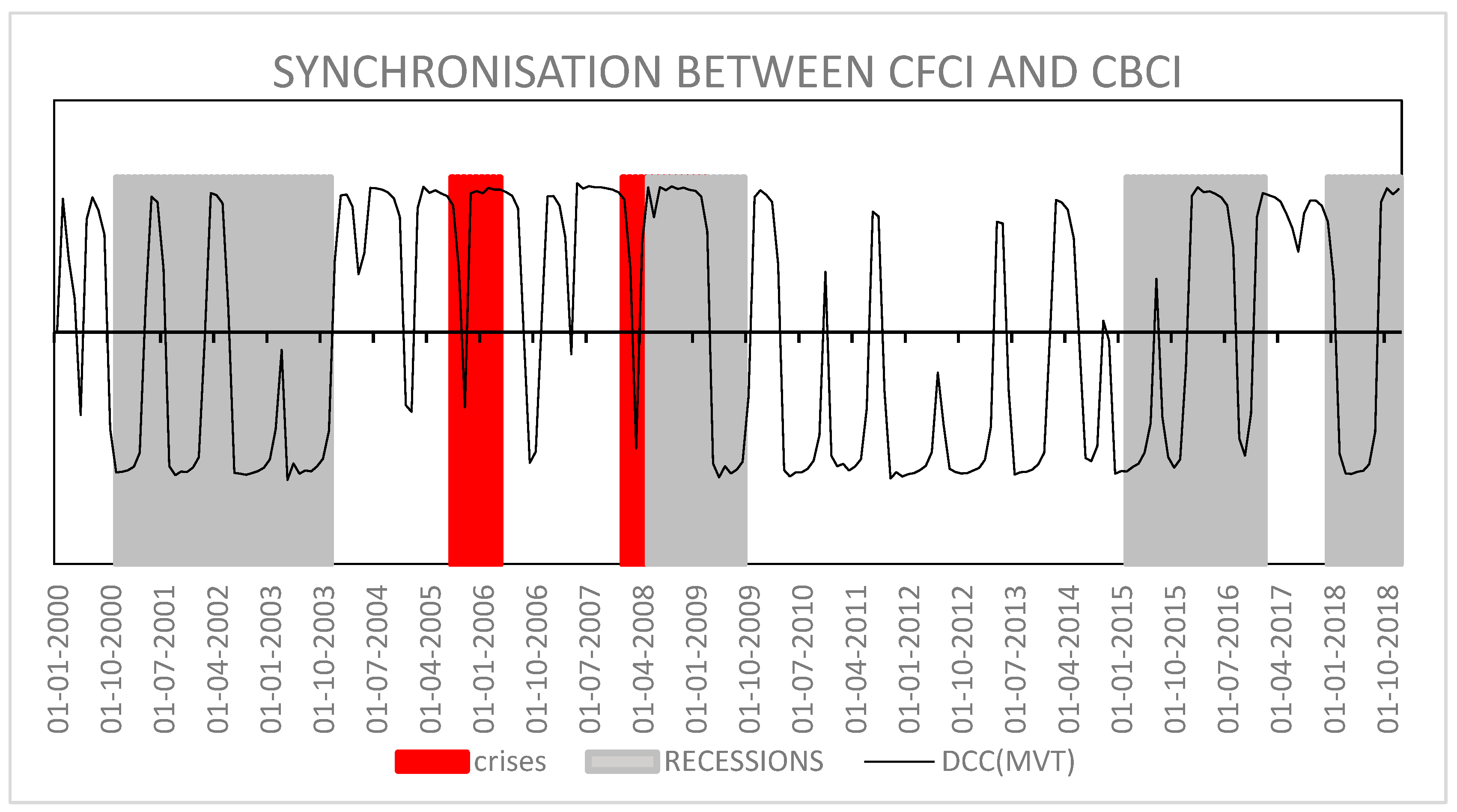
4.2.2. Synchronisation between CFCI and CBCI

The present sub-section provides synchronisation results from both the two-step DCC and ADCC MGARCH models. Through the adoption of Bayesian information criteria (BIC), a GARCH (1,1) model was selected at the initial stage, as this possessed the lowest BIC score. The research then estimated the DCC and the ADCC models under both the multivariate normal (MVN) and the multivariate student $t$ (MVT) distributions. This was performed for comparison purposes, as the MVN test initially indicated that the data were not multivariate normally distributed. The parameter estimates of these models are shown in

Table 3. Parameter estimates of the DCC and the ADCC.

	DCC (MVN)	ADCC (MVN)	DCC (MVT)	ADCC (MVT)
$a$	0.731 ***	0.731 ***	0.854 ***	0.855 ***
$b$	0.198 ***	0.198 **	0.060 *	0.060 *
$g$	-	0	-	0
$Shape$	-	-	50.000 ***	50.000 ***
$LL$	752.70	752.70	766.01	767.34

NB: Significance levels: *** 1%, ** 5%,* 10%. Source: Authors’ own estimates.

, focusing only on the joint conditional correlations and the asymmetric components.

According to Table 3, $a$ represents the dcca1 parameter, $b$ represents the dccb1 parameter, and $g$ represents the asymmetric component of the ADCC model. The $a$ and $b$ coefficients indicate whether the DCC and the ADCC models are valid for the system of series being diagnosed, while the $g$ coefficient reports the asymmetric effects of shock with the same sign in the ADCC model, thus specifying whether these are important or not in the model system.

In accordance with the above, the parameter estimates of $a$ and $b$ are statistically significant in both of the models under the different specification. This provides validity in the usage of a dynamic correlations model instead of a constant correlations model. These parameters also provide information about the short- and long-term dynamics of the system series. Accordingly, it can be deduced that the series exhibit both long-term and short-term dynamic correlations. Introducing the $g$ parameter shows no significant positive or negative effect on the strength of the correlation since the parameters are zero and insignificant under both of the distributions. Hence, it can be concluded that the asymmetric effect of shocks with the same signs does not appear to be important.

In line with the estimates of the two models, Figure 3 and Figure 4 below plot the conditional correlations graphs for each model under the different multivariate distributions, respectively.

Figure 3 above shows the DCC MGARCH graphs, with the red graph showing the conditional correlations under the MVT distribution and the black graph showing the conditional correlations under the MVN distribution. Also, Figure 4 below shows the ADCC MGARCH graphs, with the red graph showing the conditional correlations under the MVT distribution and the black graph showing the conditional correlations under the MVN distribution.

Notably, in both figures, the correlations between CFCI and CBCI are shown to vary with the varying dynamics in both the economic and financial sectors. Hence, static estimates of co-movement in this regard could produce misleading results. Further, the two models have produced identical conditional correlations under the two different distributions, with the MVT distribution conditional correlations showing larger swings than the MVN distribution conditional correlations. As a result, this suggests that both the ADCC and the DCC models are adequate in measuring the time-varying conditional correlations in that they display the mean reversion along a constant level, and control for high persistence in conditional volatility for both the system series.

Therefore, this also suggests that either of the two results can be used in this research for further analysis. Hence, taken from the above results and the results of the multivariate normality test, the following analysis relies on the results of the DCC(MVT) conditional correlations. The MVT distribution is selected here due to the fact that the MVN test showed the data are not multivariate normally distributed.

4.2.3. Interactions between MaPP and MP and Their Coordination

This sub-section uses the conditional correlations obtained in the previous sub-section to study the interactions between MaPP and MP and their possibility of coordination. Accordingly, Figure 5 shows the conditional correlations, together with the recession periods for South Africa as obtained from the OECD database, and the periods of financial crises as determined by the CFCI. For ease of interpretation of these results, the period under examination is broken down into three sub periods, namely: the pre-GFC period (2000M01–2006M12), the GFC period (2007M01–2010M12), and the post-GFC period (2011M01–2018M12). The article also compares the co-movement at times when the financial system is under stress, the real economy is in a recession, and when both the financial system and the real economy are facing no stress.

In the pre-GFC sub-period, Figure 5 shows evidence of volatile conditional correlation between CFCI and CBCI, ranging between -0.9 and 0.8, until 2003. Only after September 2003 does the correlation start taking shape and following an upwards trend, reaching a highest correlation value of 0.93 in July 2004. After that, the correlation declines but remains mostly positive during the period leading up to the beginning of the subprime mortgage crisis in the USA. This instability in correlation between CFCI and CBCI in this sub-period may be a result of the dotcom bubble burst, which took place between March 2000 and December 2001.

Interestingly, in the GFC sub-period, there is no clearly consistent increase or decrease in the co-movement between the CFCI and CBCI. However, it is worth noting also that the co-movement remains mostly positive and strong during this period. Only from February 2009 is a dramatic decline observed in the co-movement between the two cycles leading up to May 2010. Then, afterwards, high volatility is observed in the co-movement leading up to the end of the GFC sub-period in December 2010. In line with Gökalp and Yu (2018), Figure 5 also shows that in the immediate aftermath of the GFC, the co-movement between the two cycles declined. Therefore, the relationship between the cycles broke after the GFC and remained mostly negative throughout most of the post-GFC sub-period.

These results suggest that when the real economy is faced with considerable stress and the economy is in a recession, there is higher volatility in the co-movement between the business and financial cycles in South Africa. However, when the financial system is under so much stress that there are financial crises in the country, the two cycles tend to highly co-move with fewer instances of divergence. Under normal times, where neither the financial system nor the real economy is under considerable stress, the two cycles tend to move in opposite directions, which is shown by the negative co-movement in the post GFC sub-period.

Part of the contribution of this article is to link the synchronization analysis of CBCI and CFCI to the interactions between MaPP and MP and their coordination, respectively. With Dunstan (2014), Frait et al. (2014), and Spencer (2014), the researchers are of the view that the coordination between MaPP and MP is based on BCs and FCs synchronization. The article further adopted the Metcalfe (1994) scale of coordination to study the levels of coordination that may be achieved between these two policies. While this was originally developed to study coordination between ministries, this article utilises the ideas behind its use, with a few modifications and additions which are in line with the analysis of coordination between MaPP and MP, on the basis of BCs and FCs synchronization.

In view of the above, the article assigned degrees of synchronization to CBCI and CFCI on the corresponding levels of coordination between MaPP and MP. It remains imperative to note that this combination of ideas is purely an author’s thinking on how intersections between BCs and FCs can be useful for purposes of coordination between MaPP and MP.

Table 4. The Modified Version of the Metcalfe (1994) Scale of Coordination.

Level 8: Establishing central priorities desynchronization between BCs and FCs

Level 7: Setting limits on policy actions desynchronization between BCs and FCs

Level 6: Arbitration of policy differences desynchronization between BCs and FCs

Level 5: Search for agreement among MaPP and MP desynchronization between BCs and FCs

Level 4: Avoid divergences among MaPP and MP 0%―39% synchronization between BCs and FCs

Level 3: Consultation and feedback between MaPP and MP 40%―59% synchronization between BCs and FCs

Level 2: Communication between each other (MaPP and MP) 60%―79% synchronization between BCs and FCs

Level 1: Independent decision-making by MaPP and MP 80%―100% synchronization between BCs and FCs

Source: adopted from Metcalfe (1994) and modified by author.

illustrates the modified version of the Metcalfe (1994) scale of coordination.

The information in Table 4 is what is referred to here as the degrees of coordination between MaPP and MP based on BCs and FCs synchronization, shown in line with Figure 5 above. At the lowest level of the table (Level 1), there exists the greatest degree of synchronization (80–100%) between CBCI and CFCI, so much so that the two cycles are moving together as one line. These are situations in which a tightening of MP in response to strong growth in inflationary pressures is associated with a tightening of MaPP in response to booming asset prices and credit growth. Assuming each policy is able to achieve its objective, there will be no need for policy coordination; therefore, policy decisions are complementary.

The analysis of Figure 5 above shows the persistent prevalence of this level of coordination in the period under examination. It shows this to be mostly common under situations when both the financial system and the real economy are under considerable stress. For example, synchronisation is volatile and reaches values as high as 92% between the period July 2001 and March 2006, a period with both a recession and a financial calamity. The cycles become even more synchronised during the 2007–2009 GFC period, reaching the highest level, of 94%, in September 2008, a period which has seen a simultaneous occurrence of financial crises and recessions. Fewer instances of this level of coordination are seen in the post-GFC period, such as in the period October 2018, where synchronisation is volatile and reaches values as high as 93%.

When CBCI and CFCI are 60–79% synchronized, policymakers are at Level 2 of coordination between MaPP and MP, according to Table 4 above. At this level, the two policy agents start to acknowledge the potential interactions between the two policy decisions; hence, they serve to ensure that each agent is informed about the others’ actions. Again, a greater degree of complementarity in the policy decisions exists, which leads to a limited or no need for coordination. The analysis in Figure 5 shows very few instances of this kind of coordination, an example of which is seen in the period of August 2011 and May 2013. In this period, synchronisation becomes as high as 74%, thus pointing to a limited or no need for coordination at that point in time.

A scant degree of synchronization (40–59%) between these cycles calls for a two-way communication during policy planning through consultation and feedback (Level 3). This is a stage of understanding the nature of the interactions between the two policies and the realization of the need to coordinate policy decisions in practice. At 0–39% degrees of synchronization, the agents realize the potential divergences and losses that may arise due to a lack of coordination between the two policies; therefore, they act to avoid these divergences (Level 4). Thus, this calls for a great degree of coordination between MaPP and MP. The analysis in Figure 5 shows no clear evidence of this kind of coordination in the period under examination, except in the period July 2015, where synchronisation becomes 34%, hence requiring the avoidance of divergences that may arise in policy decision making, henceforth calling for a great degree of coordination.

When BCs and FCs are out of sync, meaning desynchronized, as shown in Levels 5 to 8 of Table 4 and the post-GFC period between July 2009 and October 2015, the policy decisions of MaPP and MP are noncomplementary; therefore, there exists a greater potential for conflict. As a result, the primary objectives of the two policies will need to be carefully balanced, thus calling for the greatest degree of coordination between the two policy decisions. A lack of coordination in such situations involves the risk of welfare loss, as each policy seeks to overly counteract the impact of the other’s objective on its own.

4.2.4. Discussion of Findings

The first set of results indicates that there exists a financial cycle in South Africa, which coincides closely with the business cycle, with its length longer than that of the BC. Further, the BC seems to lead this FC, which is in line with current theoretical and empirical analyses. As is expected, monetary policy measures are implemented immediately with a short delay, while macroprudential policy measures are usually announced well in advanced and implemented with a relatively long delay. This is proof of the dynamic inconsistency that exists within each policy setting, which thus far remains difficult to capture within the existing modelling frameworks. In accordance with de Paoli and Paustian (2017), one solution is to let MaPP instruments be chosen first on the basis that macroprudential authority is often seen to move at a slower frequency.

What is clear from the second set of results is the fact that BCs and FCs are mostly synchronised rather than desynchronised in South Africa. This is especially true when the real economy is under considerable stress, and thus faced with recessions, and more especially when there are financial crises. However, under normal times when both the financial system and the real economy are not facing any pressure from stress, the two cycles are desynchronised. Therefore, it can be said that under conditions of financial and real economic stress in South Africa, when there is crisis management rather than crisis prevention, MaPP and MP decisions are complementary. As a result, coordination is relatively simple, simply requiring each policy to cater for the complementarity effects of the other. At times, there will be a limited or no need for coordination between the two policy decisions. Such findings are similar to the clear separation view of MaPP and MP interactions, also referred to as the modified Jackson Hole Consensus.

However, under normal conditions when there is crisis prevention rather than crisis management, MaPP and MP decisions are noncomplementary; therefore, there is a greater potential for conflict between the two policy decisions. In this case, the two policy objectives will need to be carefully balanced, which calls for the greatest degree of coordination between the two policy decisions. These results are consistent with those found in Billio and Petronevich (2017), who found that synchronisation of BCs and FCs will depend largely on which phase of the cycles the economy is in. Further, these are consistent with the conclusions of Constâncio et al. (2019), who revealed that the two cycles are not always synchronised; hence, policies that target the FC powerfully complement policies that target the BC. Such findings are in agreement with the second strand of the literature which considers MaPP and MP objectives as inseparable, thus advocating for the need for coordination.

5. Conclusions and Recommendations

The present article contributes to the relatively scant literature on macroeconomic policy coordination in South Africa, in the following ways: firstly, through the adoption of a two-step Markov switching dynamic factor model, the research measured both the composite business and financial cycle indices. Secondly, the question of whether BCs and FCs are synchronized in SA was investigated, and if so, whether it is possible to coordinate MaPP and MP based on this synchronicity. As a response, the article adopted the time varying DCC MGARCH model of Engle (2002) together with the ADCC MGARCH model of Cappiello et al. (2006) to empirically investigate synchronization between BCs and FCs in South Africa. Lastly, using the knowledge of the synchronicity between these cycles, the article has provided new evidence on interactions between MaPP and MP and their coordination, through the adoption of the modification Metcalfe (1994) scale of coordination.

The results showed that when both the South African financial system and real economy are under considerable stress, BCs and FCs are synchronised. Therefore, MaPP and MP decisions will be complementary. As a result, a modified Jackson Hole Consensus will hold. However, under normal times when both the financial system and real economy are facing no pressure from stress, BCs and FCs are desynchronised in South Africa. At such times, policy decisions are noncomplementary. As a result, there will be a greater potential for conflict between the two policy decisions, thus requiring that the policy objectives be carefully balanced. This calls for the greatest degree of coordination between the two policy decisions. Hence, the advocacy for coordination will hold. This therefore is proof that the South African economy moves from one strand of the literature to the next depending on which phase of BCs and FCs the economy is in.

Overall, these results are proof that it is possible to coordinate the conduct of MaPP and MP based on the synchronicity of BCs and FCs. Further, these results are proof that the economy may move from one strand to any strand of the literature as mentioned above, depending on which state of BCs and FCs the economy is in. A noteworthy observation is that the findings in this article contradict those found in Svensson (2018), which suggests that under normal times when there is crisis prevention, the two policies are better conducted separately, and in crises times when there is crisis management, the two policies are better conducted co-ordinately. These findings, therefore, add new empirical evidence in developing countries, as opposed to developed countries or a group of developed countries, about the interactions between MaPP and MP based on the interactions between BCs and FCs and their possibility of coordination, respectively.

Furthermore, while these results reveal a clear reason for coordination of MaPP and MP in South Africa in cases where BCs and FCs are moving in opposite directions, it is recommended that such coordination must be conditional on each policy arm continuing to focus on its own primary objectives. Failure to do this may lead to complicated policy decisions, undermine transparency, and potentially be damaging to the credibility of both MaPP and MP. Furthermore, the failure to coordinate the two policy decisions at times when it is required may lead to welfare losses. Finally, it is noteworthy that such findings are currently aligned with the cyclical component of systemic risk. Future studies may focus on the structural component of systemic risk in producing analysis of this kind.

References

1. Adrian, Tobias, and Nellie Liang. 2016. Monetary Policy, Financial Conditions, and Financial Stability. Available online: https://www.newyorkfed.org/medialibrary/media/research/staff_reports/sr690.pdf (accessed on 18 September 2023).
2. Adrian, Tobias, Arturo Estrella, and Hyun Song Shin. 2010. Monetary Cycles, Financial Cycles and the Business Cycle (1 January 2010). FRB of New York Staff Report No. 421. New York: FRB of New York. [Google Scholar] [CrossRef]
3. Agénor, Pierre-Richard, Koray Alper, and Luiz Pereira da Silva. 2013. Capital regulation, monetary policy and financial stability. International Journal of Central Banking 9: 193–238. [Google Scholar]
4. Agur, Itai. 2019. Monetary and macroprudential policy coordination among multiple equilibria. Journal of International Money and Finance 96: 192–209. [Google Scholar] [CrossRef]
5. Ahmed, Jameel, Sajid M. Chaudhry, and Stefan Straetmans. 2018. Business and financial cycles in the Eurozone: Synchronization or decoupling. The Manchester School 86: 358–89. [Google Scholar] [CrossRef]
6. Akar, Cüneyt. 2016. Analyzing the Synchronization between the Financial and Business Cycles in Turkey. Journal of Review on Global Economics 5: 25–35. Available online: https://ssrn.com/abstract=2913550 (accessed on 18 September 2023). [CrossRef]
7. Artis, Mike, Hans-Martin Krolzig, and Juan Toro. 2004. The European business cycle. Oxford Economic Papers 56: 1–44. [Google Scholar] [CrossRef]
8. Billio, Monica, and Anna Petronevich. 2017. Dynamical Interaction between Financial and Business Cycles (15 October 2017). University Ca’ Foscari of Venice, Department of Economics Research Paper Series No. 24/WP/2014; Venezia: University Ca’ Foscari of Venice. [Google Scholar] [CrossRef]
9. Bollerslev, Tim. 1990. Modelling the coherence in short-run nominal exchange rates: A multivariate generalized ARCH model. The Review of Economics and Statistics 72: 498–505. Available online: https://public.econ.duke.edu/~boller/Published_Papers/restat_90.pdf (accessed on 18 September 2022). [CrossRef]
10. Borio, Claudio. 2014a. Monetary Policy and Financial Stability: What Role in Prevention and Recovery? Available online: https://www.bis.org/publ/work440.htm (accessed on 18 September 2022).
11. Borio, Claudio. 2014b. The financial cycle and macroeconomics: What have we learnt? Journal of Banking & Finance 45: 182–98. [Google Scholar]
12. Borio, Claudio, Craig Furfine, and Philip Lowe. 2001. Procyclicality of the financial system and financial stability: Issues and policy options. BIS Papers 1: 1–57. [Google Scholar]
13. Bosch, Adél, and Franz Ruch. 2013. An Alternative Business Cycle Dating Procedure for South Africa. South African Journal of Economics 81: 491–516. [Google Scholar] [CrossRef]
14. Bosch, Adél, and Steven F. Koch. 2020. The South African financial cycle and its relation to household deleveraging. South African Journal of Economics 88: 145–73. [Google Scholar] [CrossRef]
15. Cagliarini, Adam, and Fiona Price. 2017. Exploring the Link between the Macroeconomic and Financial Cycles. In Monetary Policy and Financial Stability in a World of Low Interest Rates; Edited by Jonathan Hambur and John Simon. Reserve Bank of Australia. Available online: https://www.rba.gov.au/publications/confs/2017/pdf/rba-conference-volume-2017-cagliarini-price.pdf (accessed on 18 September 2023).
16. Cappiello, Lorenzo, Robert F. Engle, and Kevin Sheppard. 2006. Asymmetric dynamics in the correlations of global equity and bond returns. Journal of Financial Econometrics 4: 537–72. [Google Scholar] [CrossRef]
17. Chorafas, Dimitris N. 2015. Financial cycles. In Financial Cycles: Sovereigns, Bankers, and Stress Tests. New York: Palgrave Macmillan US, pp. 1–24. Available online: https://link.springer.com/chapter/10.1057/9781137497987_1 (accessed on 18 September 2022).
18. Choudhry, Taufiq, Fotios I. Papadimitriou, and Sarosh Shabi. 2016. Stock market volatility and business cycle: Evidence from linear and nonlinear causality tests. Journal of Banking & Finance 66: 89–101. [Google Scholar]
19. Claessens, Stijn. 2013. Interactions between Monetary and Macroprudential Policies in an Interconnected World. Paper presented at Bank of Thailand-IMF Conference on Monetary Policy in an Interconnected World, Bangkok, Thailand, November 1–2; vol. 31. Available online: https://www.bcu.gub.uy/Comunicaciones/DCI_Interno/Claessens%20-%20Interactions%20between%20Monetary%20and%20Macroprudential%20Policies%20in%20an%20Interconnected%20World.pdf (accessed on 18 September 2022).
20. Claessens, Stijn, M. Ayhan Kose, and Marco E. Terrones. 2011. Financial cycles: What? how? when? In NBER International Seminar on Macroeconomics. Chicago: University of Chicago Press, vol. 7, pp. 303–44. [Google Scholar]
21. Claessens, Stijn, M. Ayhan Kose, and Marco E. Terrones. 2012. How do business and financial cycles interact? Journal of International Economics 87: 178–90. [Google Scholar] [CrossRef]
22. Comrey, Andrew L., and Howard B. Lee. 2013. A First Course in Factor Analysis. New York: Psychology Press. [Google Scholar] [CrossRef]
23. Constâncio, Vítor, Inês Cabral, Carsten Detken, John Fell, Jérôme Henry, Paul Hiebert, Sujit Kapadia, Sergio Nicoletti Altimar, Fatima Pires, and Carmelo Salleo. 2019. Macroprudential Policy at the ECB: Institutional Framework, Strategy, Analytical Tools and Policies. Strategy, Analytical Tools and Policies (July). Available online: https://www.ecb.europa.eu/pub/pdf/scpops/ecb.op227~971b0a4996.en.pdf (accessed on 18 September 2022).
24. de Paoli, Bianca, and Matthias Paustian. 2017. Coordinating monetary and macroprudential policies. Journal of Money, Credit and Banking 49: 319–49. [Google Scholar] [CrossRef]
25. Doz, Catherine, and Anna Petronevich. 2016. Dating business cycle turning points for the french economy: An MS-DFM approach. In Dynamic Factor Models. Bingley: Emerald Group Publishing Limited, pp. 481–538. [Google Scholar] [CrossRef]
26. Drehmann, Mathias, Claudio Borio, and Konstantinos Tsatsaronis. 2012. Characterising the Financial Cycle: Don’t Lose Sight of the Medium Term! (June 1). BIS Working Paper No. 380. Available online: https://ssrn.com/abstract=2084835 (accessed on 18 September 2022).
27. Dunstan, Ashley. 2014. The interaction between monetary and macro-prudential policy. Reserve Bank of New Zealand Bulletin 77: 15–25. [Google Scholar]
28. Engle, Robert. 2002. Dynamic conditional correlation: A simple class of multivariate generalized autoregressive conditional heteroskedasticity models. Journal of Business & Economic Statistics 20: 339–50. [Google Scholar]
29. Farrell, Greg, and Esti Kemp. 2020. Measuring the financial cycle in South Africa. South African Journal of Economics 88: 123–44. [Google Scholar] [CrossRef]
30. Frait, Jan, and Zlatuše Komárková. 2010. Financial stability, systemic risk and macroprudential policy. Financial Stability Report 2011: 96–111. [Google Scholar]
31. Frait, Jan, Simona Malovaná, and Vladimír Tomšík. 2014. The interaction of monetary and macroprudential policies in the pursuit of the central bank’s primary objectives. CNB Financial Stability Report 2015: 110–20. [Google Scholar]
32. Gächter, Martin, Aleksandra Riedl, and Doris Ritzberger-Grünwald. 2012. Business cycle synchronization in the euro area and the impact of the financial crisis. Monetary Policy & the Economy 2: 33–60. [Google Scholar]
33. Ghalanos, Alexios. 2019. The RMGARCH Models: Background and Properties. Version 1.3-0. Available online: https://mran.microsoft.com (accessed on 19 June 2021).
34. Gogas, Periklis, and George Kothroulas. 2009. Two Speed Europe and Business Cycle Synchronization in the European Union: The Effect of the Common Currency. MPRA Paper. Available online: https://mpra.ub.uni-muenchen.de/id/eprint/13909 (accessed on 18 September 2022).
35. Gökalp, Bekir Tamer, and Xingkai Yu. 2018. Do the Business Cycles and Financial Cycles Move Together in Turkey? Journal of Advances in Economics and Finance 3: 19–26. [Google Scholar] [CrossRef]
36. Hamilton, James D. 1989. A new approach to the economic analysis of nonstationary time series and the business cycle. Econometrica: Journal of the Econometric Society 57: 357–84. [Google Scholar] [CrossRef]
37. Hodula, Martin, Jan Janků, and Lukáš Pfeifer. 2023. Macro-prudential policies to contain the effect of structural risks on financial downturns. Journal of Policy Modeling. [Google Scholar] [CrossRef]
38. Hollander, Hylton, and Dawie Van Lill. 2019. A Review of the South African Reserve Bank’s Financial Stability Policies. Working Papers 11/2019, Stellenbosch University, Department of Economics. Available online: https://ideas.repec.org/p/sza/wpaper/wpapers325.html (accessed on 18 September 2022).
39. Jeantheau, Thierry. 1998. Strong consistency of estimators for multivariate ARCH models. Econometric Theory 14: 70–86. [Google Scholar] [CrossRef]
40. Kim, Chang-Jin. 1994. Dynamic linear models with Markov-switching. Journal of Econometrics 60: 1–22. [Google Scholar] [CrossRef]
41. Kim, Myung-Jig, and Ji-Sung Yoo. 1995. New index of coincident indicators: A multivariate Markov switching factor model approach. Journal of Monetary Economics 36: 607–30. [Google Scholar] [CrossRef]
42. Kokores, Ioanna. 2015. Lean-against-the-wind monetary policy: The post-crisis shift in the literature. SPOUDAI Journal of Economics and Business 65: 66–99. [Google Scholar]
43. Kose, M. Ayhan, Christopher Otrok, and Eswar Prasad. 2012. Global Business Cycles: Convergence or Decoupling? International Economic Review 53: 511–38. Available online: http://www.jstor.org/stable/23251597 (accessed on 18 September 2023). [CrossRef]
44. Krznar, Ivo. 2011. Identifying Recession and Expansion Periods in Croatia. CNB Istraživanja. Available online: https://www.hnb.hr/repec/hnb/wpaper/pdf/w-029.pdf (accessed on 18 September 2023).
45. Krznar, Ivo, and Troy D. Matheson. 2017. Financial and Business Cycles in Brazil. International Monetary Fund. Available online: https://www.imf.org/en/Publications/WP/Issues/2017/01/24/Financial-and-Business-Cycles-in-Brazil-44577 (accessed on 18 September 2023).
46. Leamer, Edward E. 2007. Housing is the Business Cycle. No. w13428. Kansas City: Federal Reserve Bank of Kansas City, pp. 149–233. [Google Scholar]
47. Liu, Guangling, and Thabang Molise. 2020. The optimal monetary and macroprudential policies for the South African economy. South African Journal of Economics 88: 368–404. [Google Scholar] [CrossRef]
48. Ma, Yong, and Jinglan Zhang. 2016. Financial cycle, business cycle and monetary policy: Evidence from four major economies. International Journal of Finance & Economics 21: 502–27. [Google Scholar]
49. Malovana, Simona, and Jan Frait. 2017. Monetary policy and macroprudential policy: Rivals or teammates? Journal of Financial Stability 32: 1–16. [Google Scholar] [CrossRef]
50. Malovaná, Simona, Martin Hodula, Zuzana Gric, and Josef Bajzík. 2023. Macroprudential policy in central banks: Integrated or separate? Survey among academics and central bankers. Journal of Financial Stability 65: 101107. [Google Scholar] [CrossRef]
51. Metcalfe, Les. 1994. International policy co-ordination and public management reform. International Review of Administrative Sciences 60: 271–90. [Google Scholar] [CrossRef]
52. Mink, Mark, Jan P. A. M. Jacobs, and Jakob de Haan. 2007. Measuring Synchronicity and Co-Movement of Business Cycles with an Application to the Euro Area. CESifo Working Paper, No. 2112. Munich: Center for Economic Studies and ifo Institute (CESifo). Available online: http://hdl.handle.net/10419/26157 (accessed on 18 September 2023).
53. Nzimande, Ntokozo Patrick, and Harold Ngalawa. 2016. Is There a SADC Business Cycle? Evidence from a Dynamic Factor Model. Economic Research Southern Africa. Available online: https://policycommons.net/artifacts/2120725/is-there-a-sadc-business-cycle-evidence-from-a-dynamic-factor-model/2876023/ (accessed on 20 September 2022).
54. Oman, William. 2019. The synchronization of business cycles and financial cycles in the euro area. International Journal of Central Banking 15: 327–62. [Google Scholar]
55. Pan, Haifeng, and Dingsheng Zhang. 2020. Coordination Effects and Optimal Policy Choices of Macroprudential Policy and Monetary Policy. Complexity 2020: 1–11. [Google Scholar] [CrossRef]
56. Pineda, Emilio, Paul Anthony Cashin, and Yan Sun. 2009. Assessing Exchange Rate Competitiveness in the Eastern Caribbean Currency Union. Available online: https://www.imf.org/external/pubs/ft/wp/2009/wp0978.pdf (accessed on 18 September 2023).
57. Rünstler, Gerhard, and Marente Vlekke. 2015. Business and Financial Cycles: An Unobserved Components Models Perspective. European Central Bank. Available online: https://scholar.google.com/scholar?hl=en&as_sdt=0%2C5&q=R%C3%BCnstler%2C+Gerhard%2C+and+Marente+Vlekke.+%22Business+and+financial+cycles%3A+an+unobserved+components+models+perspective.%22+European+Central+Bank+%282015%29.+&btnG= (accessed on 18 September 2023).
58. Sala-Rios, Mercè, Teresa Torres-Solé, and Mariona Farré-Perdiguer. 2016. Credit and business cycles’ relationship: Evidence from Spain. Portuguese Economic Journal 15: 149–71. [Google Scholar] [CrossRef]
59. Savva, Christos S., Kyriakos C. Neanidis, and Denise R. Osborn. 2010. Business cycle synchronization of the euro area with the new and negotiating member countries. International Journal of Finance & Economics 15: 288–306. [Google Scholar]
60. Seo, Joo Hwan, Sung Yong Park, and Larry Yu. 2009. The analysis of the relationships of Korean outbound tourism demand: Jeju Island and three international destinations. Tourism Management 30: 530–43. [Google Scholar] [CrossRef]
61. Smets, Frank. 2018. Financial stability and monetary policy: How closely interlinked? International Journal of Central Banking 10: 263–300. [Google Scholar]
62. South African Reserve Bank. 2016. A New Macroprudential Policy Framework for South Africa. Pretoria: Financial Stability Department. Available online: https://www.resbank.co.za/content/dam/sarb/what-we-do/financial-stability/A%20new%20macroprudential%20policy%20framework%20for%20South%20Africa.pdf (accessed on 18 September 2023).
63. Spencer, Grant. 2014. Coordination of Monetary Policy and Macro-Prudential Policy. In Speech Delivered to Credit Suisse Asian Investment Conference in Hong Kong. Available online: https://www.rbnz.govt.nz/hub/publications/speech/2014/speech2014-03-27 (accessed on 18 September 2023).
64. Stock, James H., and Mark W. Watson. 2003. Forecasting output and inflation: The role of asset prices. Journal of economic literature 41: 788–829. [Google Scholar] [CrossRef]
65. Svensson, Lars E. O. 2018. Monetary policy and macroprudential policy: Different and separate? Canadian Journal of Economics/Revue Canadienne D’économique 51: 802–27. [Google Scholar] [CrossRef]
66. Tse, Yiu Kuen, and Albert K. C. Tsui. 2002. A multivariate generalized autoregressive conditional heteroscedasticity model with time-varying correlations. Journal of Business & Economic Statistics 20: 351–62. [Google Scholar]
67. Tsiakas, Ilias, and Haibin Zhang. 2023. On the direction of causality between business and financial cycles. Journal of Risk and Financial Management 16: 430. [Google Scholar] [CrossRef]
68. Venter, Johann Christoffel. 2009. Business Cycles in South Africa during the Period 1999 to 2007. Pretoria: South African Reserve Bank. Available online: https://www.resbank.co.za/content/dam/sarb/publications/quarterly-bulletins/quarterly-bulletin-publications/2009/4051/Article---Business-cycles-in-South-Africa-during-the-period-1999-to-2007.pdf (accessed on 18 September 2023).
69. Vermeulen, Cobus, A. Bosch, J. Rossouw, and F. Joubert. 2017. From the business cycle to the output cycle: Predicting South African economic activity. Studies in Economics and Econometrics 41: 111–33. [Google Scholar] [CrossRef]
Figure 1. DFM-SSF AND PCA Composite Business and Financial Cycle Indices. Source: Authors’ own estimates.
Economies 11 00272 g001
Figure 2. Interactions between CBCIs and CFCIs. Source: Authors’ own estimates.
Economies 11 00272 g002
Figure 3. DCC-MGARCH graphs. Source: Authors’ own estimates.
Economies 11 00272 g003
Figure 4. ADCC-MGARCH graphs. Source: Authors’ own estimates.
Economies 11 00272 g004
Figure 5. Synchronisation between CFCI and CBCI. Source: Authors’ own estimates.
Economies 11 00272 g005