Unraveling Ghana’s Resource Curse Hypothesis: Analyzing Natural Resources and Economic Growth with a Focus on Oil Exploration

Abstract

This study examines the intricate relationship between natural resource abundance, with a specific focus on oil production, and its impact on economic growth in Ghana. Through the application of the robust Fully Modified OLS methodology and using data spanned from 1960–2021 the research underscores the essential inclusion of oil as a significant variable in comprehending economic growth dynamics. Contrary to traditional resource curse theories, the study unveils a positive nexus between oil production and economic growth, particularly within a comprehensive variable framework. This finding challenges simplistic resource curse notions and underscores the need for a holistic economic perspective. Overall, the results show that the impact of oil production on economic growth is sensitive to the inclusion or exclusion of other variables in the model. In Model 1, where all variables are included, oil production has a significant positive (0.0112**) impact on growth. Ghana’s success in avoiding the resource curse is attributed to a multifaceted strategy encompassing diversified economic approaches, transparent governance, and responsible oil revenue management. Importantly, the inclusion of oil as a pivotal variable is well-justified by its tangible contributions to economic growth. The observed positive impacts emphasize the benefits of harnessing oil resources while maintaining a holistic view of the broader economic context. Looking ahead, the insights inform policymakers in resource-rich nations, illustrating how strategic resource management—illustrated by oil—can drive resilient and comprehensive economic growth. Ghana’s experience serves as a compelling template for informed policy decisions, offering valuable lessons for achieving sustainable prosperity.

1. Introduction

The world is richly endowed with an array of natural resources, encompassing valuable mineral deposits such as gold, oil, diamonds, arable land, and more (Dorm-Adzobu 1982) The prevailing belief suggests that regions blessed with abundant resources should experience accelerated growth and development compared to those with scarce endowments. However, this relationship is not universally applicable, as evidenced by the striking disparity between Europe and Sub-Saharan Africa. While Sub-Saharan Africa boasts larger natural resource deposits, the average per capita income in the region stands at $1645, significantly lower than Europe’s $38,234 (World Bank 2022). This enigmatic phenomenon is known as the resource curse hypothesis, which has been extensively tested across diverse countries, periods, variables, and methodologies, yielding varying results.

Even in the context of Ghana, where the resource curse hypothesis has been subject to scrutiny, several issues remain unresolved and warrant further investigation. Ghana’s economy presents an intriguing scenario, characterized by abundant natural resources, including gold, oil, diamonds, manganese, limestone, bauxite, iron ore, and forestry (Ministry of Land and Natural Resources 2021). Surprisingly, there appears to be a weak relationship between natural resources, as measured by total natural resource rent using World Development Indicators (WDI), and GDP growth, with a correlation coefficient of 0.2775 (Author’s calculation using World Bank 2022 data).

Figure 1 illustrates the dynamic relationship between GDP Growth and Natural Resource Contribution in Ghana over time. The solid line represents total natural rent, while the thin line depicts GDP growth. Notably, during the period from 1970 to 1983, when natural resource contribution was increasing, GDP growth experienced negative trends for the most part. Conversely, between 1985 and 2004, as natural resources contribution increased (except for 1998), GDP growth exhibited greater stability. Interestingly, a strong correlation (r = 0.676) between GDP growth and natural resource contribution only emerged after 2010.

One crucial aspect that has been neglected in previous works is the pivotal role of oil resources. The discovery of oil in commercial quantities has a profound influence on a country’s growth trajectory. By overlooking oil as a variable, earlier studies may have missed crucial dynamics related to the resource curse phenomenon in Ghana’s economic development (see Adu 2012; Adabor 2023). The exclusion of oil from the analysis may lead to an inaccurate depiction of the true contribution of natural resources to economic growth, potentially underestimating their overall impact on the economy.

Additionally, Ghana’s economic landscape has been significantly affected by global events, such as the COVID-19 pandemic and the World Economic crises arising from the Russian–Ukraine war, which have had ramifications on economies worldwide, including Ghana. These external shocks further complicate the understanding of the resource curse phenomenon in the context of Ghana’s unique economic conditions.

This study therefore aims to investigate the relationship between natural resources and economic growth in Ghana using data from 1960 to 2021, with a particular focus on the impact of oil exploration from 2009. The research question to be answered is does the exploration of oil affect the resource curse hypothesis position in the case of Ghana? This study used the Fully Modified Ordinary Least Square Method because of its robustness over its class of estimation techniques. This method addresses the potential presence of endogeneity, serial correlation, and heteroscedasticity in regression analysis. It is particularly valuable when studying the relationship between natural resources, economic growth, and related phenomena, where these issues are commonly encountered (Kamal et al. 2021). The rationale for using Fully Modified Ordinary Least Squared lies in its robustness and ability to provide consistent and efficient estimates, even when the data suffers from certain econometric problems (Kheifets and Phillips 2019).

The reasons for including oil as an important variable which other researchers have ignored are as follows; Missed Resource Curse Dynamics: The resource curse hypothesis suggests that countries rich in natural resources, particularly oil, may experience negative economic consequences, such as slow economic growth, increased corruption, and volatility. By neglecting oil as a variable, the study might overlook the potential presence or absence of resource curse effects in Ghana’s economic development; Inaccurate Picture of Resource Contribution: Oil is a substantial contributor to Ghana’s natural resource base. Its omission can lead to an underestimation of the overall impact of natural resources on economic growth (Srivastava and Agata Ewa 2020). Consequently, the analysis may not accurately capture the full extent of resource contributions to the economy; Misrepresentation of Growth Patterns: Ghana’s economy experienced significant changes after the discovery of oil in commercial quantities in 2007 and its subsequent production from 2010 (ISSER 2010). If the analysis excludes oil as a variable, it may fail to reflect the different growth patterns and economic behavior associated with oil exploitation, leading to misleading conclusions; Potential Spillover Effects: The oil industry can have significant spillover effects on other sectors of the economy, such as job creation, infrastructure development, and fiscal policies. Neglecting oil as a variable could underestimate or overlook these inter-sectoral linkages, providing an incomplete understanding of the economic impacts and Policy Implications: Ghana’s policymakers need accurate and comprehensive information to make informed decisions about the management of natural resources, particularly oil. If oil’s impact on economic growth is not considered, it could lead to inadequate policy recommendations and ineffective resource management strategies. The inclusion of oil as an important variable in the case of Ghana is the major difference between this study and other studies.

This study has a number of contributions to existing knowledge. Firstly, by including the oil variable in the analysis, this research provides a more comprehensive and accurate assessment of the resource curse hypothesis in Ghana. It allows for a deeper understanding of how natural resources, particularly oil, affect economic growth patterns and whether Ghana has experienced any adverse effects related to the resource curse phenomenon. Secondly, the study provides valuable insights into how the discovery of oil reserves can influence economic growth dynamics. This information is critical for policymakers, as oil discoveries can have significant implications for the country’s economic development and sustainability. Thirdly, some previous studies on Ghana’s resource curse have yielded contradictory results. By including the oil variable and extending the period to 2021, this research attempts to address potential gaps and inconsistencies in earlier findings, contributing to a more robust and cohesive body of knowledge (Miles 2017). Again, understanding the relationship between natural resources, particularly oil, and economic growth in Ghana can have significant policy implications. The findings from this study can assist policymakers in formulating effective strategies for sustainable resource management, economic diversification, and mitigating any potential adverse effects of resource dependence. Furthermore, the inclusion of the oil variable and the extension of the study period add to the existing literature on the resource curse hypothesis and its application to Ghana. This research contributes to the knowledge base by presenting updated and relevant findings that consider the country’s specific economic conditions and developments over time. Moreover, with a focus on data up to 2021 (Schweinsberg et al. 2021), this study can aid in long-term economic planning and decision-making. Policymakers and stakeholders can use the insights to anticipate future trends, assess the sustainability of resource-based growth, and develop appropriate policies to steer the economy towards resilience and stability. Lastly, while the research centers on Ghana, the findings may have implications for other resource-rich economies facing similar challenges and opportunities. The lessons learned from Ghana can inform policymakers and researchers in other countries with substantial natural resource endowments.

The rest of the study is divided into four sections. Section 2 and Section 3 address the literature review and methodology respectively. Section 4, Section 5 and Section 6 also detail the analysis of results and conclusions, and policy recommendation.

2. Literature Review

2.1. Natural Resources, Economic Growth, and Resource Curse Hypothesis

Even though it is expected natural resource abundance should help a country to develop much faster, studies have shown that natural-resource abundant economies tend to grow at a slower rate than expected (Gylfason 2000; Leite and Weidmann 1999; Sachs and Warner 1999). Over the past, countries endowed with natural resources such as Nigeria, Benin, and Venezuela have grown slowly as compared to countries such as Japan, Hong Kong, and Singapore (Papyrakis and Gerlagh 2004). This phenomenon has not been entirely true for all resources rich countries. Some countries have had tremendous gains and progress by using natural resources well. As an example, Ecuador had a massive increase in per-capita income after its boom (Sachs and Warner 1999). A similar situation could be said about Great Britain and Germany’s industrial revolution through coal deposits and Norway is a current example (Gylfason 2001).

Literature on natural resource abundance and economic growth has shown varying effects. While some show a direct effect, others show an indirect effect. Furthermore, while some studies show a positive effect of natural resources (Erum and Hussain 2019; Gerelmaa and Kotani 2016; Gylfason and Zoega 2006; Ze et al. 2023), others show a negative effect. Thus, there is no clear-cut conclusion on the validity of the resource curse hypothesis. According to (Auty 2002; Sachs and Warner 1995, 1999) the per-capita income growth rate increased almost three times faster in natural resources deficient countries, as compared to countries with fewer resources. Meanwhile, (An et al. 2022) found multi-factor interactive effects among per capita GDP and agriculture, forestry, animal husbandry, and fishery. These interactions also improve upon ecologic environment quality in the three Gorges Economic corridors (Yangtze River’s upstream and midstream areas).

The resource curse hypothesis has evolved over the period from 1812 to the present day (Badeeb et al. 2017) as shown in Figure 2 below. The figure below shows the timeline as adopted by (Badeeb et al. 2017).

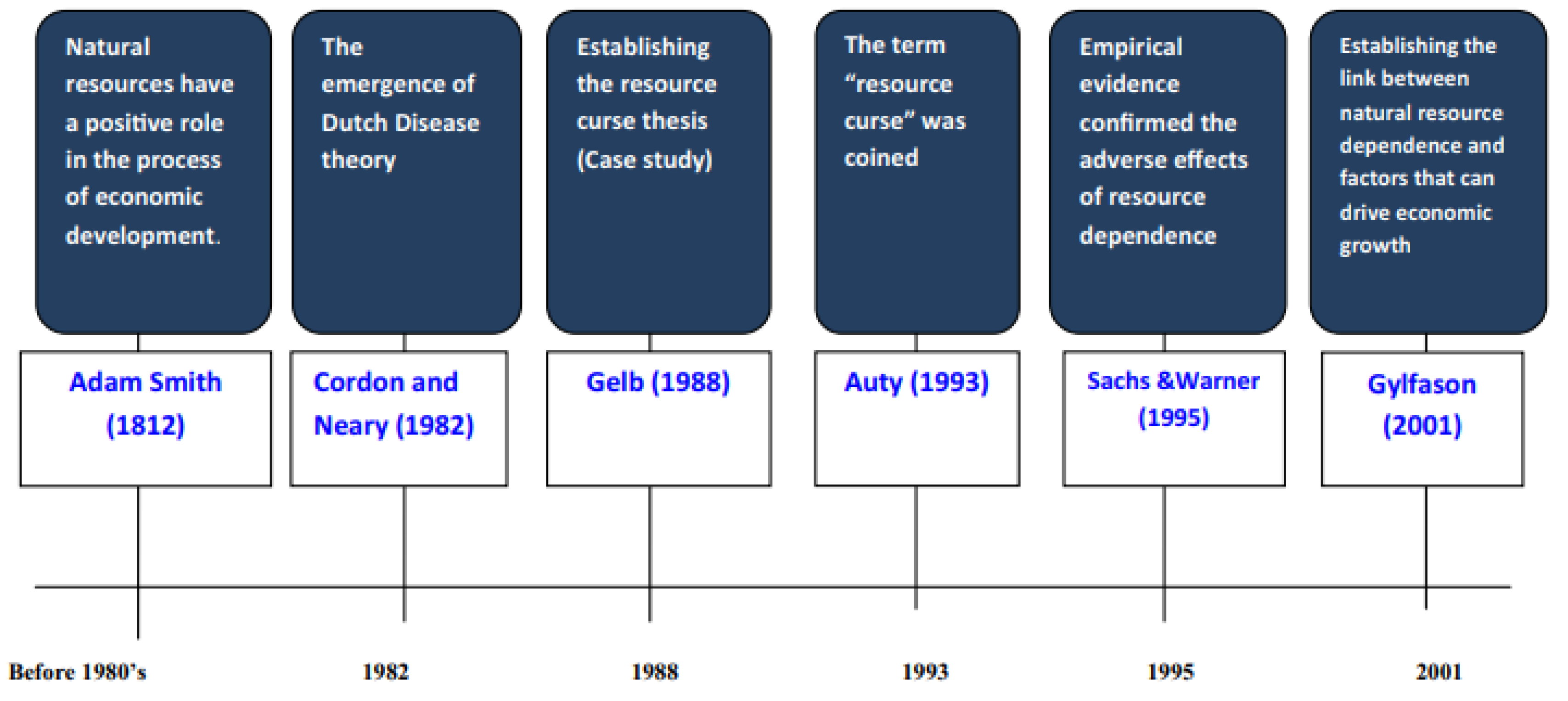
2.1.1. Short Notes of Evolution Timelines

Adam Smith argued that natural resources, in themselves, have the potential to contribute positively to economic development. He discussed the concept of “land” as one of the three factors of production, alongside labor and capital. In his view, land represented not only physical space but also the natural resources found within it, such as minerals, forests, and fertile soil. Smith believed that a nation’s wealth could be enhanced by effectively utilizing its natural resources. He emphasized the importance of efficient resource allocation and specialization of labor to increase productivity. When individuals and businesses could harness and utilize natural resources efficiently, it could lead to economic growth and development. However, it is important to note that Smith’s perspective was not an endorsement of resource extraction at any cost. He also emphasized the significance of sound institutions, free markets, and policies that promote competition and protect property rights. In his view, these factors were essential for translating the potential wealth from natural resources into actual economic development. In summary, Adam Smith’s work laid the foundation for understanding how natural resources can play a positive role in economic development, but he also emphasized the importance of good governance and market mechanisms to ensure that the benefits of these resources are realized.

The Dutch Disease theory, introduced by Corden and Neary in 1982, explains the economic challenges that can arise from a sudden resource boom. When a country experiences a surge in resource exports, its currency tends to appreciate, making other exports less competitive. This can hinder economic diversification and create vulnerability to global commodity price fluctuations. Income inequality may also increase. To address these issues, policymakers often implement strategies such as diversifying the economy and managing windfall revenues in sovereign wealth funds. The theory underscores the need for careful management of resource-driven growth to ensure long-term economic stability and development.

In 1988, Jeffrey Sachs and Andrew Warner introduced the Resource Curse thesis, highlighting that countries rich in natural resources might face economic challenges rather than benefits. This theory emphasizes: resource abundance, economic challenges of resource-rich countries, dutch disease, dependency and institutional weakness.

The term was actually coined before 1993, and it has been attributed to different scholars. While there is some debate about who first used the term, it was popularized by the publication of academic research in the 1990s. One prominent early use of the term “resource curse” is often attributed to the economist Richard Auty. Auty’s work in the late 1980s and early 1990s, particularly his book “Sustaining Development in Mineral Economies: The Resource Curse Thesis,” laid the foundation for the concept. Another influential scholar in the development of the resource curse concept is Jeffrey Sachs, who, along with Andrew Warner, published the paper “Natural Resource Abundance and Economic Growth” in 1995. This research played a significant role in bringing the concept to broader attention in the academic and policy communities.

The paper by Sachs and Warner (1995) titled “Natural Resource Abundance and Economic Growth”, played a significant role in providing empirical evidence for the adverse effects of resource dependence. In the study, Sachs and Warner examined a large dataset of countries and analyzed the relationship between natural resource abundance and economic growth. They found that countries heavily dependent on natural resource exports tended to have slower economic growth compared to countries with more diversified economies. This finding provided empirical support for the idea that an overreliance on resource exports could hinder overall economic development. This paper also highlighted the potential mechanisms through which resource dependence could negatively impact economic growth, including issues such as the Dutch Disease effect, volatile commodity prices, and governance challenges. Sachs and Warner’s research played a crucial role in bringing the resource curse concept to the forefront of academic and policy discussions, and their empirical evidence has informed subsequent studies and policy recommendations for resource-rich countries.

Thorvaldur Gylfason’s research, particularly in 2001, focused on the link between natural resource dependence and economic growth. The study emphasized several key points including resource dependence and growth, diversification, institutional factors, and social and political implications. Gylfason’s work has significantly contributed to our understanding of the challenges and opportunities faced by resource-dependent nations and has influenced policy discussions in these contexts.

2.1.2. What Happened after 2001?

After 2001, the conversation around the resources curse hypothesis has been ways to lower the negative effects the abundance of natural resources poses for economies. Researchers identified that the mechanism for the negative effects of natural resources is volatility in commodity prices (Davis and Tilton 2005; Frankel 2010; Humphreys et al. 2007), economic mismanagement (Iimi 2007; M. L. Ross 2007) rent-seeking (Bodea et al. 2016; Davis and Tilton 2005; Iimi 2007; M. Ross et al. 2011; Sala-i-Martin and Subramanian 2013) and corruption and institutional quality (Bhattacharyya and Collier 2014; Eregha and Mesagan 2016).

As a way to measure the impact of natural resources on growth, the commonly used proxy for natural resources dependence and natural resources abundance by researchers are Primary exports over GDP (Epo and Faha 2020), Rents from natural resources over GDP (Taneja et al. 2023), Share of natural capital in national wealth, Share of mineral exports in total exports (Moussa 2018), Total natural capital and mineral resource assets in US $ per capita (Canuto and Cavallari 2012) and Subsoil wealth (Badeeb et al. 2017). Different growth periods have been studied with the most recent one in 2016 by Cockx and Francken spanning 140 countries. Other control variables that have been used summarily include human capital development (Blanco and Grier 2012; Stijns 2006), savings and investment (Boos and Holm-Müller 2013; Dietz et al. 2007), openness and fiscal policy (Bornhorst et al. 2008; Papyrakis and Gerlagh 2004), export structure (Bond and Malik 2009), financial development (Bhattacharyya and Collier 2014) and spending on education (Cockx and Francken 2016).

The findings of the various studies can be grouped into two broad categories. These are grouped sample countries and single-country cases. On the grouped sample countries, (Boos and Holm-Müller 2013; Cockx and Francken 2016; Dietz et al. 2007; Papyrakis and Gerlagh 2007; Ze et al. 2023) all found a negative effect of resource abundances and resources dependence on economic growth, human capital development, saving, and investment. (Usman et al. 2023) further found that natural resources significantly increase greenhouse gas emissions and thus hurt growth. (Namahoro et al. 2023; Stijns 2006) however, found a positive effect on growth and human development.

On the single country results, a number of these studies have attributed poor economic development performance of large resource-rich nations such as Nigeria (Olayungbo 2019; Shobande 2022) the Democratic Republic of Congo (Matti 2010; Yilanci et al. 2022), Angola, Bolivia (Amundsen 2014; Andrade and Morales 2007) to the resource curse. However, some researchers have also found a positive impact of natural resources on growth (Alam et al. 2022; Li et al. 2022).

The natural resource dependence and abundance and growth hypothesis have not gone without criticism. Some of the criticism includes (1) finding no evidence of a negative effect of natural resources on growth either in cross-sectional data or panel data (Lederman et al. 2005) (2) finding in all growth periods, a negative relationship between resource dependence and economic growth in resources production sectors Alexander James (2015), (3) the resource curse hypothesis can only be determined using the correlation between resource abundance and income levels and the relationship between the two was positive (Boyce and Emery 2011) (4) oil abundance has positive effects on both income levels and economic growth (Cavalcanti et al. 2011) (5) the impact of large oil and other mineral resource is positive on long-term economic growth and (Alexeev and Conrad 2009) (6) economic growth is not affected by resource dependence and resource abundance has a positive effect on growth and institutional quality (Pendergast et al. 2011).

In the case of Ghana, some existing works have found evidence against the resources curse hypothesis (Adabor 2023; Adu 2012; Dietsche 2012) while some found it in favour (Debrah and Graham 2015). The exploration of oil in commercial quantities started in 2007 and its impact on the Ghanaian economy cannot be overlooked (Acquah-Andoh et al. 2018). Despite extensive research on Ghana’s resource curse, limited attention has been given to the role of oil in the country’s economic development. The discovery of oil in commercial quantities in Ghana in 2007 raised hopes of economic growth, but it also brought concerns about potential negative consequences. While a few studies have investigated the specific dynamics of the resource curse in Ghana post-oil discovery, the impact of oil exploration on the resource curse hypothesis requires further examination. Because of this, the inclusion of oil as a variable in the resources curse hypothesis is paramount. Some studies on the resource curse in Ghana have used oil as a variable but the focus was on its impact on agriculture (Asumadu et al. 2021). This current study thus introduces oil and assesses its impact on growth in the resource curse model. It must be noted that few works exist on the subject in the case of Ghana. This study thus improves upon other works by including oil resource data and also contributing to the evidence gap.

The hypothesis for the study Is s”own as

H₀: 

Exploration of oil affect the resource curse hypothesis position in the case of Ghana?

H₁: 

Exploration of oil affect the resource curse hypothesis position in the case of Ghana?

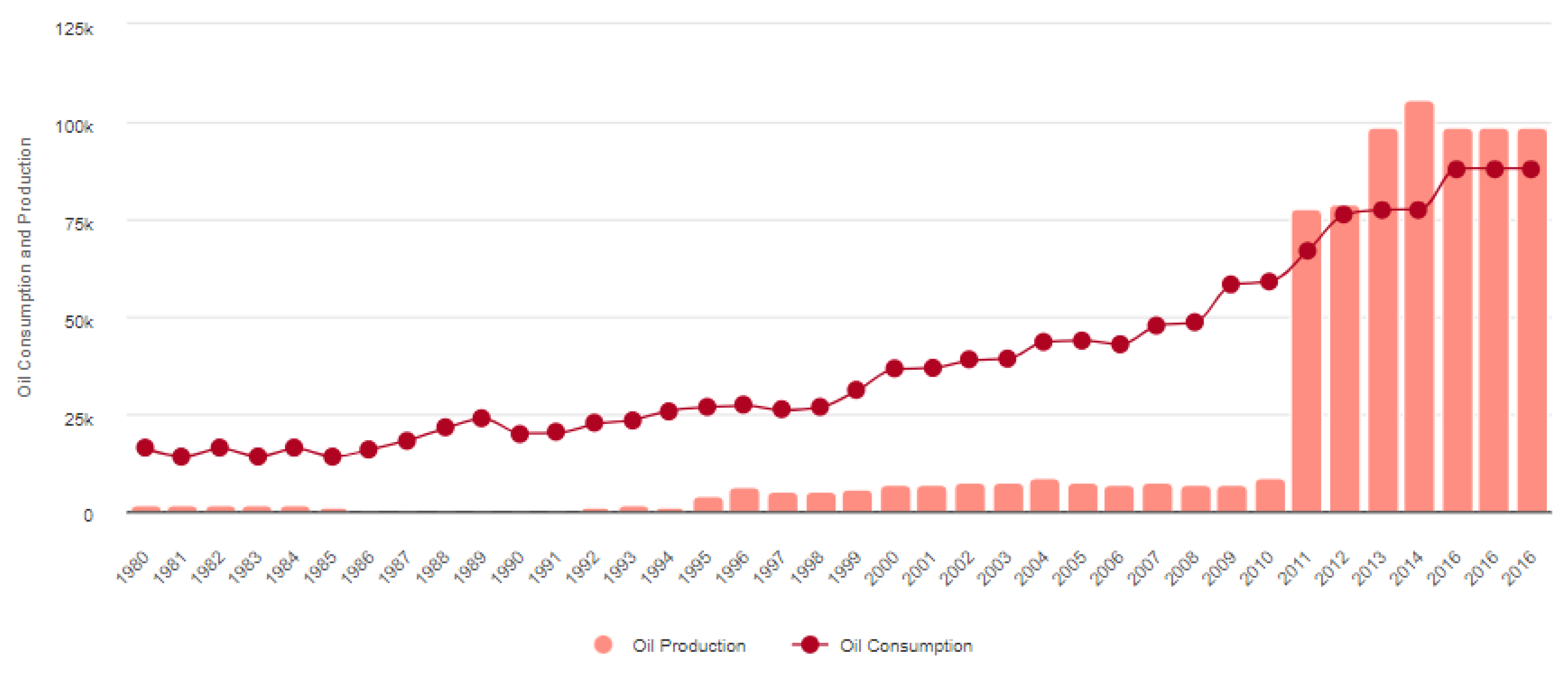
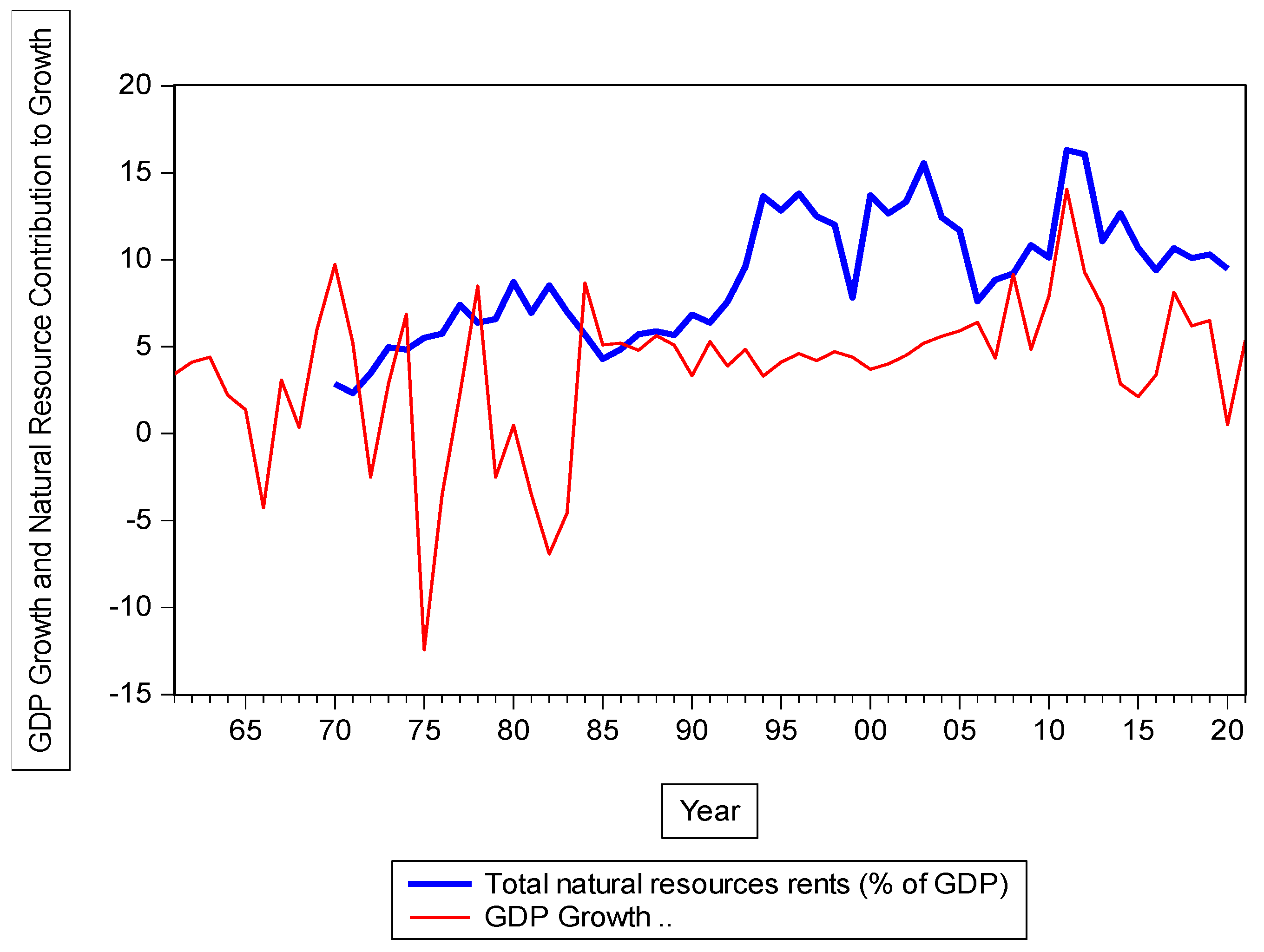
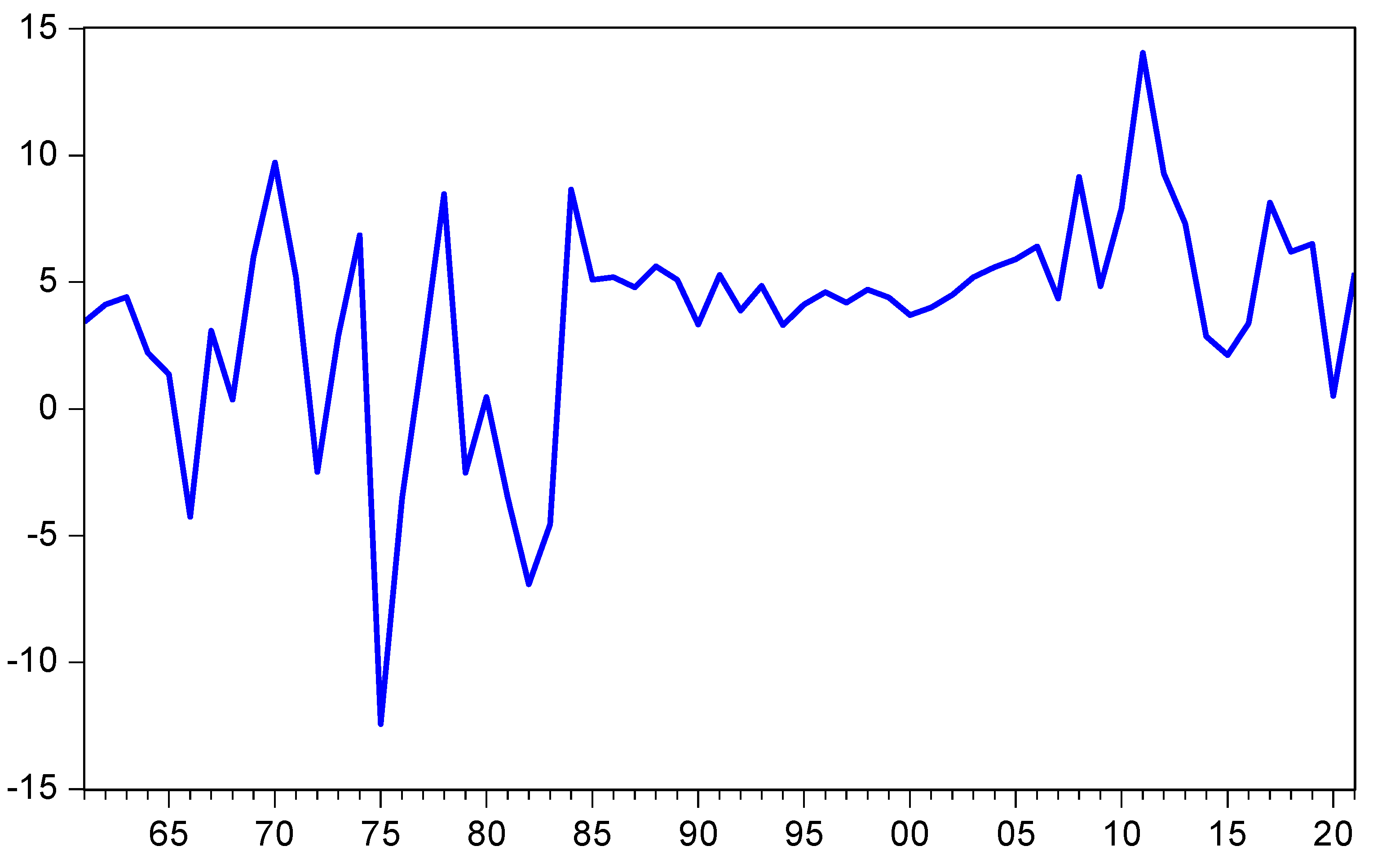
2.2. The Ghanaian Economy

The foundations of the present structure of the Ghanaian economy were laid between 1890 and 1910. This 20-year period witnessed an annual average growth of 1.8 percent in GDP per capita according to estimated national income accounts for that period. Judged by the economic performance of developing countries at that time, such a growth rate was high and marked a significant improvement in living standards (M. M. Huq 1989). The growth in GDP and the transformation of the economy continued after 1910, following the high rates of capital formation achieved in the gold-mining and cocoa sectors and also in railways and construction. Although in subsequent decades the rates of growth in these activities slowed down, per capita real GDP doubled during the half-century from 1911 to 1960, and this took place during a period of rising population (M. Huq and Tribe 2018)

The first few years of independence witnessed satisfactory rates of growth. The growth rate of real GDP was 4.6 percent in 1957, falling to 3.7 percent in 1958, but then followed by two years of substantial growth at 15.2 percent in 1959 and 7.5 percent in 1960. By the standard of developing countries, this was an exceptionally good performance and in 1960 Ghana was far ahead of many other developing countries with a per capita income (at the price levels which then applied) of £70, faring better than, for example, Nigeria (£29), Egypt (£56) and India (£25) (M. Huq and Tribe 2018).

Except for 1966, when it fell by 4.3 percent, GDP continued to grow throughout the 1960s, but the average annual real growth rate of 2.8 percent was lower than the average rate for the period before 1960. Significant fluctuations in GDP growth occurred during the 1970s with four years having negative growth rates. Between 1970 and 1980, GDP grew by only 3.7 percent (in 1970 prices), with an average annual rate of only 0.4 percent. In 1981, 1982, and 1983, GDP fell by 4.2, 6.9, and 4.6 percent, respectively (M. M. Huq 1989).

Ironically, the average per capita GDP growth rate was higher in the pre-independence period than in the late 1970s and the early 1980s as shown in Figure 3. Indeed, the average annual GDP growth of 2.8 percent during the 1960s was not negligible, but the annual population growth of 2.4 percent during this period meant an annual increase of only 0.4 percent in real GDP per capita. With the low growth rate of GDP during the 1970s and the average population growth of 2.6 percent per annum, there was a fall in real GDP per capita of 2.2 percent per annum. Significant falls in growth rates for both GDP and GDP per capita were observed during 1980–1983.

Using an index of GDP based on 1970 = 100 the level of GDP in 1957 was 63.6, rising to 75.8 in 1960 and further to 89.0 in 1965. The highest recorded level of the GDP index during this period was 112.2 in 1974, but a fall of 12.4 percent in GDP brought the index down to 98.2 in 1975. The GDP index then rose to 103.7 in 1980 but fell to less than 90 in 1983.

This historical context illuminates the nuances and resilience of Ghana’s economy, providing insights into its ability to navigate diverse economic conditions. Importantly, by juxtaposing these historical insights with our research focus, we aim to uncover the role of specific variables in steering economic growth within the Ghanaian context. This contextual understanding enables us to appreciate the potential impact of these variables, be it capital formation, resource abundance, or other determinants, on Ghana’s economic performance. The irony of higher per capita GDP growth in the pre-independence era compared to later decades, despite population growth, raises questions about the effectiveness of growth strategies and policies employed during those times. This comparative analysis serves as a stepping stone for our investigation into the determinants of economic growth and their changing roles over time. As we delve into specific factors that have influenced Ghana’s economic growth trajectory, including their positive or negative effects, the historical context informs our understanding of potential contributing factors. For instance, the robust growth achieved in certain sectors during the initial years of independence prompts a closer examination of policies that facilitated such expansion and whether similar strategies can be harnessed for sustainable growth in the present.

In essence, the Ghanaian economic backdrop offered in this literature review serves as a bridge from historical trends to contemporary research. By contextualizing the general trends within the specific focus of our study, we aim to unravel the complexities of economic growth in Ghana and offer insights that can guide policy decisions and development strategies for the future.

3. Methodology

The section outlines the empirical methods used, the various variables, and the source and description of data.

3.1. Model Specification

For model specification, the study followed (Adu 2012). The starting point of accounting for growth theoretically is the neoclassical growth model. With this model, capital and labor appear to be the main explanatory factors for a country’s growth performance. However, the model also makes room for other factors. Literature has identified some of these factors as trade openness, financial development, and government share to GDP. In the recent past concern about natural resource abundance as a determinant for growth has also come up strongly. Thus, the neoclassical growth model is augmented with an additional variable of measure of natural resource abundance.

Thus from the neoclassical growth model

$$Y_t=f\left(A,L,K,R\right)$$

(1)

where Y = real output (GDP), L = labour, K = capital, R = natural resources, A = technological progress.

By consideration, we assume technological progress as follows: financial development (FD), total government expenditure (GOVSIZE), trade openness (OPEN) defined as the degree of openness of an economy, Inflation (INFLA) as a measure of macroeconomic stability, Foreign Direct Investment (FDI) and External Debt (EXDS). Thus

$$A=g(FD, GOVSIZE, OPEN, INFLA, FDI, EXDS)$$

(2)

Substituting Equation (2) into (1)

$$\begin{array}{l}{GDP}_t\\ =F(K_t, L_t, R_t, {FD}_t, {GOVSIZE}_t, {OPEN}_t, {INFLA}_t, {FDI}_t, {EXDS}_t)\end{array}$$

(3)

From Equation (3), the operational model is expressed in log-log form as

$$\begin{array}{ll}{lnGDP}_t= {\beta }_0& +{\beta }_1{lnK}_t+{\beta }_2{lnL}_t+{\beta }_3{lnR}_t+{\beta }_4{lnFD}_t+{\beta }_5{lnGOVSIZE}_t\\ & +{\beta }_6{lnOPEN}_t+{\beta }_7{lnINFLA}_t+{\beta }_8{lnFDI}_t+{\beta }_9{lnEXDS}_t\\ & +{ϵ}_t\end{array}$$

(4)

${ϵ}_t$ is the Error term. We estimate Equation (4) using eViews 9. The expected signs for the variables are displayed in

Table 1. Expected signs of variables.

Variables	Expected Sign
Financial Development	+
Total Government expenditure	+/−
Openness	+/−
Inflation	−
Foreign Direct Investment	+
External Debt	−
Natural Resource	+

Source: Author, 2023.

below.

3.2. Times Series Estimation Techniques

Because the data used in the study are time series, we start our time series technique by performing an important diagnostic test most common for time series data: test for stationarity. The study used two tests known as the Phillips–Perron (PP) test (1988) and the Augmented Dickey–Fuller test (1976). The reason for performing this test is to determine whether the variables used are stationary or not or at what difference level these variables would be stationary. The PP test is adopted. It is based on non-parametric methods, which suffer less from distributional problems because it adjusts for serial correlation and endogeneity of the regressors so that it prevents the loss of observation (Adu 2012). Another important property of the PP test is that it is consistent even in the presence of heteroscedastic. The result of the PP test is confirmed by the ADF test.

After performing these tests, the studies proceed to choose a time series estimator that is robust and consistent in the face of the properties established about the variables. We chose the Fully Modified Ordinary Least Squares (FMOLS) estimator developed by Phillips and Hansen (1990). FMOLS models are models that account for serial correlation effects and for the endogeneity in the regressors that result from the existence of a cointegrating relationship. The FMOLS has some good properties over a wide range of time series models. Firstly the FMOLS models apply to models with either full-rank or co-integrated I(1) regressors. Under such circumstances, the limit theory of FM estimates under stationary components of the regressor is equivalent to OLS, while the FM estimates under non-stationarity components maintain their optimality properties. Secondly, FMOLS can be applied to models with stationary regressors and in this case, has the same limit theory equivalent to OLS. A case of special importance in practice is stationary autoregression (Phillips 1995a). Thirdly, FMOLS is hyper-consistent with a convergence rate that exceeds 0(T) for a unit root in autoregression (Brooks 1999). Lastly, the normal and mixed normal limit theory for the FM model helps with simple inference. This avoids problems of pre-test nuisance, parameters, overfitting, and nonstandard limit distributions that arise in other approaches (Phillips 1995b). These advantages make the FMOLS suitable over other approaches such as the ARDL (Pesaran 2004) and maximum likelihood models.

We begin by adopting the basic model by (Phillips 1995a) as follows:

$$y_t=\beta x_t+{\epsilon }_t$$

(5)

where $\beta$ is an n x w coefficient matrix and x_t is a w = (w₁ + w₂) dimensional vector of c-integrated or possibly stationary regressors specified as follows

$$P_1^{\prime }{x}_t=x_{1t}={\epsilon }_{1t} , \left(w_1\times 1\right)$$

(6)

$$P_2^{\prime }∆x_t=∆x_{2t}={\epsilon }_{2t} , \left(w_2\times 1\right)$$

(7)

Here P = $\left[P_1{P}_2\right]$ is w x w orthogonal so that the model becomes

$$y_t= {\beta }_1{x}_{1t}+{\beta }_2{x}_{2t}+{\mu }_t,$$

(8)

where ${\beta }_1=\beta P_1 and {\beta }_2=\beta P_2$

Let ${\epsilon }_t=\left({\epsilon }_{0t}^{\prime } ,{\epsilon }_{1t}^{\prime } ,{\epsilon }_{2t}^{\prime }\right) and {\phi }_t= {\epsilon }_{0t} \otimes {\epsilon }_{1t}$, it is convenient to assume that ${\epsilon }_t$ is a linear process that satisfies the error condition as follows

(a)

${\epsilon }_t= \omega \left(L\right){\mu }_t= {\sum }_{j=0}^{\infty }{\omega }_j{\mu }_{t-j} , {\sum }_0^{\infty }{j}^a\left|w_j\right|<\infty , \left|w\left(1\right)\right|\ne 0 for some a>1$

(b)

${\mu }_t is iid with zero mean, variance matrix {\sum }_e>0$ and finite fourth-order cumulants

(c)

$E\left({\phi }_{tj}\right)=E\left({\epsilon }_{t+j}⨂{ \epsilon }_{1t}\right)=0$ for all $j>0$, where ${\epsilon }_t={\epsilon }_{0t}$

This error condition assumption ensures the validity of the functional central limit theorems for ${\epsilon }_t$ and ${\epsilon }_t{\epsilon }_t^{\prime }$. We have in particular

$$n^{-1/2}{\sum }_1^{\left[n\right]}{\epsilon }_t\to dA\left(·\right)=AM \left(\upsilon \right), \upsilon =\omega \left(1\right){\sum }_e\omega \left(1\right)$$

(9)

And

$$n^{-1/2}{\sum }_1^n{\phi }_{t,0}\to dN\left(0, {\upsilon }_{\phi \phi }\right)= {\sum }_{j=-\infty }^{\infty }E \left({\epsilon }_t{\epsilon }_{t+j}^{\prime }{\otimes \epsilon }_{1t}{\epsilon }_{1t+j}^{\prime }\right)$$

(10)

The variance matrix $\sum$ and long-run variance matrix $\upsilon$ of ${\epsilon }_t$ are divided into ${\sum }_{ij}$ and ${\upsilon }_{ij} (i,j=\mathrm{0,1},2)$ conformably with ${\mu }_t$. Again we divide the Brownian motion A into Ai (i = 0, 1, 2) when ${\epsilon }_t and {\epsilon }_{1s}$ are independent for all t, s we have ${\upsilon }_{\phi \phi }={\sum }_{j=-\infty }^{\infty }E \left({\epsilon }_t{\epsilon }_{t+j}^{\prime }\right)\otimes \left({\epsilon }_1{\epsilon }_{1t+j}^{\prime }\right)$ and when in addition, ${\epsilon }_{it}=iid (0, {\sum }_{00})$ we have ${\upsilon }_{\phi \phi }={\sum }_{00}⨂{\sum }_{11}$. We also need the one-sided long-run covariance matrices

$$△= {\sum }_{j=0}^{\infty }E\left({\epsilon }_j{\epsilon }_0^{\prime }\right)= {\sum }_{j=0}^{\infty }Z\left(j\right)=\left({∆}_{ij}\right)$$

(11)

$$\forall = {\sum }_{j=1}^{\infty }E\left({\epsilon }_j{\epsilon }_0^1\right)= {\sum }_{j=1}^{\infty }Z\left(j\right)=\left({\forall }_{ij}\right)$$

(12)

where ${∆}_{ij} and {\forall }_{ij }(i,j=\mathrm{0,1},2)$ conforms to the division of the vector ${\epsilon }_t$. Both $\upsilon and \mathsf{\Delta }$ are typically estimated by kernel smoothing of the components of sample autocovariance. Since ${\epsilon }_t$ is estimated we will use in its place the residuals from a preliminary least squares on Equation (10). Under Error Condition EI), $\widehat{\beta }\to p\beta$ and the replacement of ${\epsilon }_t$ by ${\widehat{\epsilon }}_t$ will not affect our results. By replacement, we mean the asymptotic distribution of the OLS estimate with one that does not involve unit root distribution. If this assumption is relaxed, the unit root distribution of the error is non-standard, and hence carrying inference on the parameters using the t-test in OLS regression will be invalid.

Using an econometric model where the dependent variable is assumed to be I(1) and the vector of regressors is assumed to be I(1)/(0) as follows;

$$∆{\mathsf{\Gamma }}_t= {\psi }_t+{\varrho }_t$$

(13)

Equation (13) corresponds to Equation (4) in parts so that the vectors of regressors, denoted here by ${\mathsf{\Gamma }}_t$ has a first difference stationary process as shown above and ${\psi }_t$ is a kx1 vector of drift parameters and ${\varrho }_t$ is a kx1 vector of I(0) errors. As stated above non-standardization of the unit root distribution is evident in the asymptotic distribution of the OLS estimator. To overcome these problems, a correction for possible correlation between the errors in equations 13 and 4 above and their respective lagged values is required. This is where the semi-parametric Phillip–Hansen Fully Modified OLS estimator comes in handy.

3.3. Measures of Natural Resources

Various researchers have used different measures for natural resource abundance. Historically, measures of natural resources have concentrated on the share of primary commodity exports (Sachs and Warner 1995). This measure of natural resource abundance thus combines both agriculture production and extractive industry activities. (Collier 2007), however, has shown that the long-term growth effects of agriculture production are very different from non-agriculture production even though both activities fall in the primary sector. To this end, it would be important to separate these two major activities. In that case, the effects of each on economic growth could be analyzed separately.

In modern times, a measure of natural resources still includes minerals such as gold, oil (Cavalcanti et al. 2011), diamond, and a variable such as population to measure human capital (Busse and Gröning 2013; Hassan et al. 2019; Van Der Ploeg and Poelhekke 2019). Others have still focused their attention on agriculture and land mass (forestry, fishing) (Baloch et al. 2019; Fischer 2010; Alex James and Aadland 2011). While others still have a combination of human, agriculture variables and non-agriculture variables. For instance, (Sala-i-Martin and Subramanian 2013) used the share of the exports of four types of natural resources—fuel, ores and metals, agricultural raw materials, and food as a measure of resource abundance in the case of Nigeria.

Following the discussion of historical and modern measures of natural resource abundance the study selected eight variables. These are the percentage of agriculture to GDP (as a proxy for non-cash crops), total arable land, cocoa production (as a proxy for cash-crop), oil production, gold production, bauxite production, diamond production, and manganese production.

It must however be stated that Ghana has a lot of natural resources by which all resources cannot enter the model as a measure. Thus, the various measures suggested in the study are not adequate and thus are used as proxies for resource abundance. To solve this problem (Adelman and Morris 1978) suggested computing a composite index from four broad categories: namely agriculture, fuel, and non-fuel minerals. To be able to compute such an index, the study used principal component analysis. The principal components of a set of variables are obtained by computing the eigenvalues decomposition of the observed variance/correlation matrix. This would help us to derive an adequate composite index that could proxy for natural resources adequately.

Control Variable

The study included eight other control variables as suggested by (Barro 1997) in growth models. These variables are capital (as measured by gross fixed capital formation), labor (as measured by labor force participation rate), inflation, financial development (as measured by domestic credit to the private sector), foreign direct investment, trade openness (as measured by trade as a percentage of GDP), size of government (as measured by government expenditure as a percentage of GDP), and external debt.

3.4. Source of Data

Data for the study was from 1960 to 2021. Data were gathered from different sources. Data on Gold, Diamond, Manganese, and Bauxite were gathered from the Mineral Commissions and Ghana Chamber of Mines. Data on Cocoa Production were gathered from (United Nations 2022) Data on Oil was from Ghana National Petroleum Commission, 2022.

Data on the following variable: total arable land in hectors, agriculture (including forestry and fishing) as a percentage of GDP, domestic credit to the private sector as a percentage of GDP as a proxy for financial development, external debt stocks, foreign direct investment as a percentage of GDP, real GDP growth rate, gross fixed capital formation, total labor and trade as a percentage of GDP was all gathered from World Development Indicators, 2022.

4. Results and Analysis

Before proceeding with the analysis,

Table A1. Full name of variable and short form as used in the analysis.

Full Name of Variable	Short Form
Real GDP Growth rate	lnRGDP
Agriculture as a percentage of GDP	lnAgric
Total Arable Land in Hectors	lnArable
Cocoa Production (annually)	lnCocoa
Oil Production (annually)	lnOil
Gold Production (annually)	lnGold
Bauxite Production (annually)	lnBau
Diamond Production (annually)	LnDia
Mangenese Production (annually)	lnMang
Other Control Variable
Gross Fixed Capital Formation	lnCap
Total labor	lnLab
Inflation	lnInfla
Domestic Credit to private sector as a percentage of GDP as a proxy for financial development	lnFD
Foreign Direct Investment as a percentage of GDP	lnFDI
Trade as a percentage	lnOpen
Government Expenditure as a percentage of GDP	lnGovsize
External Debt Stocks	lnExds
Natural log on variable	Ln()

Source: Author’s Construct, 2023.

in the appendix shows the full name of the variable and its short form. This is executed for easy reference.

Table A2. Descriptive Analysis.

Variables	Obs	Mean	Std.Dev.	Min	Max	Skew.	Kurt.
lnOil	37	10.308	0.582	9.1	11.385	0.122	2.141
lnGold	31	14.63	0.495	13.166	15.383	−0.877	3.931
lnDiam	31	12.992	1.067	10.138	14.51	−1.282	3.887
lnBaux	31	13.335	0.407	12.732	14.206	0.357	2.056
lnMang	31	13.77	0.908	11.993	15.499	−0.222	2.174
lnCocoa	59	13.316	0.472	12.41	14.171	0.108	2.146
lnAgric	62	3.607	0.343	2.852	4.106	−0.73	2.563
lnArable	58	14.82	0.403	14.346	15.367	0.113	1.39
lnFD	61	1.995	0.669	0.433	2.894	−0.497	2.328
lnExds	51	3.829	0.572	2.805	4.938	0.257	2.008
lnFDI	49	0.214	1.502	−3.094	2.248	−0.528	2.225
lnCap	48	2.738	0.442	1.325	3.367	−0.746	3.448
lnLab	32	16.065	0.23	15.671	16.433	−0.058	1.789
lnOpen	62	3.865	0.591	1.844	4.754	−1.149	4.535
lnRGDP	62	23.559	0.654	22.759	24.915	0.72	2.18
lnInfla	60	2.988	0.799	0.663	4.813	−0.41	3.645
lnGovsize	62	2.342	0.236	1.768	2.819	−0.347	2.489

shows the summary statistics while

Table A3. Correlation Matri.

Variables	(1)	(2)	(3)	(4)	(5)	(6)	(7)	(8)	(9)	(10)	(11)	(12)	(13)	(14)	(15)	(16)	(17)
(1) lnOil	1.000
(2) lnGold	0.594	1.000
(3) lnDiam	0.039	−0.049	1.000
(4) lnBaux	0.621	0.616	0.094	1.000
(5) lnMang	0.616	0.685	0.048	0.629	1.000
(6) lnCocoa	0.590	0.789	−0.111	0.695	0.837	1.000
(7) lnAgric	−0.603	−0.780	0.210	−0.656	−0.673	−0.804	1.000
(8) lnArable	0.609	0.923	−0.084	0.689	0.798	0.864	−0.786	1.000
(9) lnFD	0.604	0.927	−0.102	0.593	0.788	0.839	−0.727	0.967	1.000
(10) lnExds	−0.389	−0.447	0.068	−0.553	−0.616	−0.632	0.667	−0.569	−0.471	1.000
(11) lnFDI	0.464	0.788	−0.218	0.485	0.517	0.694	−0.774	0.707	0.701	−0.642	1.000
(12) lnCap	0.322	0.091	0.282	0.161	0.026	0.061	−0.033	0.000	0.054	0.408	−0.100	1.000
(13) lnlab	0.682	0.880	−0.186	0.728	0.839	0.931	−0.913	0.933	0.899	−0.690	0.772	0.011	1.000
(14) lnOpen	0.125	0.550	−0.036	0.033	0.271	0.279	−0.067	0.497	0.592	0.294	0.210	0.312	0.266	1.000
(15) lnRGDP	0.667	0.839	−0.219	0.692	0.805	0.911	−0.948	0.891	0.849	−0.692	0.758	−0.000	0.989	0.183	1.000
(16) lnInfla	0.015	−0.071	0.428	0.073	−0.074	−0.187	0.043	−0.173	−0.272	0.047	−0.043	0.336	−0.162	−0.122	−0.166	1.000
(17) lnGovsize	−0.660	−0.452	0.083	−0.647	−0.418	−0.382	0.522	−0.562	−0.455	0.528	−0.424	0.147	−0.560	0.127	−0.546	0.001	1.000

shows the correlation matrix. The variable of interest lnOil has a mean of approximately 10.308 with a standard deviation of 0.582. It has a relatively small spread, as indicated by the narrow range between the minimum (9.1) and maximum (11.385) values. The skewness is positive (0.122), suggesting a slight rightward skew in the data. The kurtosis (2.141) indicates that the distribution has relatively heavier tails compared to a normal distribution. For FMOLS, these statistics suggest that lnOil may have a relatively stable and normally distributed pattern. With lnGold a mean of approximately 14.63 and a standard deviation of 0.495, means it has a moderate spread. The skewness is negative (−0.877), indicating a leftward skew in the data. The kurtosis (3.931) suggests heavy tails and potential outliers. For FMOLS, these statistics suggest that lnGold may have a distribution that deviates from normality and could require further examination for potential outliers. The variable lnDiam has a mean of approximately 12.992 and a relatively high standard deviation of 1.067, indicating a wider spread. The skewness is negative (−1.282), suggesting a leftward skew and the kurtosis (3.887) indicates heavy-tailedness. Similar to lnGold, lnDiam may deviate from normality. With lnBaux a mean of approximately 13.335 and a standard deviation of 0.407, indicate it has a narrower spread. The skewness is positive (0.357), and the kurtosis (2.056) suggests moderately heavy tails. For FMOLS, these statistics indicate that lnBaux may have a relatively stable and normally distributed pattern. This variable (lnMang) has a mean of approximately 13.77 and a standard deviation of 0.908, indicating a wider spread. The skewness is slightly negative (−0.222), and the kurtosis (2.174) suggests moderate tail heaviness. lnMang may require examination for potential outliers in FMOLS. lnCocoa has a mean of approximately 13.316 and a standard deviation of 0.472. Its skewness is close to zero (0.108), and the kurtosis (2.146) suggests a moderately heavy-tailed distribution. lnCocoa may be relatively normally distributed and suitable for FMOLS. lnAgric has a mean of approximately 3.607 and a standard deviation of 0.343. It has a relatively narrow spread. The skewness is negative (−0.73), indicating a leftward skew and the kurtosis (2.563) suggests moderately heavy tails. For FMOLS, these statistics suggest that lnAgric may deviate from normality and require further examination.

4.1. Diagnostic Test

Unit Root

Before proceeding to the analysis, the study first tests the stationary or otherwise of the variables used. The two main tests as discussed earlier are the Phillips–Perron (PP) test (1988) which is consistent with small samples and the Augmented Dickey–Fuller test (1976). The test of unit root at the level by the ADF in

Table 2. Results of ADF and PP unit root test by levels (log levels) and by first difference.

PART A			PART B
Series	ADF (Probability)	PP (Probability)	Series	ADF (Probability)	PP (Probability)
LNRGDP	1.0000	1.0000	D(LNRGDP)	0.0001 ***	0.0001 ***
LNOPEN	0.4952	0.4455	D(LNOPEN)	0.0000 ***	0.0000 ***
LNOIL	0.1496	0.2650	D(LNOIL)	0.0000 ***	0.0001 ***
LNMANG	0.7315	0.7014	D(LNMANG)	0.0011 **	0.0014 **
LNLAB	0.0090 **	0.0523	D(LNLAB)	0.0085 **	0.0085 **
LNINFLA	0.0055 **	0.0102	D(LNINFLA)	0.0000 ***	0.0000 ***
LNGOVSIZE	0.0464 *	0.0341	D(LNGOVSIZE)	0.0000 ***	0.0000 ***
LNGOLD	0.0093 **	0.0064 **	D(LNGOLD)	0.0000 ***	0.0000 ***
LNFDI	0.5537	0.5651	D(LNFDI)	0.0000 ***	0.0000 ***
LNFD	0.6756	0.6480	D(LNFD)	0.0000 ***	0.0000 ***
LNEXDS	0.4457	0.3536	D(LNEXDS)	0.0000 ***	0.0000 ***
LNDIA	0.9425	0.9706	D(LNDIA)	0.0006 ***	0.0008 **
LNCOCOA	0.7551	0.8239	D(LNCOCOA)	0.0000 ***	0.0000 ***
LNCAP	0.0045	0.0049 **	D(LNCAP)	0.0000 ***	0.0000 ***
LNBAU	0.5554	0.7193	D(LNBAU)	0.0001 ***	0.0000 ***
LNARABLE	0.9647	0.9485	D(LNARABLE)	0.0000 ***	0.0000 ***
LNAGRIC	0.9923	0.9493	D(LNAGRIC)	0.0000 ***	0.0000 ***

Note: ***, **, * indicate significance at 1%, 5%, and 10%. Source: Authors Calculation, 2023.

Part A shows that only labor, inflation, government size, and gold variables were stationary. The rest of the variables were not stationary. The results of the PP test also in Table 2 Part A showed that gold and capital were stationary. The rest of the variables were not stationary. The implication of this is that shocks to any of the non-stationary variables will have a permanent effect. There is thus an absence of a mean reverting process in all the variables we tested but for the stationary ones.

The quick test of stationarity of the variable at first difference reveals that all variables were stationary. The results are shown in Table 2 Part B. The presence of unit roots justifies the choice for the fully modified ordinary least square approaches which corrects for both non-stationarity and endogeneity as proved by Phillips and Hansen (1990).

4.2. Results and Discussions

The results of Fully Modified OLS are presented in

Table 3. FMOLS Regression Result: Dependent Variable: Log of real GDP (lnRGDP).

Variables	Coefficients
	Model 1	Model 2	Model 3	Model 4
Indicators of Abundance of Resources
lnAgric	0.2441 ***	0.3380 ***	0.3866 ***
lnArable	0.3848	0.2134 *		0.0981 ***
lnCocoa	−0.0602	0.0378 **		0.0207 **
lnOil	0.0112 **	0.0005	−0.0124
lnGold	0.0530 **		0.0415 *
lnBau	−0.1096 *	−0.1017	−0.0142 **
LnDia	0.0094 **	0.0186	0.0204
lnMang	−0.0068	−0.0128	0.3925 **
Other Control Variable
lnCap	0.0106 **	0.0192 *	0.0105 **	0.0568 **
lnLab	0.4992 ***	0.4302 ***	0.0716 ***	0.9999 ***
lnInfla	−0.0132**	−0.0368 **	−0.0059	0.0001
lnFD	−0.1126**	−0.1236 *	−0.0021	0.0629
lnFDI	0.1452**	0.3547 **	0.2575 ***	0.0245 **
lnOpen	−0.1954 ***	0.0096	−0.2002 **	−0.1572 **
lnGovsize	−0.1018	−0.0058 *	0.0180	0.0815
lnExds	−0.0694 ***	−0.050 **	−0.0723 **	−0.0395 **
Constant	−1.5282 ***	−1.0269 ***	−1.687 ***	−4.6028

Note: ***, **, * indicate significance at 1%, 5%, and 10%. Source: Authors Calculation, 2023.

below.

Four models were estimated. Model 1 included all the variables used, in Model 3, we dropped all agriculture-related measures while in Model 4 we dropped all non-agricultural-related measures. In Model 3, the gold production variable was dropped to check the effect of illegal mining on the availability of arable land.

On the issues of natural resource abundance, all four models featured the proxies for natural resource abundance. Agricultural as a percentage of GDP (lnAgric) was positive and statistically significant at a one percent level in Models 2 and 3. This showed that agricultural productivity as a natural resource affects growth. This is in line with (Moshiri and Hayati 2017) and (Mavrotas et al. 2011) even though these researchers acknowledge the need for better institutional quality. More capital investment would ensure much higher growth. This is the only way the country can ensure sustainable growth through agriculture. The current system of traditional farming has outlived its usefulness. Total arable land (lnarable) is statistically significant in Models 2 and 4. Normally, researchers are not likely to think of arable land as a natural resource. The concentration has been on mineral resources, but this study has proved otherwise (Moyo 2009a, 2009b). However, it is instructive to note that the co-efficient of arable land is not statistically significant in Model 1. A cursory look at the other variables shows that lngold is significant. A simple inference from this shows the effects of activities that reduce the availability of arable land such as illegal mining. Illegal mining, also known as artisanal and small-scale mining (ASM), can significantly diminish the productivity of arable land through various means. These activities lead to land degradation, compromising soil fertility and structure, and often introducing harmful pollutants such as mercury and cyanide. Deforestation associated with illegal mining contributes to soil erosion and reduced land capacity for crop cultivation. Miners encroach upon agricultural lands, displacing farmers and disrupting farming activities. Water resources, crucial for irrigation, are often depleted or contaminated. Conflicts over mining resources can create insecurity, discouraging farming and displacing communities. Additionally, the loss of biodiversity and the regulatory challenges associated with illegal mining further exacerbate its negative impacts on arable land, posing a substantial threat to food security and local livelihoods in affected areas. Thus, with ongoing illegal mining activities, there is the destruction of arable land and therefore, the insignificance of the variable in Model 1. The same explanation could also be given to the lncocoa variable. The negative effect of such activities has been emphasized by (Boakye 2020; Laari 2018; Osman et al. 2022; Wedam et al. 2014)

Gold and Diamond production (lngold and India) variables showed a positive and significant effect. The significance is shown in Model 1 for both and Model 3 for only gold. The revenue generation for gold and its impact on growth transcends every aspect of the economy on both the micro and macro levels. Bauxite production, however (lnbau) showed a negative effect on growth. This agrees with Adu (2012).

On the signs and significance of the other control variables, all the variables had the expected signs except lnFD and lnOpen. The log of capital (lnCap) and log of labor (lnlab) were statistically significant in all the models. Using neoclassical growth theory, the coefficient of both variables was within the expected growth rate. Basically, from all the models, the elasticity of output concerning labor was larger than the elasticity of output concerning capital. This result is consistent with (Faggian et al. 2019; Pelinescu 2015; Teixeira and Queirós 2016). The Financial Development (lnFD) variable was negative and statistically significant for Models 1 and 2. This is contrary to theory and other empirical works. Theoretically, the sign for financial development should be positive but the variable in the Model is negative. This may be a result of high-interest charges on domestic funds. Such a high rate tends to hurt domestic credit to the private sector.

LnInfla has the expected sign in three models indicating the negative impact of inflation on economic growth. Foreign direct investment (lnFDI) has a positive impact on growth as also suggested by other researchers. External debt (lnExds) harmed growth. Trade openness (lnOpen) has a positive impact on growth. The size of the government (lnGovsize) is negative and statistically significant in Model 2. These results support the crowding-out effect of government spending.

Oil Production (lnOil) is statistically significant in Model 1. This shows the positive effect of oil as a natural resource on economic growth. Since the beginning of the extraction of oil in commercial quantities, the government has gained $464 million, $938 million, and $343 million in terms of revenue in 2018, 2019, and 2020 (Kwarteng 2022). These data underscores the economic significance of oil production as a revenue source for the government. Ghana’s economic growth rate with oil was 4.3 percent in 2020 while growth without oil was 0.5 percent for the same year. This comparison demonstrates the contribution of oil production to overall economic growth in that year. In all, Ghana has earned about 6 billion dollars in oil revenue for the past ten years. This revenue has since been invested in areas such as Annual Budget Funding Amount (ABFA)—$2.6 billion (40 percent) over the period, Ghana National Petroleum Cooperation (GNPC), $2.0 billion (30 percent), the Ghana Stabilisation Fund (GSF), $1.39 billion (21 percent), and the Ghana Heritage Fund (GHF), $586 million (9 percent) (Kwarteng 2022).

To compare the results of oil with other natural resources in the study, let’s analyze the coefficients and significance levels of the oil variable (lnOil) alongside other natural resource variables (lngold, lnbau, lndia, lncocoa, lnarable, lnmang) across the four models (Model 1, Model 2, Model 3, and Model 4)

• lnOil (Oil Production):

In Model 1: The coefficient for lnOil is positive and statistically significant at the 1% level, indicating that oil production has a significant positive impact on economic growth in the presence of all other variables.

In Model 2: The coefficient for lnOil is not statistically significant, meaning that when we exclude agriculture-related measures, the impact of oil production on growth is not statistically distinguishable from zero.

In Model 3: The coefficient for lnOil is negative and statistically significant at the 5% level. In this model, we exclude all non-agriculture-related measures, and the negative coefficient suggests that oil production might have a detrimental effect on growth when considered in isolation.

In Model 4: The coefficient for lnOil is not statistically significant, similar to Model 2. When we include only agriculture-related measures, the impact of oil production on growth is not statistically significant.

2.

Other Natural Resource Variables:

lngold (Gold Production): lngold shows a positive and statistically significant impact on growth in Model 1 and Model 3, but it becomes statistically insignificant in Model 2 and Model 4. This suggests that the significance of gold production’s impact on growth depends on the presence of other variables.

lnbau (Bauxite Production): lnbau shows a negative impact on growth in Model 1 and Model 3, but it becomes statistically insignificant in Model 2 and Model 4. Similar to gold production, the significance of bauxite production’s impact on growth depends on the presence of other variables.

lndia (Diamond Production): lndia is not statistically significant in any of the models, indicating that diamond production does not have a significant impact on economic growth in this study.

lncocoa (Cocoa Production): lncocoa is statistically significant in Models 2 and 3, but not in Models 1 and 4. This suggests that cocoa production’s impact on growth depends on the presence of agriculture-related measures.

lnarable (Total Arable Land): lnarable is statistically significant in Models 2 and 4, but not in Models 1 and 3. This indicates that the significance of total arable land’s impact on growth depends on the presence of other variables.

lnmang (Manganese Production): lnmang is not statistically significant in any of the models, suggesting that manganese production does not have a significant impact on economic growth in this study.

Overall, the results show that the impact of oil production on economic growth is sensitive to the inclusion or exclusion of other variables in the model. In Model 1, where all variables are included, oil production has a significant positive impact on growth. However, in Models 2 and 4, where either agriculture-related or non-agriculture-related measures are excluded, the impact of oil production becomes statistically insignificant or even negative in Model 3.

The implication of the statement is that the relationship between oil production and economic growth is complex and dependent on the presence of other variables in the model. The results suggest that when all relevant variables are included (Model 1), oil production has a significant positive impact on economic growth. However, when certain variables are excluded (Models 2 and 4), particularly those related to agriculture or non-agriculture measures, the impact of oil production becomes statistically insignificant or even negative in Model 3. This sensitivity to the inclusion or exclusion of other variables indicates that the relationship between oil production and economic growth is influenced by various factors. These factors could include the role of other industries, government policies, international economic conditions, and the overall economic structure of Ghana.

The results highlight the importance of considering a comprehensive set of variables when studying the impact of oil production on economic growth. Simply focusing on oil production alone may not provide an accurate understanding of the relationship, as it interacts with other economic factors. Researchers and policymakers should be cautious about drawing definitive conclusions about the impact of oil production on economic growth without considering the broader context and potential confounding variables. Further analysis and understanding of these interactions are crucial for making informed decisions and policies related to oil production and its effects on the economy.

4.3. Hypothesis Testing—Further Explanations Using Principal Component Analysis

We explore further explanations for natural resource variables using the principal component analysis. The result is presented in

Table 4. FMOLS with composite indicators of Resources Abundance.

Variables	Coefficient	Prob.
Composite Indicators
P1	0.0214	0.049
P2	0.0318	0.002
P3	0.0951	0.010
P4	0.0125	0.040
Control Variables
lnCap	0.0015	0.001
lnLab	0.3145	0.000
lnInfla	−0.0014	0.032
lnFD	−0.0054	0.041
lnFDI	0.0029	0.005
lnOpen	0.0245	0.009
lnGovsize	−0.0235	0.038
lnExds	−0.0458	0.017
Constant	3.5146	0.000

Source: Authors Calculation, 2023.

below. From the table, we aggregate the various proxies into four main groups. The first group is known as P1 and it is made up of cocoa production (0.403), arable land (0.410), and share of agriculture (0.483). Together this component accounts for 65% of the total variance of the original data. The second component P2 is diamond (0.933). The third component, P3 is oil production (0.782) and bauxite (−0.416). The fourth component is gold production (0.571) and manganese (0.677). All these four components explain 91% of the total variance in the original data, hence these are an adequate representation of the data.

All resource abundance composites namely P1, P2, P3, and P4 had a positive sign even though some individual variables in the components showed a negative sign. On the first composite (P1) index share of agriculture, arable land, and cocoa production, there was a positive impact on growth. This thus defects the resources curse theory. On the second component (P2), the composite also showed a positive impact on growth. The third (P3) now presents us with a challenge. This is because while one of the variables has a negative impact the other has a positive impact. To determine their individual effects, we consider the following equation

$$\frac{\partial lnY}{\partial ln{P}_3}= +\frac{\partial lnY}{\partial P_3}\frac{\partial P_3}{\partial lnOil}-\frac{\partial lnY}{\partial P_3}\frac{\partial P_3}{\partial lnBau}$$

(14)

Equation (14) shows that while oil production has a positive impact on growth, bauxite production has a negative impact. However, the impact of oil production far outweighs that of bauxite production. This may be the reason for the positive sign for P3 components. Because of this positive impact, the resource curse theory is also not supported. This finding does not agree with (Satti et al. 2014; Tiba 2019; Shahbaz et al. 2019) but agrees with (Olayungbo 2019). Let’s break down the information related to P3. This is shown by the eigen value, proportion of total variance and cumulative proportion in

Table 5. Principal Components Analysis. Principal Components/Correlation.

	Component	Eigenvalue		Difference		Proportion		Cumulative
Number of Obs = 26	Comp1	5.272		4.179		0.659		0.659
Number of Comp = 8	Comp2	1.093		0.576		0.137		0.796
Trace = 8	Comp3	0.517		0.141		0.065		0.860
Rho = 1.000	Comp4	0.377		0.025		0.047		0.907
	Comp5	0.352		0.128		0.044		0.952
	Comp6	0.224		0.110		0.028		0.979
	Comp7	0.114		0.063		0.014		0.994
	Comp8	0.051		.		0.006		1.000
Variable	Comp1	Comp2	Comp3	Comp4	Comp5	Comp6	Comp7	Comp8	Unexplained
lnoil	0.327	0.162	0.782	0.475	−0.102	0.047	0.124	−0.045	0
lngold	0.389	−0.042	0.291	0.548	−0.171	0.251	−0.053	0.590	0
India	−0.027	0.933	0.223	0.033	−0.141	−0.220	0.069	−0.071	0
lnbau	0.349	0.204	−0.416	−0.799	0.086	0.261	−0.113	0.102	0
lnmang	0.377	0.113	0.183	0.291	0.677	0.013	−0.476	0.203	0
lncocoa	0.403	−0.073	0.210	−0.037	0.311	−0.110	0.821	0.055	0
lnagric	−0.483	0.198	0.022	0.149	0.223	0.825	0.227	0.102	0
lnarable	0.410	−0.051	0.276	0.071	−0.178	0.354	−0.107	−0.761	0

Principal components (eigenvectors). Source: Authors Calculation, 2023.

.

Eigenvalue (0.517): The eigenvalue represents the amount of variance explained by the corresponding principal component. In this case, P3 has an eigenvalue of 0.517. A higher eigenvalue indicates that the component explains more variance in the data. In terms of explaining economic growth in Ghana, this eigenvalue suggests that P3 captures a moderate amount of variance related to economic growth and potentially other associated variables.

Proportion of Total Variance (6.5%): The proportion of total variance explains how much of the overall variability in the original data are accounted for by the specific principal component. In this case, P3 explains approximately 6.5% of the total variance. Regarding economic growth, this means that P3 contributes to explaining a relatively small portion of the variability in economic growth and potentially other relevant factors.

Cumulative Proportion (86.0%): The cumulative proportion represents the cumulative amount of variance explained by the principal components up to the component in question. In this case, the cumulative proportion of 0.860 indicates that the first three principal components (Comp1, Comp2, and Comp3) together explain 86.0% of the total variance. This suggests that a significant portion of the variability in economic growth, including associated factors, is captured by these three components.

In summary, regarding the explanation of economic growth in Ghana, Component 3 (P3) captures a moderate amount of variance related to economic growth and potentially other relevant factors. While P3 may not explain a large portion of the total variability in economic growth on its own, it contributes to the broader understanding of patterns and relationships within the dataset. The fact that the first three components together explain a substantial portion (86.0%) of the total variance indicates the importance of these components in describing the variability in economic growth and other relevant factors.

Component P4 which is also made up of gold and manganese production also has a positive impact on growth.

Here are some potential reasons why Ghana might have managed to avoid the resource curse in the context of oil production. Firstly, Ghana has made efforts to diversify its economy away from over-reliance on oil. The government has actively promoted the development of other sectors, such as agriculture, and services to reduce the country’s vulnerability to fluctuations in oil prices and revenues. Secondly, Ghana has undertaken institutional reforms to enhance transparency, accountability, and governance in the oil sector. The government established the Public Interest and Accountability Committee (PIAC) to monitor and oversee the management of oil revenues, ensuring that they are used for the benefit of the nation and not subject to misuse or corruption. Thirdly, Ghana created the Petroleum Holding Fund, which functions as a sovereign wealth fund to save and invest a portion of oil revenues for future generations. This fund serves as a buffer against oil price volatility and helps to prevent overconsumption of oil revenues. Fourthly, rather than relying solely on oil revenues for immediate consumption, Ghana has channeled some of the oil proceeds into infrastructure development and human capital investment (Free Senior High School). This includes investments in education, healthcare, and skills development, which can contribute to long-term economic growth and development. Again, Ghana has managed its oil production in a phased and gradual manner, allowing for a smoother integration of oil revenues into the economy. This approach helps to avoid sudden and excessive inflows of revenue, which can lead to macroeconomic imbalances and other challenges associated with the resource curse. From Figure 4 oil production has smoothen from 2011 to 2016.

Lastly, Ghana has been mindful of the experiences of other oil-producing nations, both positive and negative, and has sought to learn from their successes and mistakes. This has enabled the country to adopt best practices and avoid potential pitfalls.

It is essential to recognize that the absence of the resource curse in the case of oil in Ghana is not guaranteed indefinitely. Maintaining effective governance, managing oil revenues responsibly, and continually diversifying the economy will remain crucial in ensuring that Ghana continues to benefit from its oil resources without succumbing to the negative effects often associated with the resource curse. Ongoing commitment to good governance, transparency, and sustainable development will be vital for Ghana’s long-term success in managing its oil wealth.

The main limitations of the study include data limitations that are the availability and quality of historical data, especially for the period before 1960, which may present constraints on the accuracy and completeness of our analysis, and methodological limitations: while the FMOLS regression approach was employed to estimate relationships between variables, it is important to acknowledge that no model can capture all complexities of real-world dynamics. The chosen model may have its own assumptions and limitations that could affect the robustness of our conclusions and generalizability.

Future studies could benefit from efforts to enhance the availability and accuracy of historical data, especially for the pre-1960 period. Collaborations with archival institutions, data digitization initiatives, and meticulous data validation procedures could contribute to more comprehensive and reliable datasets. Future research could consider a broader array of variables, including social, political, and institutional factors, to provide a more comprehensive understanding of the drivers of economic growth. This might involve exploring factors such as governance quality, technological advancements, and income distribution.

5. Conclusions

In conclusion, this study offers a comprehensive exploration of the intricate interplay between natural resource abundance and economic growth in Ghana, with a particular focus on the role of oil production using data from 1960 to 2021. By employing the robust Fully Modified OLS methodology, the study underlines the importance of including oil as a crucial variable in understanding economic growth dynamics. Contrary to conventional resource curse theory, the positive impact of oil production on growth is evident, especially when considered alongside a comprehensive set of variables. This finding challenges simplistic notions of a resource curse and highlights the necessity of considering the broader economic context. Moreover, the study demonstrates the value of advanced analytical tools such as Principal Component Analysis, revealing the intricate relationships within the dataset. Ghana’s success in avoiding the resource curse can be attributed to its multifaceted approach, including diversified economic strategies, transparent governance, and responsible revenue management. It is imperative to emphasize that the inclusion of oil as a significant factor in this analysis is justified by its tangible contributions to economic growth. The positive effects observed underscore the potential benefits of harnessing oil resources while maintaining a holistic view of the overall economic landscape. Looking ahead, the study’s insights provide valuable guidance for policymakers in resource-rich nations, illustrating how prudent management and strategic utilization of key resources, such as oil, can lead to resilient and inclusive economic growth. Ghana’s experience serves as a compelling example of how thoughtful policy decisions can mitigate potential pitfalls and enable long-term prosperity.

6. Policy Implication

Policy implications for the study can be grouped into short-term, medium-term, and long-term policy. The short policy has to do with augmenting agriculture productivity as agriculture has a positive impact on growth. This could be executed through specific government policies such as planting for food and jobs and more capital investment. Arable land was revealed to have been a valuable natural resource and should be protected from future destruction. In the medium term, cocoa production should be given a second look because the destruction of arable land tends to affect it. There should be a deliberate government policy to increase the production of cocoa through mechanization. In the long term, oil production should be considered an important mainstay of the Ghanaian economy. Due to this, any legal/administrative framework needed to protect leakages of oil revenue should be tightened firmly.

References

1. Acquah-Andoh, Elijah, Denis M. Gyeyir, David M. Aanye, and Augustine Ifelebuegu. 2018. Oil and Gas Production and the Growth of Ghana’s Economy: An Initial Assessment. International Journal of Economics & Financial Research 4: 303–12. [Google Scholar]
2. Adabor, Opoku. 2023. Averting the ‘Resource Curse Phenomenon’ through Government Effectiveness. Evidence from Ghana’s Natural Gas Production. Management of Environmental Quality: An International Journal 34: 159–76. [Google Scholar] [CrossRef]
3. Adelman, Irma, and Cynthia Taft Morris. 1978. Growth and Improverishment in the Middle of the Nineteenth Century. World Development 6: 245–73. [Google Scholar] [CrossRef]
4. Adu, George. 2012. Studies on Economic Growth and Inflation. Uppsala: Pub.epsilon.slu.se, vol. 2012, p. 14. [Google Scholar]
5. Alam, Md Shabbir, Tomiwa Sunday Adebayo, Radwa Radwan Said, Naushad Alam, Cosimo Magazzino, and Uzma Khan. 2022. Asymmetric impacts of natural gas consumption on renewable energy and economic growth in Kingdom of Saudi Arabia and the United Arab Emirates. Energy & Environment. [Google Scholar] [CrossRef]
6. Alexeev, Michael, and Robert Conrad. 2009. The Elusive Curse of Oil. The Review of Economics and Statistics 91: 586–98. [Google Scholar] [CrossRef]
7. Amundsen, Inge. 2014. Drowning in Oil: Angola’s Institutions and the ‘Resource Curse’. Comparative Politics 46: 169–89. [Google Scholar] [CrossRef]
8. Andrade, Saraly, and Joaquin Morales. 2007. Institute for Advanced Development Studies. Available online: https://econpapers.repec.org/paper/advwpaper/200711.htm (accessed on 4 September 2023).
9. An, Min, Ping Xie, Weijun He, Bei Wang, Jin Huang, and Ribesh Khanal. 2022. Spatiotemporal Change of Ecologic Environment Quality and Human Interaction Factors in Three Gorges Ecologic Economic Corridor, Based on RSEI. Ecological Indicators 141: 109090. [Google Scholar] [CrossRef]
10. Asumadu, George, Daniel Ofori, John Agyei, and Ali Yahuza Bawa. 2021. Ghana’s Oil Discovery and Natural Resource Curse Nexus. Modern Economy 12: 1959–71. [Google Scholar] [CrossRef]
11. Auty, Richard. 2002. Sustaining Development in Mineral Economies: The Resource Curse Thesis. London: Routledge. [Google Scholar]
12. Badeeb, Ramez Abubakr, Hooi Hooi Lean, and Jeremy Clark. 2017. The Evolution of the Natural Resource Curse Thesis: A Critical Literature Survey. Resources Policy 51: 123–34. [Google Scholar] [CrossRef]
13. Baloch, Muhammad Awais, Nasir Mahmood, and Jian Wu Zhang. 2019. Effect of Natural Resources, Renewable Energy and Economic Development on CO2 Emissions in BRICS Countries. Science of the Total Environment 678: 632–38. [Google Scholar]
14. Barro, Robert J. 1997. Determinants of Economic Growth: A Cross-Country Empirical Study. In Lionel Robbins Lectures. Cambridge: MIT Press. [Google Scholar]
15. Bhattacharyya, Sambit, and Paul Collier. 2014. Public Capital in Resource Rich Economies: Is There a Curse? Oxford Economic Papers 66: 1–24. [Google Scholar] [CrossRef]
16. Blanco, Luisa, and Robin Grier. 2012. Natural Resource Dependence and the Accumulation of Physical and Human Capital in Latin America. Resources Policy 37: 281–95. [Google Scholar] [CrossRef]
17. Boakye, Richard. 2020. Assessment of the Effects of Illegal Small-Scale Mining on Cocoa Farming and Livelihood Birim North District. Ph.D. thesis, University of Cape Coast Repository, Cape Coast, Ghana. [Google Scholar]
18. Bodea, Cristina, Masaaki Higashijima, and Raju Jan Singh. 2016. Oil and Civil Conflict: Can Public Spending Have a Mitigation Effect? World Development 78: 1–12. [Google Scholar] [CrossRef]
19. Bond, Stephen R., and Adeel Malik. 2009. Natural Resources, Export Structure, and Investment. Oxford Economic Papers 61: 675–702. [Google Scholar] [CrossRef]
20. Boos, Adrian, and Karin Holm-Müller. 2013. The Relationship between the Resource Curse and Genuine Savings: Empirical Evidence. Journal of Sustainable Development 6: 59. [Google Scholar] [CrossRef]
21. Bornhorst, Fabian, Sanjeev Gupta, and John Thornton. 2008. Natural Resource Endowments, Governance, and the Domestic Revenue Effort: Evidence from a Panel of Countries, International Monetary Fund Working Paper WP/08/170. Available online: https://www.imf.org/external/pubs/ft/wp/2008/wp08170.pdf (accessed on 4 September 2023).
22. Boyce, John R., and J. C. Herbert Emery. 2011. Is a Negative Correlation between Resource Abundance and Growth Sufficient Evidence That There Is a ‘Resource Curse’? Resources Policy 36: 1–13. [Google Scholar] [CrossRef]
23. Brooks, Taggert Jonathan. 1999. Currency Depreciation and the Trade Balance: An Elasticity Approach and Test of the Marshall-Lerner Condition for Bilateral Trade between the United States and the G-7. A Dissertation Submitted in Partial Fulfillment of the Requirements for the Degree of Doctor of Philosophy Economics. Milwaukee: The University of Wisconsin. [Google Scholar]
24. Busse, Matthias, and Steffen Gröning. 2013. The Resource Curse Revisited: Governance and Natural Resources. Public Choice 154: 1–20. [Google Scholar] [CrossRef]
25. Canuto, Otaviano, and Matheus Cavallari. 2012. Natural Capital and the Resource Curse. World Bank, Economic Premise. Number 83. Available online: www.worldbank.org/economicpremise (accessed on 4 September 2023).
26. Cavalcanti, Tiago V. de V., Kamiar Mohaddes, and Mehdi Raissi. 2011. Growth, Development and Natural Resources: New Evidence Using a Heterogeneous Panel Analysis. The Quarterly Review of Economics and Finance 51: 305–18. [Google Scholar] [CrossRef]
27. Cockx, Lara, and Nathalie Francken. 2016. Natural Resources: A Curse on Education Spending? Energy Policy 92: 394–408. [Google Scholar] [CrossRef]
28. Collier, Paul. 2007. Managing Commodity Booms: Lessons of International Experience. Nairobi: African Economic Research Consortium, Centre for the Study of African Economies, Department of Economics Oxford University. [Google Scholar]
29. Davis, Graham A., and John E. Tilton. 2005. The Resource Curse. In Natural Resources Forum. Hoboken: Wiley Online Library, vol. 29, pp. 233–42. [Google Scholar]
30. Debrah, Emmanuel, and Emmanuel Graham. 2015. Preventing the Oil Curse Situation in Ghana: The Role of Civil Society Organisations. Insight on Africa 7: 21–41. [Google Scholar] [CrossRef]
31. Dietsche, Evelyn. 2012. Institutional Change and State Capacity in Mineral-Rich Countries-Social Policy in a Development Context. In Mineral Rents and the Financing of Social Policy: Opportunities and Challenges. Edited by Katja Hujo. Chp. 5. London: Palgrave Macmillan, pp. 122–52. [Google Scholar]
32. Dietz, Simon, Eric Neumayer, and Indra De Soysa. 2007. Corruption, the Resource Curse and Genuine Saving. Environment and Development Economics 12: 33–53. [Google Scholar] [CrossRef]
33. Dorm-Adzobu, Clement. 1982. Impact of Utilization of Natural Resources on Forest and Wooded Savanna Ecosystems in Rural Ghana. Environmental Conservation 9: 157–62. [Google Scholar] [CrossRef]
34. Epo, Boniface Ngah, and Dief Reagen Nochi Faha. 2020. Natural Resources, Institutional Quality, and Economic Growth: An African Tale. The European Journal of Development Research 32: 99–128. [Google Scholar] [CrossRef]
35. Eregha, Perekunah B., and Ekundayo Peter Mesagan. 2016. Oil Resource Abundance, Institutions and Growth: Evidence from Oil Producing African Countries. Journal of Policy Modeling 38: 603–19. [Google Scholar] [CrossRef]
36. Erum, Naila, and Shahzad Hussain. 2019. Corruption, Natural Resources and Economic Growth: Evidence from OIC Countries. Resources Policy 63: 101429. [Google Scholar] [CrossRef]
37. Faggian, Alessandra, Félix Modrego, and Philip McCann. 2019. Human Capital and Regional Development. In Handbook of Regional Growth and Development Theories. Cheltenham: Edward Elgar Publishing, pp. 149–71. [Google Scholar] [CrossRef]
38. Fischer, Carolyn. 2010. Does Trade Help or Hinder the Conservation of Natural Resources? Chicago: The University of Chicago Press. [Google Scholar]
39. Frankel, Jeffrey A. 2010. The Natural Resource Curse: A Survey. NBER Working Paper Series No. w15836. Cambridge: National Bureau of Economic Research. [Google Scholar]
40. Gerelmaa, Lkhagva, and Koji Kotani. 2016. Further Investigation of Natural Resources and Economic Growth: Do Natural Resources Depress Economic Growth? Resources Policy 50: 312–21. [Google Scholar] [CrossRef]
41. Gylfason, Thorvaldur. 2000. Resources, Agriculture and Economic Growth in Economies in Transition (July 1, 2000). CERGE-EI Working Paper Series No. 157. Available online: https://ssrn.com/abstract=1535743 (accessed on 26 September 2020).
42. Gylfason, Thorvaldur. 2001. Natural Resources, Education, and Economic Development. European Economic Review 45: 847–59. [Google Scholar] [CrossRef]
43. Gylfason, Thorvaldur, and Gylfi Zoega. 2006. Natural Resources and Economic Growth: The Role of Investment. World Economy 29: 1091–115. [Google Scholar] [CrossRef]
44. Hassan, Syed Tauseef, Enjun Xia, Noor Hashim Khan, and Sayed Mohsin Ali Shah. 2019. Economic Growth, Natural Resources, and Ecological Footprints: Evidence from Pakistan. Environmental Science and Pollution Research 26: 2929–38. [Google Scholar] [CrossRef]
45. Humphreys, Macartan, Jeffrey D. Sachs, and Joseph E. Stiglitz. 2007. Introduction: What Is the Problem with Natural Resource Wealth. In Escaping the Resource Curse. New York: Columbia University Press, pp. 1–20. [Google Scholar]
46. Huq, Mozammel M. 1989. The Economy of Ghana. London: Palgrave Macmillan. ISBN 978-1-137-60243-5. [Google Scholar] [CrossRef]
47. Huq, Mozammel, and Michael Tribe. 2018. In The Economy of Ghana: 50 Years of Economic Development. London: Palgrave Macmillan. [Google Scholar]
48. Iimi, Atsushi. 2007. Escaping from the Resource Curse: Evidence from Botswana and the Rest of the World. IMF Staff Papers 54: 663–99. [Google Scholar] [CrossRef]
49. Institute of Statistical, Social and Economic Research (ISSER). 2010. State of the Ghanaian Economy. Accra: University of Ghana. [Google Scholar]
50. James, Alex, and David Aadland. 2011. The Curse of Natural Resources: An Empirical Investigation of US Counties. Resource and Energy Economics 33: 440–53. [Google Scholar] [CrossRef]
51. James, Alexander. 2015. The Resource Curse: A Statistical Mirage? Journal of Development Economics 114: 55–63. [Google Scholar] [CrossRef]
52. Kamal, Mustafa, Muhammad Usman, Atif Jahanger, and Daniel Balsalobre-Lorente. 2021. Revisiting the Role of Fiscal Policy, Financial Development, and Foreign Direct Investment in Reducing Environmental Pollution during Globalization Mode: Evidence from Linear and Nonlinear Panel Data Approaches. Energies 14: 6968. [Google Scholar] [CrossRef]
53. Kheifets, Igor, and Peter C. B. Phillips. 2019. Fully Modified Least Squares for Multicointegrated Systems. Journal of Econometrics 232: 300–19. [Google Scholar]
54. Kwarteng, Kwaku Gayeman. 2022. Report of the Finance Committee on the Public Interest and Accountability Committee Report on the Management of Petroleum Revenues for the 2021 Financial Year. Accra: Parliament of Ghana. [Google Scholar]
55. Laari, Martey. 2018. Assessing the Impacts of Illegal Small-Scale Mining (Galamsey) on Cocoa Farming and Rural Livelihood: The Case of Amenfi West District of Ghana. Accra: Ashesi University College. [Google Scholar]
56. Lederman, Daniel, William Francis Maloney, and Luis Serven. 2005. Lessons from NAFTA: For Latin America and the Caribbean. Stanford: Stanford University Press. [Google Scholar]
57. Leite, Mr Carlos, and Jens Weidmann. 1999. Does Mother Nature Corrupt? Natural Resources, Corruption, and Economic Growth. Washington, DC: International Monetary Fund. [Google Scholar]
58. Li, Kaodui, Hongxin Ying, Yi Ning, Xiangmiao Wang, Mohammed Musah, Muntasir Murshed, Morrison Alfred, Yanhong Chu, Han Xu, and Xinyi Yu. 2022. China’s 2060 Carbon-Neutrality Agenda: The Nexus between Energy Consumption and Environmental Quality. Environmental Science and Pollution Research 29: 55728–42. [Google Scholar] [CrossRef] [PubMed]
59. Matti, Stephanie. 2010. Resources and Rent Seeking in the Democratic Republic of the Congo. Third World Quarterly 31: 401–13. [Google Scholar] [CrossRef]
60. Mavrotas, George, Syed Mansoob Murshed, and Sebastian Torres. 2011. Natural Resource Dependence and Economic Performance in the 1970–2000 Period. Review of Development Economics 15: 124–38. [Google Scholar] [CrossRef]
61. Miles, D. Anthony. 2017. A Taxonomy of Research Gaps: Identifying and Defining the Seven Research Gaps. In Doctoral Student Workshop: Finding Research Gaps-Research Methods and Strategies, Dallas, Texas. pp. 1–15. Available online: https://www.researchgate.net/publication/319244623_ARTICLE_Research_Methods_and_Strategies_Workshop_A_Taxonomy_of_Research_Gaps_Identifying_and_Defining_the_Seven_Research_Gaps (accessed on 4 September 2023).
62. Ministry of Land and Natural Resources. 2021. Ghana Landscape Restoration And Small-Scale Mining Project - Resettlement Policy Framework and Process Framework, Ministry of Land and Natural Resourse Report. Available online: https://documents1.worldbank.org/curated/en/331271621860861862/pdf/Revised-Resettlement-Plan-Ghana-Landscape-Restoration-and-Small-Scale-Mining-Project-P171933.pdf (accessed on 4 September 2023).
63. Moshiri, Saeed, and Sara Hayati. 2017. Natural Resources, Institutions Quality, and Economic Growth; a Cross-Country Analysis. Iranian Economic Review 21: 661–93. [Google Scholar]
64. Moussa, Amr Ahmed. 2018. The Impact of Working Capital Management on Firms’ Performance and Value: Evidence from Egypt. Journal of Asset Management 19: 259–73. [Google Scholar] [CrossRef]
65. Moyo, Dambisa. 2009a. Dead Aid: Why Aid Is Not Working and How There Is a Better Way for Africa. New York: Macmillan. [Google Scholar]
66. Moyo, Dambisa. 2009b. Why Foreign Aid Is Hurting Africa. The Wall Street Journal 21: 1–5. [Google Scholar]
67. Namahoro, Jean Pierre, Wu Qiaosheng, and Su Hui. 2023. Economic Growth, Natural Resource Rents, and Business Openness Nexus in Regions and Income Levels of Africa: Evidence from Recent Panel Estimators. In Mineral Economics. Springer, Raw Materials Group (RMG). Luleå: Luleå University of Technology, vol. 36, pp. 583–98. [Google Scholar]
68. Olayungbo, D. O. 2019. Effects of Oil Export Revenue on Economic Growth in Nigeria: A Time Varying Analysis of Resource Curse. Resources Policy 64: 101469. [Google Scholar] [CrossRef]
69. Osman, Najat, John Tennyson Afele, Eunice Nimo, David Ofoe Gorleku, Louisa Adomaa Ofori, and Akwasi Adutwum Abunyewa. 2022. Assessing the Impact of Illegal Small-Scale Mining (Galamsey) on Cocoa Farming and Farmer Livelihood: A Case Study in the Amansie West District of Ghana. Pelita Perkebunan (a Coffee and Cocoa Research Journal) 38: 70–82. [Google Scholar] [CrossRef]
70. Papyrakis, Elissaios, and Reyer Gerlagh. 2004. The Resource Curse Hypothesis and Its Transmission Channels. Journal of Comparative Economics 32: 181–93. [Google Scholar] [CrossRef]
71. Papyrakis, Elissaios, and Reyer Gerlagh. 2007. Resource Abundance and Economic Growth in the United States. European Economic Review 51: 1011–39. [Google Scholar] [CrossRef]
72. Pelinescu, Elena. 2015. The Impact of Human Capital on Economic Growth. Procedia Economics and Finance 22: 184–90. [Google Scholar] [CrossRef]
73. Pendergast, Shannon M., Judith A. Clarke, and G. Cornelis Van Kooten. 2011. Corruption, Development and the Curse of Natural Resources. Canadian Journal of Political Science/Revue Canadienne de Science Politique 44: 411–37. [Google Scholar] [CrossRef]
74. Pesaran, M. Hashem. 2004. General Diagnostic Tests for Cross Section Dependence in Panels, IZA Discussion Paper No. 1240. Journal of Econometrics 69. Available online: https://ssrn.com/abstract=572504 (accessed on 4 September 2023).
75. Phillips, Peter, and Bruce. E. Hansen. 1990. Statistical inference in instrumental variables regression with I (1) processes. The Review of Economic Studies 57: 99–125. [Google Scholar] [CrossRef]
76. Phillips, Peter C. B. 1995a. Fully Modified Least Squares and Vector Autoregression. Econometrica: Journal of the Econometric Society, 1023–78. [Google Scholar]
77. Phillips, Peter C. B. 1995b. Nonstationary Time Series and Cointegration. Journal of Applied Econometrics 10: 87–94. [Google Scholar] [CrossRef]
78. Ross, Michael, Kai Kaiser, and Nimah Mazaheri. 2011. The “Resource Curse” in MENA? Political Transitions, Resource Wealth, Economic Shocks, and Conflict Risk. Policy Research Paper 5742. Washington, DC: The World Bank. [Google Scholar]
79. Ross, Michael L. 2007. How Mineral-Rich States Can Reduce Inequality. Escaping the Resource Curse 23775: 237–55. [Google Scholar]
80. Sachs, Jeffrey D., and Andrew M. Warner. 1999. Natural Resource Intensity and Economic Growth. Elgar: Development Policies in Natural Resource Economies, pp. 13–38. ISBN 1-84064-009-x.-1999. [Google Scholar]
81. Sachs, Jeffrey D., and Andrew Warner. 1995. Natural Resource Abundance and Economic Growth. Cambridge: National Bureau of Economic Research. [Google Scholar]
82. Sala-i-Martin, Xavier, and Arvind Subramanian. 2013. Addressing the Natural Resource Curse: An Illustration from Nigeria. Journal of African Economies 22: 570–615. [Google Scholar] [CrossRef]
83. Satti, Saqlain Latif, Abdul Farooq, Nanthakumar Loganathan, and Muhammad Shahbaz. 2014. Empirical Evidence on the Resource Curse Hypothesis in Oil Abundant Economy. Economic Modelling 42: 421–29. [Google Scholar] [CrossRef]
84. Schweinsberg, Martin, Michael Feldman, Nicola Staub, Olmo R. van den Akker, Robbie CM van Aert, Marcel ALM Van Assen, Yang Liu, Tim Althoff, Jeffrey Heer, and Alex Kale. 2021. Same Data, Different Conclusions: Radical Dispersion in Empirical Results When Independent Analysts Operationalize and Test the Same Hypothesis. Organizational Behavior and Human Decision Processes 165: 228–49. [Google Scholar] [CrossRef]
85. Shahbaz, Muhammad, Khalid Ahmed, Aviral Kumar Tiwari, and Zhilun Jiao. 2019. Resource Curse Hypothesis and Role of Oil Prices in USA. Resources Policy 64: 101514. [Google Scholar] [CrossRef]
86. Shobande, Olatunji Abdul. 2022. Does FDI Promote the Resource Curse in Nigeria? Journal of Risk and Financial Management 15: 415. [Google Scholar] [CrossRef]
87. Srivastava, Sanjay, and Pawlowska Agata Ewa. 2020. Ghana: Balancing Economic Growth and Depletion of Resources. Available online: https://blogs.worldbank.org/africacan/ghana-balancing-economic-growth-and-depletion-resources (accessed on 26 September 2020).
88. Stijns, Jean-Philippe. 2006. Natural Resource Abundance and Human Capital Accumulation. World Development 34: 1060–83. [Google Scholar] [CrossRef]
89. Taneja, Sanjay, Mukul Bhatnagar, Pawan Kumar, and Ramona Rupeika-Apoga. 2023. India’s Total Natural Resource Rents (NRR) and GDP: An Augmented Autoregressive Distributed Lag (ARDL) Bound Test. Journal of Risk and Financial Management 16: 91. [Google Scholar] [CrossRef]
90. Teixeira, Aurora AC, and Anabela SS Queirós. 2016. Economic Growth, Human Capital and Structural Change: A Dynamic Panel Data Analysis. Research Policy 45: 1636–48. [Google Scholar] [CrossRef]
91. Tiba, Sofien. 2019. Exploring the Nexus between Oil Availability and Economic Growth: Insights from Non-Linear Model. Environmental Modeling & Assessment 24: 691–702. [Google Scholar]
92. United Nations. 2022. Food and Agriculture Organization of the United Nations. Available online: https://www.fao.org/faostat/en/#data (accessed on 17 March 2023).
93. Usman, Muhammad, Daniel Balsalobre-Lorente, Atif Jahanger, and Paiman Ahmad. 2023. Are Mercosur Economies Going Green or Going Away? An Empirical Investigation of the Association between Technological Innovations, Energy Use, Natural Resources and GHG Emissions. Gondwana Research 113: 53–70. [Google Scholar] [CrossRef]
94. Van Der Ploeg, Frederick, and Steven Poelhekke. 2019. The Impact of Natural Resources: Survey of Recent Quantitative Evidence. In Why Does Development Fail in Resource Rich Economies. London: Routledge, pp. 31–42. [Google Scholar]
95. Wedam, Emmanuel, F. Dugasseh Akowuge, and F. Asante. 2014. Costly Mistakes, Declining Fortunes; at Whose Detriment: An Assessment of Cocoa Cultivation in Ghana. Journal of Environment and Earth Science 4: 55–69. [Google Scholar]
96. World Bank. 2022. World Development Indicator, 2022. Available online: https://databank.worldbank.org/source/world-development-indicators (accessed on 14 March 2023).
97. Yilanci, Veli, N. Ceren Turkmen, and Muhammad Ibrahim Shah. 2022. An Empirical Investigation of Resource Curse Hypothesis for Cobalt. Resources Policy 78: 102843. [Google Scholar] [CrossRef]
98. Ze, Fu, Wence Yu, Anis Ali, Sanil S. Hishan, Iskandar Muda, and Khurshid Khudoykulov. 2023. Influence of Natural Resources, ICT, and Financial Globalization on Economic Growth: Evidence from G10 Countries. Resources Policy 81: 103254. [Google Scholar] [CrossRef]
Figure 1. Graph showing the relationship between GDP Growth and Natural Resource Contribution. Source: Author’s Construct, 2023.
Economies 12 00079 g001
Figure 2. Evolution of the Resources Curse from 1812 to Present. Source: (Badeeb et al. 2017).
Economies 12 00079 g002
Figure 3. GDP Growth (annual %). Source: Author’s Construct, 2023.
Economies 12 00079 g003
Figure 4. Ghana Oil Consumption and production (barrel per day). Source: Worldometers, 2023.
Economies 12 00079 g004