
The Monetary Model of Exchange Rate Determination for South Africa


Abstract
:1. Introduction
2. Literature Review
3. Theoretical Discussion
3.1. Estimation
3.2. Data and Variables
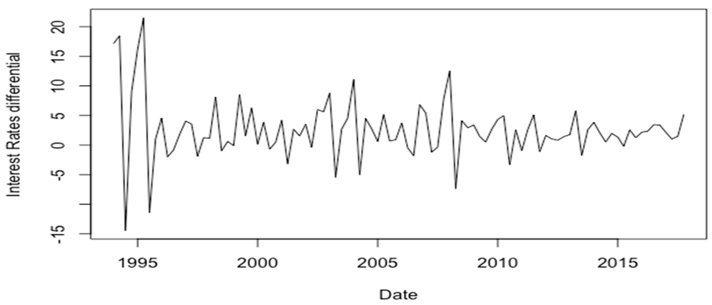
3.3. Interest Rates
3.4. Exchange Rates
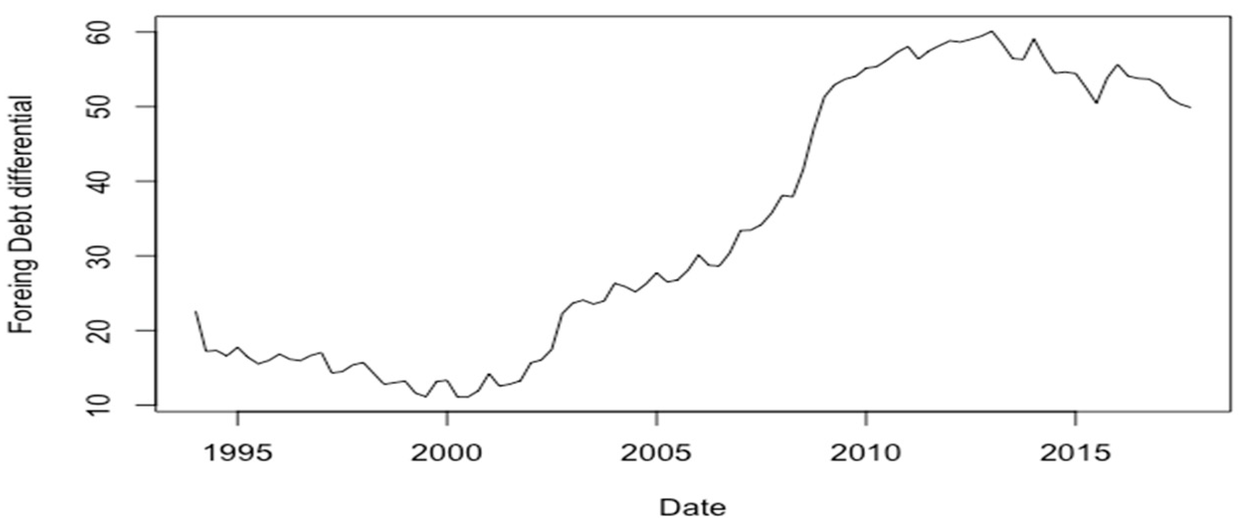
3.5. Domestic Debt
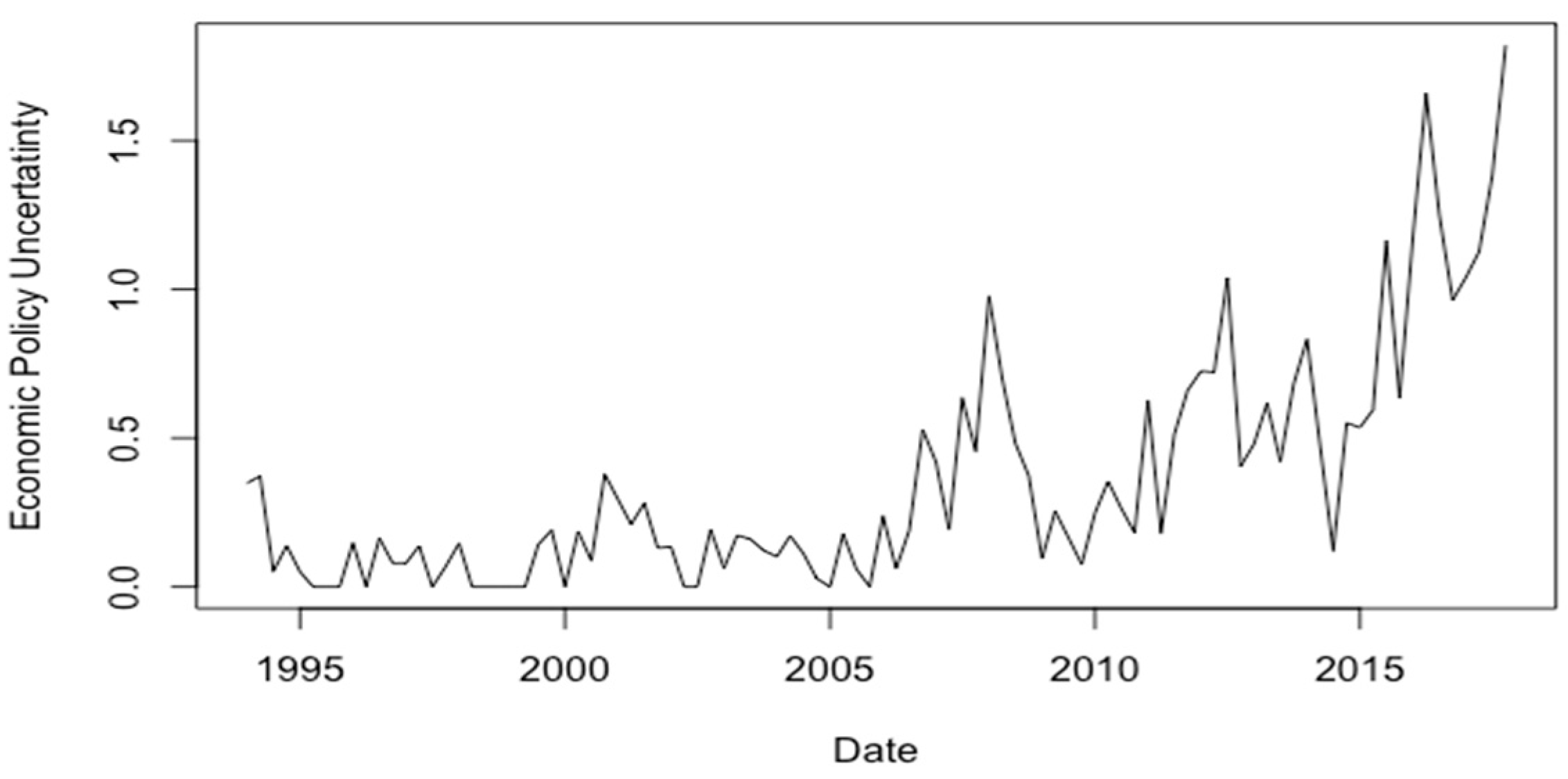
4. Economic Policy Uncertainty
5. Results
6. Conclusions
Author Contributions
Funding
Informed Consent Statement
Data Availability Statement
Acknowledgments
Conflicts of Interest
References
- Almeida, Alvaro, Charles Goodhart, and Richard Payne. 1998. The effects of macroeconomic news on high frequency exchange rate behavior. Journal of Financial and Quantitative Analysis 33: 383–408. [Google Scholar] [CrossRef]
- Armah, Mark Kojo, Isaac Kwesi Ofori, and Francis Kwaw Andoh. 2023. A re-examination of the exchange rate–Interest rate differential relationship in Ghana. Heliyon 9: e14605. [Google Scholar] [CrossRef] [PubMed]
- Auboin, Marc, and Michele Ruta. 2013. The relationship between exchange rates and international trade: A literature review. World Trade Review 3: 577–605. [Google Scholar] [CrossRef]
- Bacchetta, Philippe, and Eric van Wincoop. 2013. On the unstable relationship between exchange rates and macroeconomic fundamentals. Journal of International Economics 91: 18–26. [Google Scholar] [CrossRef]
- Bahmani-Oskooee, Mohsen, and Augustine C. Arize. 2020. On the asymmetric effects of exchange rate volatility on trade flows: Evidence from Africa. Emerging Markets Finance and Trade 4: 913–39. [Google Scholar] [CrossRef]
- Bahmani-Oskooee, Mohsen, and Sahar Bahmani. 2015. Nonlinear ARDL approach and the demand for money in Iran. Economics Bulletin 35: 381–91. [Google Scholar]
- Barbosa-Filho, Nelson H. 2014. Resultado primário, dívida líquida e dívida bruta: Um modelo contábil, em: Bonelli, R. e Veloso, F. (org), Ensaios IBRE de Economia Brasileira II. Rio de Janeiro: Elsevier. [Google Scholar]
- Beckmann, Joscha, Ansgar Belke, and Frauke Dobnik. 2012. Cross-section dependence and the monetary exchange rate model—A panel analysis. The North American Journal of Economics and Finance 23: 38–53. [Google Scholar] [CrossRef]
- Benigno, Gianluca, Pierpaolo Benigno, and Salvatore Nisticò. 2012. Risk, monetary policy, and the exchange rate. NBER Macroeconomics Annual 26: 247–309. [Google Scholar] [CrossRef]
- Ben-Omrane, Walid, Robert Welch, and Xinyao Zhou. 2020. The dynamic effect of macroeconomic news on the euro/US dollar exchange rate. Journal of Forecasting 39: 84–103. [Google Scholar] [CrossRef]
- Bilson, John F. O. 1978. Rational Expectations and the Exchange Rate. In The Economics of Exchange Rates (Collected Works of Harry Johnson): Selected Studies. Abingdon: Routledge, p. 75. [Google Scholar]
- Bjørnland, Hilde C. 2008. Monetary policy and exchange rate interactions in a small open economy. Scandinavian Journal of Economics 110: 197–221. [Google Scholar] [CrossRef]
- Bjørnland, Hilde C. 2009. Monetary policy and exchange rate overshooting: Dornbusch was right after all. Journal of International Economics 79: 64–77. [Google Scholar] [CrossRef]
- Boudt, Kris, Christopher J. Neely, Piet Sercu, and Marjan Wauters. 2019. The response of multinationals’ foreign exchange rate exposure to macroeconomic news. Journal of International Money and Finance 94: 32–47. [Google Scholar] [CrossRef]
- Bouraoui, Taoufik, and Archavin Phisuthtiwatcharavong. 2015. On the determinants of the THB/USD exchange rate. Procedia Economics and Finance 30: 137–45. [Google Scholar] [CrossRef]
- Brink, S., and R. Koekemoer. 2000. The economics of exchange rates: A South African model. South African Journal of Economic and Management Sciences 3: 19–51. [Google Scholar] [CrossRef]
- Caporale, Guglielmo Maria, Fabio Spagnolo, and Nicola Spagnolo. 2018. Exchange rates and macro news in emerging markets. Research in International Business and Finance 46: 516–27. [Google Scholar] [CrossRef]
- Chahrour, Ryan, Vito Cormun, Pierre De Leo, Pablo A. Guerrón-Quintana, and Rosen Valchev. 2021. Exchange Rate Disconnect Redux. Newton: Boston College. [Google Scholar]
- Chen, Cathy W. S., Mike K. P. So, and Richard H. Gerlach. 2005. Assessing and testing for threshold nonlinearity in stock returns. Australian & New Zealand Journal of Statistics 47: 473–88. [Google Scholar]
- Chen, Liming, Ziqing Du, and Zhihao Hu. 2020. Impact of economic policy uncertainty on exchange rate volatility of China. Finance Research Letters 32: 101266. [Google Scholar] [CrossRef]
- Cheung, Yin-Wong, Rasmus Fatum, and Yohei Yamamoto. 2019. The exchange rate effects of macro news after the global financial crisis. Journal of International Money and Finance 95: 424–43. [Google Scholar] [CrossRef]
- Chinn, Menzie David. 1991. Some linear and nonlinear thoughts on exchange rates. Journal of International Money and Finance 10: 214–30. [Google Scholar] [CrossRef]
- Chinn, Menzie David. 1999. A monetary model of the South African Rand. African Finance Journal 1: 69–91. [Google Scholar]
- Clarida, Richard, and Jordi Gali. 1994. Sources of real exchange-rate fluctuations: How important are nominal shocks? In Carnegie-Rochester Conference Series on Public Policy. Amsterdam: Elsevier, December, vol. 41, pp. 1–56. [Google Scholar]
- Corsetti, Giancarlo, Luca Dedola, and Sylvain Leduc. 2018. Exchange Rate Misalignment, Capital Flows, and Optimal Monetary Policy Trade-Offs. Ottawa: Bank of Canada. [Google Scholar]
- Cover, James P., and Sushanta K. Mallick. 2012. Identifying sources of macroeconomic and exchange rate fluctuations in the UK. Journal of International Money and Finance 31: 1627–48. [Google Scholar] [CrossRef]
- Cushman, David O. 2000. The failure of the monetary exchange rate model for the Canadian—US dollar. Canadian Journal of Economics/Revue canadienne d’économique 33: 591–603. [Google Scholar] [CrossRef]
- Cushman, David O. 2008. Real exchange rates may have nonlinear trends. International Journal of Finance & Economics 13: 158–73. [Google Scholar]
- de Bruyn, Riané, Rangan Gupta, and Renee Van Eyden. 2015. Can we beat the random-walk model for the south african rand–us dollar and south african rand–uk pound exchange rates? evidence from dynamic model averaging. Emerging Markets Finance and Trade 51: 502–24. [Google Scholar] [CrossRef]
- Devereux, Michael B., Charles Engel, and Steve Pak Yeung Wu. 2023. Collateral Advantage: Exchange Rates, Capital Flows and Global Cycles (No. w31164). Cambridge: National Bureau of Economic Research. [Google Scholar]
- Dimitriou, Dimitrios, and Dimitris Kenourgios. 2013. Financial crises and dynamic linkages among international currencies. Journal of International Financial Markets, Institutions and Money 26: 319–32. [Google Scholar] [CrossRef]
- Dornbusch, Rudiger. 1976. Expectations and exchange rate dynamics. Journal of Political Economy 84: 1161–76. [Google Scholar] [CrossRef]
- Dube, Smile. 2008. Stock prices and the exchange rate in a monetary model: A ARDL Bounds testing approach using South African data. African Finance Journal 10: 1–27. [Google Scholar]
- Eichenbaum, Martin, and Charles L. Evans. 1995. Some empirical evidence on the effects of shocks to monetary policy on exchange rates. The Quarterly Journal of Economics 110: 975–1009. [Google Scholar] [CrossRef]
- Ellwanger, Reinhard, and Stephen Snudden. 2023. Forecasts of the real price of oil revisited: Do they beat the random walk? Journal of Banking & Finance 154: 106962. [Google Scholar]
- Enders, Walter, and Pierre L. Siklos. 2001. Cointegration and threshold adjustment. Journal of Business & Economic Statistics 19: 166–76. [Google Scholar]
- Engel, Charles. 2016. Exchange rates, interest rates, and the risk premium. American Economic Review 106: 436–74. [Google Scholar] [CrossRef]
- Engel, Charles, and Kenneth D. West. 2005. Exchange rates and fundamentals. Journal of Political Economy 113: 485–517. [Google Scholar] [CrossRef]
- Farhi, Emmanuel, and Xavier Gabaix. 2016. Rare disasters and exchange rates. The Quarterly Journal of Economics 131: 1–52. [Google Scholar] [CrossRef]
- Faust, Jon, and John H. Rogers. 2003. Monetary policy’s role in exchange rate behavior. Journal of Monetary Economics 50: 1403–24. [Google Scholar] [CrossRef]
- Frenkel, Jacob A. 1976. A monetary approach to the exchange rate: Doctrinal aspects and empirical evidence. Scandinavian Journal of Economics 78: 200–24. [Google Scholar] [CrossRef]
- Gau, Yin-Feng, and Zhen-Xing Wu. 2017. Macroeconomic announcements and price discovery in the foreign exchange market. Journal of International Money and Finance 79: 232–54. [Google Scholar] [CrossRef]
- Ghosh, Taniya, and Soumya Bhadury. 2018. Money’s causal role in exchange rate: Do divisia monetary aggregates explain more? International Review of Economics & Finance 57: 402–17. [Google Scholar]
- Gürkaynak, Refet S., A. Hakan Kara, Burçin Kısacıkoğlu, and Sang Seok Lee. 2021. Monetary policy surprises and exchange rate behavior. Journal of International Economics 130: 103443. [Google Scholar] [CrossRef]
- Ha, Jongrim, M. Marc Stocker, and Hakan Yilmazkuday. 2020. Inflation and exchange rate pass-through. Journal of International Money and Finance 105: 102187. [Google Scholar] [CrossRef]
- Hacker Scott, R., Karlsson Hyunjoo Kim, and Månsson Kristofer. 2012. The relationship between exchange rates and interest rate differentials: A wavelet approach. The World Economy 9: 1162–1185. [Google Scholar] [CrossRef]
- Hadebe, Ntokozo, and Simiso Msomi. 2023. Focusing on the Exchange Rate Volatility and International Trade Relationship: Evidence from South Africa. Journal of Management and Economics 8: 354–67. [Google Scholar] [CrossRef]
- Hassan, Shakill, and Félix Simione. 2013. Exchange rate determination under monetary policy rules in a financially underdeveloped economy: A simple model and application to Mozambique. Journal of International Development 25: 502–19. [Google Scholar] [CrossRef]
- Heider, Florian, Farzad Saidi, and Glenn Schepens. 2021. Banks and negative interest rates. Annual Review of Financial Economics 13: 201–18. [Google Scholar] [CrossRef]
- Hina, Hafsa, and Abdul Qayyum. 2015. Re-estimation of Keynesian model by considering critical events and multiple cointegrating vectors. The Pakistan Development Review, 123–45. [Google Scholar]
- Ibhagui, Oyakhilome Wallace. 2019. Monetary model of exchange rate determination under floating and non-floating regimes. China Finance Review International 9: 254–83. [Google Scholar] [CrossRef]
- Inoue, Atsushi, and Barbara Rossi. 2019. The effects of conventional and unconventional monetary policy on exchange rates. Journal of International Economics 118: 419–47. [Google Scholar] [CrossRef]
- Ismailov, Adilzhan, and Barbara Rossi. 2018. Uncertainty and deviations from uncovered interest rate parity. Journal of International Money and Finance 88: 242–59. [Google Scholar] [CrossRef]
- Itskhoki, Oleg, and Dmitry Mukhin. 2021. Exchange rate disconnect in general equilibrium. Journal of Political Economy 129: 2183–32. [Google Scholar] [CrossRef]
- Jabeen, Munazza, and Abdul Rashid. 2022. Macroeconomic News and Exchange Rates: Exploring the Role of Order Flow. Global Journal of Emerging Market Economies 14: 222–45. [Google Scholar] [CrossRef]
- Karahan, Özcan. 2020. Influence of exchange rate on the economic growth in the Turkish economy. Financial Assets and Investing 1: 21–34. [Google Scholar] [CrossRef]
- Kim, Soyoung, and Kuntae Lim. 2018. Effects of monetary policy shocks on exchange rate in small open Economies. Journal of Macroeconomics 56: 324–39. [Google Scholar] [CrossRef]
- Klein, Michael W., and Jay C. Shambaugh. 2015. Rounding the corners of the policy trilemma: Sources of monetary policy autonomy. American Economic Journal: Macroeconomics 7: 33–66. [Google Scholar] [CrossRef]
- Lilley, Andrew, Matteo Maggiori, Brent Neiman, and Jesse Schreger. 2022. Exchange rate reconnect. Review of Economics and Statistics 104: 845–55. [Google Scholar] [CrossRef]
- Ludi, Kirsten L., and Marc Ground. 2006. Investigating the Bank Lending Channel in South Africa: A VAR Approach. Pretoria: University of Pretoria. [Google Scholar]
- Magud, Nicolas E., Carmen M. Reinhart, and Esteban R. Vesperoni. 2014. Capital inflows, exchange rate flexibility and credit booms. Review of Development Economics 18: 415–30. [Google Scholar] [CrossRef]
- Mahmood, Haider, and Tarek Tawfik Yousef Alkhateeb. 2018. Asymmetrical effects of real exchange rate on the money demand in Saudi Arabia: A non-linear ARDL approach. PLoS ONE 13: e0207598. [Google Scholar] [CrossRef] [PubMed]
- Majumder, Amita, and Ranjan Ray. 2020. National and subnational purchasing power parity: A review. Decision 47: 103–24. [Google Scholar] [CrossRef]
- Mallick, Lingaraj, Behera Smruti Ranjan, and Mita Bhattacharya. 2024. Impact of Exchange Rate on Trade Balance of India: Evidence from Threshold Cointegration with Asymmetric Error Correction Approach. Foreign Trade Review 59: 279–308. [Google Scholar] [CrossRef]
- Meese, Richard A., and Kenneth Rogoff. 1983. Empirical exchange rate models of the seventies: Do they fit out of sample? Journal of International Economics 14: 3–24. [Google Scholar] [CrossRef]
- Msomi, S., and H. Ngalawa. 2024. Exchange rate expectations and exchange rate behaviour in the South African context. Studies in Economics and Econometrics 48: 1–17. [Google Scholar] [CrossRef]
- Neely, Christopher J., and S. Rubun Dey. 2010. A survey of announcement effects on foreign exchange returns. Federal Reserve Bank of St. Louis Review 92: 417–63. [Google Scholar] [CrossRef]
- Nell, Kevin S. 2003. The stability of M3 money demand and monetary growth targets: The case of South Africa. Journal of Development Studies 39: 155–80. [Google Scholar] [CrossRef]
- Officer, Lawrence H. 2007. Between the Dollar-Sterling Gold Points: Exchange Rates, Parity and Market Behavior. Cambridge: Cambridge University Press. [Google Scholar]
- Özmen, M. Utku, and Erdal Yılmaz. 2017. Co-movement of exchange rates with interest rate differential, risk premium and FED policy in “fragile economies”. Emerging Markets Review 33: 173–88. [Google Scholar] [CrossRef]
- Pham, Van Anh. 2019. Impacts of the monetary policy on the exchange rate: Case study of Vietnam. Journal of Asian Business and Economic Studies 26: 220–37. [Google Scholar] [CrossRef]
- Rapach, David E., and Mark E. Wohar. 2006. The out-of-sample forecasting performance of nonlinear models of real exchange rate behavior. International Journal of Forecasting 2: 341–61. [Google Scholar] [CrossRef]
- Rastogi, Shailesh, Adesh Doifode, Jagjeevan Kanoujiya, and Satyendra Pratap Singh. 2023. Volatility integration of gold and crude oil prices with the interest rates in India. South Asian Journal of Business Studies 12: 444–61. [Google Scholar] [CrossRef]
- Raza, Syed Ali, and Sahar Afshan. 2017. Determinants of exchange rate in Pakistan: Revisited with structural break testing. Global Business Review 18: 825–48. [Google Scholar] [CrossRef]
- Rehman, Muhammad Ateeq, Syed Ghulam Meran Shah, Lucian-Ionel Cioca, and Alin Artene. 2021. Accentuating the Impacts of Political News on the Stock Price, Working Capital and Performance: An Empirical Review of Emerging Economy. Rom. J. Econ. Forecast 2: 55–73. [Google Scholar]
- Saeed, Ahmed, Rehmat Ullah Awan, Maqbool H. Sial, and Falak Sher. 2012. An econometric analysis of determinants of exchange rate in Pakistan. International Journal of Business and Social Science 3: 184–96. [Google Scholar]
- Sichei, Moses Muse, Tewodros G. Gebreselasie, and Olusegun Ayodele Akanbi. 2005. An Econometric Model of Rand-US Dollar Nominal Exchange Rate. Pretoria: University of Pretoria. [Google Scholar]
- Smales, Lee A. 2022. The influence of policy uncertainty on exchange rate forecasting. Journal of Forecasting 41: 997–1016. [Google Scholar] [CrossRef]
- Soon, Siew-Voon, and Ahmad Zubaidi Baharumshah. 2021. Exchange rates and fundamentals: Further evidence based on asymmetric causality test. International Economics 165: 67–84. [Google Scholar] [CrossRef]
- Tari, Recep, and Mehmet Çağrı Gözen. 2018. Portfolio balance approach to exchange rate determination: Testing a model by applying bilateral data of Turkey and United States 1. Ege Akademik Bakis 18: 423–34. [Google Scholar]
- Tawadros, George B. 2017. Revisiting the exchange rate disconnect puzzle. Applied Economics 49: 3645–68. [Google Scholar] [CrossRef]
- Tong, Howell. 1983. Threshold Models in Non-Linear Time-Series Analysis. Lecture Notes in Statistics 21. New York: Springer. [Google Scholar]
- Valchev, Rosen. 2020. Bond convenience yields and exchange rate dynamics. American Economic Journal: Macroeconomics 12: 124–66. [Google Scholar] [CrossRef]
- Xie, Zixiong, and Shyh-Wei Chen. 2019. Exchange rates and fundamentals: A bootstrap panel data analysis. Economic Modelling 78: 209–24. [Google Scholar] [CrossRef]
- Zettelmeyer, Jeromin. 2004. The Impact of Monetary Policy on the Exchange Rate: Evidence from Three Small Open Economies. Journal of Monetary Economics 51: 635–52. [Google Scholar] [CrossRef]
- Ziramba, Emmanuel. 2007. Measuring exchange market pressure in South Africa: An application of the Girton-Roper monetary model: Economics. South African Journal of Economic and Management Sciences 10: 89–98. [Google Scholar] [CrossRef]


| Variable | Coefficient |
|---|---|
| Debt differential | 2.421309 *** |
| Economic policy uncertainty | −0.259494 * |
| Interest rate differential | −0.029141 * |
| Lower threshold value 0.6827 | |
| Debt differential | 0.297169 |
| Economic policy uncertainty | −4.259460 *** |
| Interest rate differential | −0.065262 |
| Upper threshold value = 0.8655 | |
| Debt differential | 0.473598 *** |
| Economic policy uncertainty | 0.541118 ** |
| Interest rate differential | 0.133507 * |
Disclaimer/Publisher’s Note: The statements, opinions and data contained in all publications are solely those of the individual author(s) and contributor(s) and not of MDPI and/or the editor(s). MDPI and/or the editor(s) disclaim responsibility for any injury to people or property resulting from any ideas, methods, instructions or products referred to in the content. |
© 2024 by the authors. Licensee MDPI, Basel, Switzerland. This article is an open access article distributed under the terms and conditions of the Creative Commons Attribution (CC BY) license (https://creativecommons.org/licenses/by/4.0/).
Share and Cite
Msomi, S.; Ngalawa, H. The Monetary Model of Exchange Rate Determination for South Africa. Economies 2024, 12, 206. https://doi.org/10.3390/economies12080206
Msomi S, Ngalawa H. The Monetary Model of Exchange Rate Determination for South Africa. Economies. 2024; 12(8):206. https://doi.org/10.3390/economies12080206
Chicago/Turabian StyleMsomi, Simiso, and Harold Ngalawa. 2024. "The Monetary Model of Exchange Rate Determination for South Africa" Economies 12, no. 8: 206. https://doi.org/10.3390/economies12080206
APA StyleMsomi, S., & Ngalawa, H. (2024). The Monetary Model of Exchange Rate Determination for South Africa. Economies, 12(8), 206. https://doi.org/10.3390/economies12080206