Public R&D and Growth: A dynamic Panel Vector-Error-Correction Model Analysis for 14 OECD Countries

Abstract

This paper addresses the controversial issue of the direct and indirect effects of public R&D on growth. We look at six variables of R&D-driven growth jointly for 14 OECD countries using methods of dynamic systems for panel data analysis: GDP, technical change, domestic and foreign businesses and public R&D. Cointegration tests suggest four long-run relations for the six variables. We estimate these relations using group mean versions of fully modified and dynamic OLS. Domestic public R&D has positive long-run regression coefficients for direct effects on productivity and indirect ones via private R&D. Here, we build a panel vector-error-correction model with these long-term relations. Shocks to domestic public R&D enhance domestic private R&D, technical change and the GDP. Permanent changes in foreign public and private R&D have positive growth effects, which are transitional for foreign public R&D.

1. Introduction

GDP growth per capita is driven mainly by technical change and human and physical capital (see Appendix A). Development economics adds effects mostly related to capital accumulation and labor growth (Perkins et al. 2013). Endogenous growth theory mainly models technical change that is driven by private research and development (R&D) (Helpman 1992). Lucas (2015) suggests that technical change is effectively identical to human capital. This paper is in line with others discussed below, seeing technical change as driven by private and public R&D, where the expenditures include those for human capital.

Although private R&D is widely accepted as a driving force, the role of public R&D is more controversial in the empirical literature. Erken et al. (2018) and Herzer (2022) emphasize ‘ambiguous results in the literature’ on public R&D and growth. van Elk et al. (2015, 2019) analyzed the rate of return for public R&D for a panel of OECD countries. While analyzing a Cobb–Douglas function for total factor productivity (TFP) with slope homogeneity (all countries have the same regression coefficient), they found a negative or zero rate of return for public R&D. After moving to a translog function, international control variables and some country-specific slope heterogeneity through interaction effects similar to those of Khan and Luintel (2006), they found more positive results, especially in the augmented production function model, but overall, the authors remain sceptic about the effect of public R&D on TFP and see the value of public R&D in aspects other than TFP. In contrast, Huang et al. (2023) consider one of the positive coefficients for public R&D of van Elk et al. (2015, 2019) as the most convincing result in the literature on public R&D and growth. Erken et al. (2008) found a positive effect of public R&D in a panel of 20 OECD countries. However, their method did not yield a t-value for the coefficient of public R&D because of a specific way of imposing constraints on estimated coefficients. Donselaar and Koopmans (2016) found an output elasticity of public R&D of 0.03 in a meta-analysis for a small set of studies, but it was statistically insignificant.1

On the other hand, there are high rates of return for publicly funded R&D in the USA, as reported by Fieldhouse and Mertens (2023), as well as for publicly performed R&D in studies of Soete et al. (2020, 2022) and for mission oriented R&D in Ziesemer (2021b). These results come from three economically different approaches explained in Section 2.1, Section 2.2 and Section 2.3 and from some econometric choices explained in Section 2.4 and changed in this paper.

In comparison, our approach to showing the positive direct and indirect effects of public R&D on growth is based on six innovations using dynamic system methods for panel data (Hsiao 2022, chp. 5): (i) We establish four long-term relations between R&D variables, productivity and GDP with slope homogeneity using group mean versions of DOLS (Dynamic Ordinary Least Squares) and FMOLS (Fully Modified Ordinary Least Squares) with fixed effects as well as cointegration tests, whereas other panel studies have only one relation. Without cointegration, unit roots may lead to unstable regression coefficients. (ii) We provide a panel VECM (vector-error-correction model) with fixed effects in the differenced part and statistically significant adjustment coefficients also, making the long-term relations feed back into the dynamic simultaneous equation system, whereas other panel studies estimate only one equation. (iii) We use impulse response analysis of shocks on public R&D and foreign R&D in the panel VECM, for which panel studies in the area of innovation have not yet been conducted.2 (iv) We show positive shock effects of public on private R&D in this new panel VECM setting, which have been shown for single countries in other papers. (v) We show the effects of public R&D directly and indirectly on productivity, which, so far, exists only in single-country studies. (vi) We show positive shock effects of foreign public and private R&D shocks on growth, whereas panel studies, so far, have used only aggregated foreign R&D.

Section 2 motivates the purpose of this paper in more detail. The data are described in Section 3 and the econometric methods in Section 4. The major estimation results presented in Section 5 (besides those on unit roots and panel cointegration) are that the direct and indirect long-run effects of public R&D via private R&D on productivity always turn out to be positive when using FMOLS or DOLS estimation methods for the long-term relation, which are the current standard for long-term relations in panel VECMs (Hsiao 2022). The effects of public and foreign R&D are also positive when using shock simulations considering, also, the short-term effects and adjustment processes towards the FMOLS- or DOLS-based cointegrating equations, shown in Section 6. Section 7 summarizes and concludes the article with suggestions for further research.

2. Economic and Econometric Approaches of the Literature to Public R&D Analysis

2.1. Direct Effects of Public R&D in the Traditional Standard Approach

The standard approach used in the literature has a Cobb–Douglas output production function with a TFP variable and a Cobb–Douglas TFP production function depending on R&D stocks (OECD 2017; Hall et al. (2010). Public R&D stocks are put into the TFP equation, and therefore, only the direct effects of public R&D stocks on productivity are considered (although van Elk et al. (2015, 2019) discuss indirect effects verbally, and Herzer (2022) presents them in a theoretical model). Examples in the literature are Guellec and van Pottelsberghe de la Potterie (2004), Erken et al. (2008, 2018), van Elk et al. (2015, 2019), Herzer (2022) for OECD country panels, Pegkas et al. (2020) for a Eurozone panel, Voutsinas and Tsamadias (2014) for Greece, Bengoa et al. (2017) for Spanish regions and Fieldhouse and Mertens (2023) for the USA. OECD (2017) surveys in the literature are mainly on aggregate R&D until 2014.

2.2. Indirect Effects of Public R&D in an Endogenous Growth Approach

In contrast, Park (1998) models TFP only as depending on a private R&D stock variable, A_p, implying that direct effects of public R&D on productivity are excluded by assumption. Formally,

TFP = A_pF(K,H_Y), dA_p = H_pF_p(A_p; A_g), dA_g = H_gF_g(A_p; A_g).

Only A_p enters the output and TFP production function (besides the physical capital K and human capital H_Y) in Park’s study (Park 1998), whereas in the standard model, A_g (public R&D stocks) and the foreign R&D stock(s) would also be included. Standard cost minimization considerations would have the human capital cost qH_p as the R&D expenditure flow, with q as the factor price of human capital demand H_p. Summing the changes dA and expenditure flows over time, A is equal to the R&D expenditure stock; for A_p (A_g), this is only private (public) R&D expenditure. A terms and R&D stock variables are then equal and can replace each other. For A_g, this is public R&D expenditure, which enters the production of dA_p only as an externality, and A_g does not enter the TFP directly like A_p does; similarly, A_p is an externality in the production of dA_g, but it is included in the TFP function. Public R&D goes only into the production of private and public knowledge and, therefore, only indirectly into the TFP. This is motivated by finding a negative (positive) effect of public R&D when (not) controlling for private R&D in Park’s study (Park 1995) in the model without spillovers. We will show positive and statistically significant direct and indirect effects in the long-term relations estimated using DOLS and FMOLS, taking into account endogeneity and nonstationarity (other methods do not do this), which are inserted into the panel VECM. This result is similar to that of Guellec and van Pottelsberghe de la Potterie (2003a, 2004), who found positive direct effects and positive (negative) indirect effects from civilian (defense) R&D via an interaction term with private R&D in an unconstrained single-equation ECM. However, we find this effect without leaning on interaction terms.

2.3. Direct and Indirect Effects of Public R&D in VECMs

Herzer (2022) drops A_p from the third equation of Park’s theoretical model (Park 1998) and also puts H_g into the second function, allowing for direct effects of public R&D flows on productivity in addition to the indirect ones emphasized by Park (1998); these steps lead to the interesting result of a higher elasticity of productivity of public compared to private R&D. In terms of Cobb–Douglas functions, these changes in assumptions raise the question whether certain elasticities of productivity functions are zero or positive. Ziesemer (2021a) raised this question in terms of the generalized CES function of Mukerji (1963), which is log-linear in terms of the first-order conditions of optimum growth or profit maximization.3 Recent country-specific VECMs by Soete et al. (2020, 2022) and Ziesemer (2020, 2021a, 2021b, 2022, 2024a) using log-linear relations with time trends in the long-term relations for 17 OECD countries separately bring direct and indirect effects together. These papers go more deeply into the analysis of slope heterogeneity by way of analyzing one vector-error-correction model (VECM) per country. They go beyond Coe and Helpman (1995) and Luintel and Khan (2004) by splitting domestic and foreign R&D into private (business) and public (non-business) R&D, which Erken et al. (2008) achieve only in a single-equation panel regression; moreover, they have several long-term relations. Soete et al. (2022) found that the most frequent constellation is the stylized result of five relations, suggesting that (i) TFP drives GDP, (ii) private R&D drives TFP, (iii) public R&D drives private R&D, (iv) foreign public R&D drives domestic public R&D and (v) foreign private and foreign public R&D drive each other. Constellations of four or three long-term relations with three or four variables, respectively, are slightly less frequent. In line with van Elk et al. (2015, 2019), Bengoa et al. (2017) and the use of control variables by Erken et al. (2008), they found that national circumstances play a role. Public R&D may have differing direct effects on TFP or indirect ones via private R&D or through the whole system.4 However, the emphasis in VECMs is, in the first instance, not on direct or indirect effects but rather on normalizing three, four or five long-term relationships (obtained from the Johansen trace and maximum eigenvalue tests) in a way that they are economically meaningful and statistically significant. In fact, the issue of re-normalization leads to different versions of the cointegrating equations, but the interpretation of shocks is in line with the five relations indicated here. As a by-product of this normalization and the shock analysis, Soete et al. (2022) found positive (negative) indirect effects of public on private R&D for Austria, Denmark, France, Ireland, Italy, Japan, Norway, the UK and (Belgium) and positive (negative) direct effects for the Netherlands, Norway, Portugal, Spain, (Belgium, Denmark and Ireland). The VECM does take into account interactions between all the variables mentioned and not only those allowed for in Park’s model (Park 1998) or restrictive modifications of it. The total effect from analysis of shocks (impulse response) on public R&D are positive for all countries except for Canada, France and Ireland. For some other countries, the rate of return for public R&D is only positive under the additional condition that the policy of enhancing public R&D is stopped before periods in which the gains become negative. Rates of return differ across countries. An in-depth analysis of the heterogeneity in the country-specific results shows, among other aspects, that the total effects are mostly not positive if the positive indirect effect of public on private R&D does not work in the impulse response analysis for a small number of countries (Soete et al. 2022). However, even if the indirect effect works, the direct effect and the system effect may work against it, as in the case of Ireland. For Canada, Loertscher and Pujolas (2024) attribute 20 years of TFP stagnation to high oil sector inputs; country-specific aspects of inputs may reduce TFP growth and undermine the relevance of R&D interactions for some phases of time. However, our analysis below shows that these are exceptions that are not dominating the panel data analysis in the dynamic systems approach using a VECM.

2.4. Choices in Panel Data Econometrics

Having results per country, there seems to be no econometric need for pooling (Hsiao 2022) other than for having more observations. However, when seeing the extent of heterogeneity found by Soete et al. (2022) (differences in the numbers and normalizations of cointegrating equations, as well as results from shocks and rates of return), at least some readers would like to see something simpler and more structured as under slope homogeneity. One case in point is the desire to find a coefficient value that can be used in the calibration of simulation models (Adema et al. 2023).5 This may generate the desire for pooled data from similar countries. Pooling requires an assumption, which is that countries are sufficiently similar for every regression with slope homogeneity. In this paper, we take Canada, France and Ireland out of the OECD sample because public R&D does not have the expected effect on productivity in Soete et al. (2022). This is an application of the more general rule that in panel data analyses using slope homogeneity, we should not have a set of countries that is too heterogeneous because it may lead to heterogeneity bias or have a non-representative impact in mean-group estimation. Therefore, we perform some panel data analyses for the remaining 14 OECD countries. We use two approaches:

(i)

Cointegration tests show the relation for the pairs of variables mentioned above; three of the five pairs have no panel cointegration, and therefore, we go from five pairs to four triples of variables that do have cointegration6 and are estimated using cointegrating regression methods, FMOLS and DOLS:

• GDP–productivity;
• Productivity–private R&D–public R&D;
• Private R&D–public R&D–foreign private R&D;
• Public R&D–foreign private R&D–foreign public R&D.

(ii)

We use a vector-error-correction model with these four cointegrating equations from group mean versions of DOLS and FMOLS estimations with cross-section fixed effects and, in the differenced part, fixed effects and slope homogeneity in the regression coefficients and the adjustment coefficients. This a restricted version of the panel VECM suggested in the econometric literature (Hsiao 2022, chp. 5.3.2.1). It allows us to run simulations of shock effects going through all six equations for growth of the endogenous GDP, productivity and four R&D variables mentioned above (see Section 4).7 We find positive direct and indirect effects of public R&D on productivity in the long-term relations obtained via DOLS and FMOLS and also through the shocks on the public R&D equation.

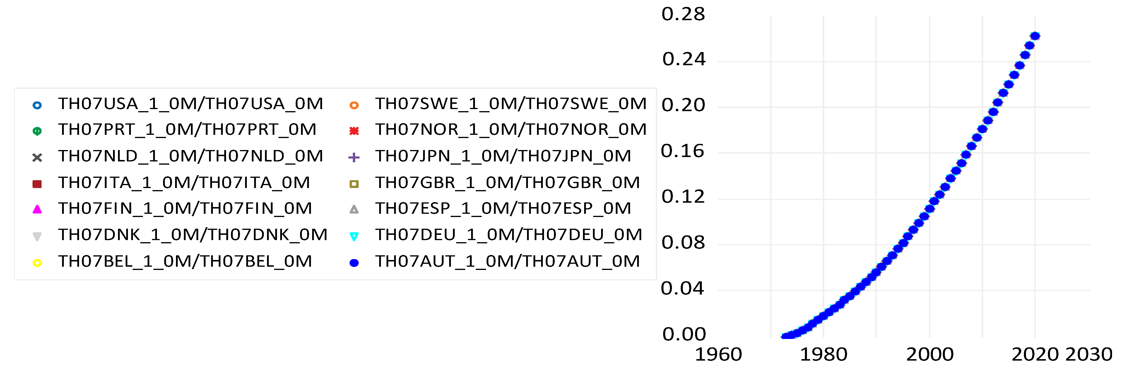
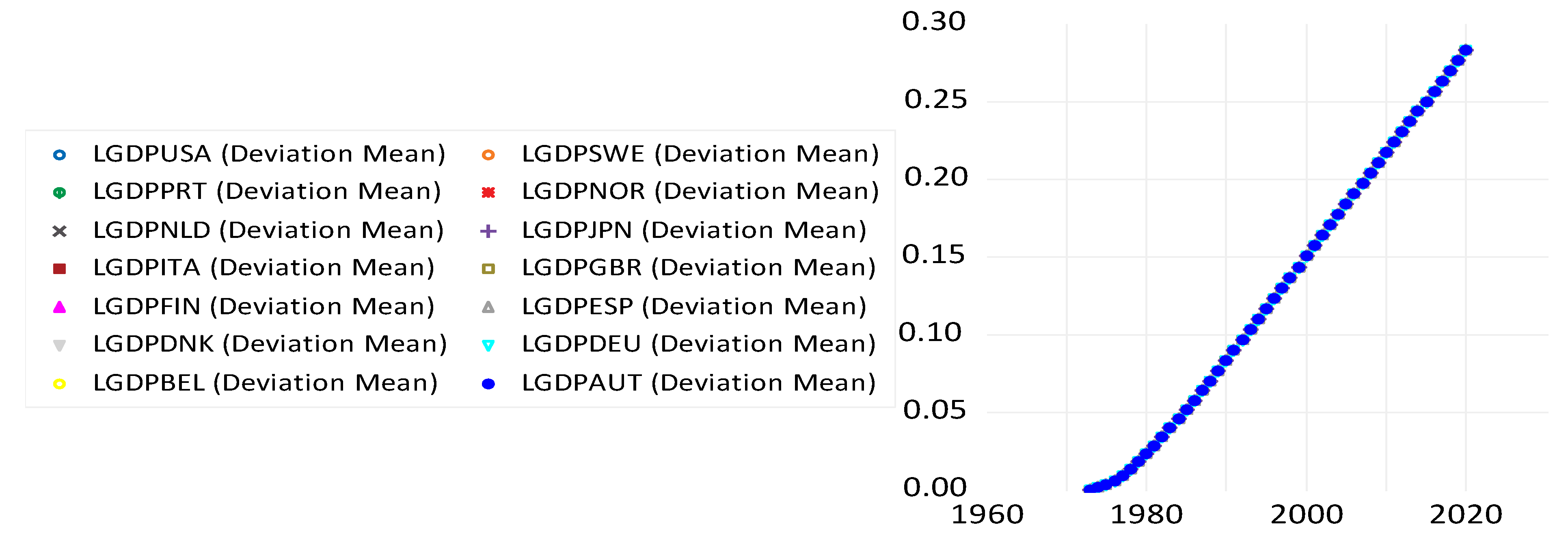
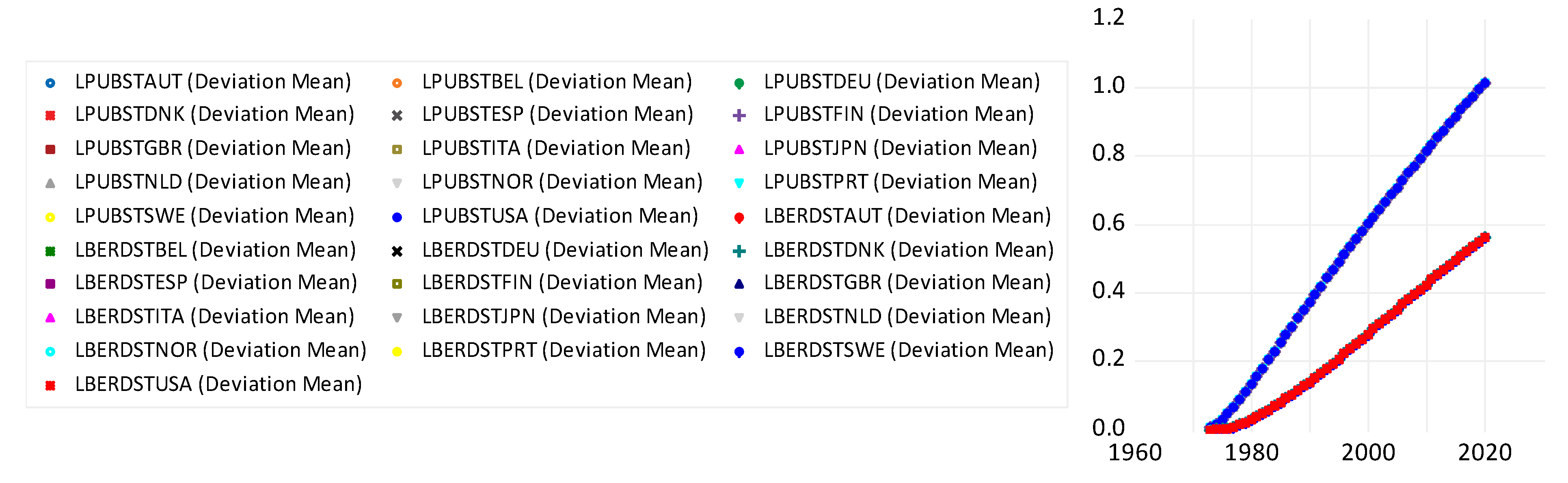
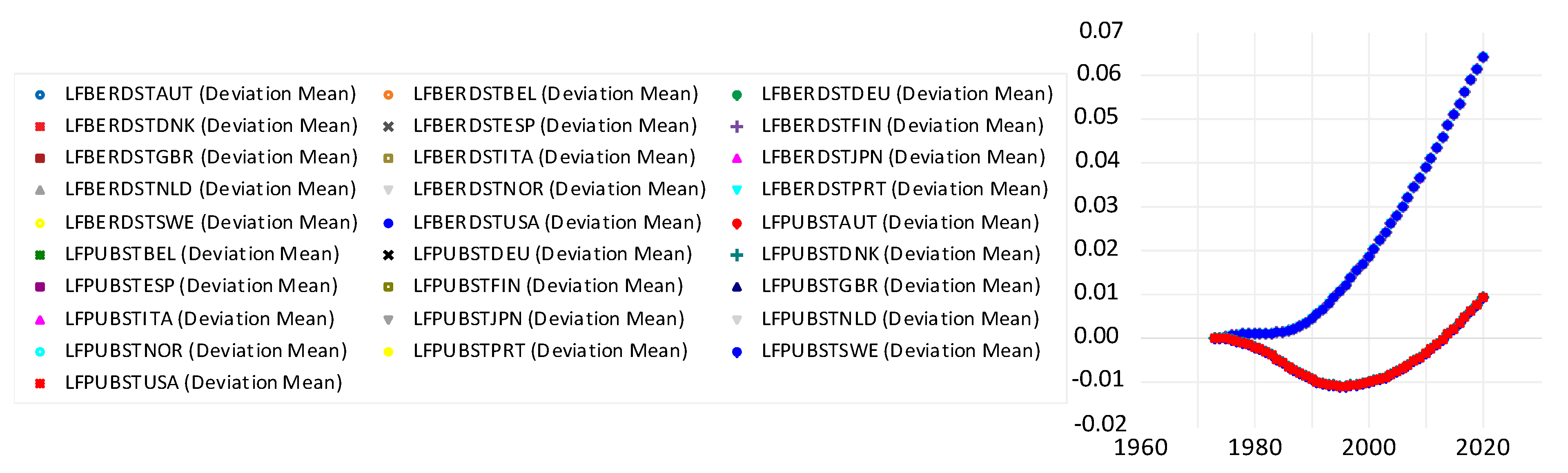
The combination of these approaches in a VECM has three advantages in comparison to the standard procedure.8

First, we do not impose having only one (cointegrating) equation for productivity, which would press all information for five or four relations into one equation; instead, we assume, after testing for cointegration, four triple-wise cointegrated relations, which generate more and better information (Kilian and Lütkepohl 2017, p. 103) that is typically shown through a higher log-likelihood for models with more cointegrating relations, provided they are economically plausible and statistically significant. This allows us to deal explicitly with the suggestions of Park (1995) and Sveikauskas (2007), theoretically modeled by Park (1998), that public R&D works mainly through its effect on private R&D and, therefore, only indirectly on productivity.9 Comparisons with the extended standard model, modeling only the direct effects of public R&D on productivity, and the extended Romer model of Park (1998), modeling only the indirect effects via private R&D on productivity, suggests that the standard model has tested only for the direct effects but not for the indirect effects of public R&D stocks working via the private R&D stock.10 The methods used in this paper test for both effects. Similarly, foreign private R&D may have a direct effect on domestic business R&D in line with oligopoly theory (see Ziesemer 2022) and an indirect one via its effect on domestic public R&D. For the role of foreign R&D too, Park (1998) models only the indirect effects, and van Elk et al. (2015, 2019) as well as Pegkas et al. (2020) model only the direct effects on TFP.11 Having several long-term relations allows us to treat the controversial effects of public and foreign R&D differently than investigations using only one long-term relation.

Second, cointegrating equations with a log–log specification do not necessarily use Cobb–Douglas or translog functions but may be more closely related to the first-order conditions based on the SMAC VES (variable elasticity of substitution) of Mukerji (1963),12 which generalizes the CES function by way of giving the CES parameter an index of the related argument (see Ziesemer 2021a).13

Third, the use of a VECM allows us to apply shock or impulse response analysis to the solution of the panel data VEC model and test whether good-looking partial regression results also lead to plausible, similar outcomes under a shock on public R&D growth and related variables in a multi-equation system.14

We tend to speculate that these three methodological issues, which we discuss at the proper time, are behind ‘ambiguous results in the literature’ (Erken et al. 2018; Herzer 2022) on public R&D (besides slope heterogeneity and missing time trends)15. They belong to the modern time-series and panel time-series methods, which are made possible by the availability of longer data series compared to the databases in the literature surveyed in the OECD (2017).

3. Data

We use data from 14 OECD countries for which we have relatively long data series.16

The data are an updated version of those in the studies of van Elk et al. (2015, 2019) and Soete et al. (2022), using recent updates of the sources that extend the time period from 1963 to 2017. More recent years in the OECD MSTI (main science and technology indicators) end in 2021 and have gaps even for our 14 countries or are characterized as provisional or estimated. Articles using data for more countries have series starting later (see Herzer (2022) for a detailed listing). There are also countries where the data have many gaps. We use only data for countries with long series and limited missing data points, as indicated in

Table 1. Data information for 14 OECD countries (1963–2017).

Variable	Mean	Median	Stdev	Min	Max	Growth Rate (a)	P (No csd) (b)	Data Points, obs (c)
LGDP	13.12	12.71	1.137	10.7	16.6	0.0166 + 0.35g(−1)	0.0000	770; 742
LTH07	1.888	1.906	0.336	0.66	2.80	0.0124 + 0.144g(−1)	0.0000	770; 742
LBERDST	10.1	10.0	1.86	5.76	14.4	0.0055 + 0.8g(−1)	0.0000	749; 721
LPUBST	9.780	9.469	1.526	6.62	13.5	0.0042 + 0.872g(−1)	0.0000	744; 716
LFPUBST	12.7	12.79	0.702	10.2	13.7	0.0039 + 0.849g(−1)	0.0000	770; 742
LFBERDST	13.28	13.38	0.785	10.7	14.4	0.00315 + 0.898g(−1)	0.0000	770; 742

(a) From panel LS regression of g (log difference) on g(−1) and constant with country and period fixed effects. (b) p values for four standard tests (Breusch–Pagan LM, Pesaran scaled LM, bias-corrected scaled LM, Pesaran CD) are all 0.0000 for null ‘no cross-section dependence’ for the variable in the pre-column. (c) Compared to 14 × 55 = 770 data points under full availability; the difference equation loses observations because of lags and taking growth rates.

.

The GDP is from the Penn World Tables (version 9.1; Feenstra et al. 2015). We use the national accounts version for the GDP (RGDPNA in PWT terminology). PWT 10 or 10.01 would go to 2019, but given the limit with OECD MSTI ending 2021, this would only allow two additional years.

For technical change, we use the data from Ziesemer (2023a) for labor-augmented technical change derived from a CES function (including human capital explicitly in the CES function and, by implication, not in the technical change measure) under the assumption of an elasticity of substitution of 0.7 denoted as TH07, and these are based on PWT data. TFP data from the PWT are not used because they are based on controversial capital stock data (Inklaar et al. 2019) and on the assumption of Cobb–Douglas production functions implying an elasticity of substitution of unity, which is sometimes unrealistic. Ziesemer (2023a) avoids both pitfalls and explains this in detail.

R&D flow data come from the OECD MSTI, and, as in the cases of van Elk et al. (2019) and Soete et al. (2022), we use older versions of the OECD database kept at UNU-MERIT to extend the coverage of R&D data back to the 1960s. Gaps in the R&D data are filled by interpolating the R&D intensity (R&D as a share of GDP) and using GDP data to recover the implied R&D expenditures. The time series for R&D expenditures are then converted into R&D capital stocks to represent the idea that it is not only current R&D expenditures that influence productivity but rather the accumulated knowledge that results from present and past R&D expenditures. It is also assumed that this accumulated knowledge depreciates; we use a rate of 15%, as in the literature (Hall et al. 2010).17 We use a perpetual inventory method to construct the stocks: St = (1 − 0.15)St − 1 + Rt, where S is the stock, and R is the current expenditure. We apply this to both public and private R&D, yielding a stock for both types of R&D, abbreviated as BERDST and PUBST. Private R&D expenditures are expenditures for R&D performed by business enterprises, and public R&D expenditures are total domestic expenditures minus business enterprise expenditures (Higher Education and public labs are the largest categories of public expenditures defined in this way).18 For details of constructing initial values, ‘We also need to assume a value for the growth rate of the stock for the initial period. This is chosen to minimize the difference between the initial growth rate and the next one that results from the formula.’ (Soete et al. 2022).

An L in the beginning of the variable name indicates the natural logarithm. An F indicates ‘foreign’. ‘Foreign’ variables are obtained by adding the R&D flows from 16 OECD countries (Canada, France and Ireland can, of course, also generate spillovers to the 14 countries included in our panel analysis) weighted by distance and then following, again, the aggregation procedure indicated above. In the trade literature, FDI and migration have been suggested as weights. They are all controversial and linked to distance, which, therefore, seems plausible (Luintel and Khan 2004; van Elk et al. 2015, 2019). Linking foreign R&D variables to domestic R&D variables is a way to take into account cross-unit cointegration, because not all variables are from the domestic economy. Table 1 indicates the basic numbers of the variables in the form used in the regressions. The third but last column indicates that growth rates are a fraction of their previous value plus a constant and will converge asymptotically to a constant growth rate. The second but last column indicates that the single series have cross-section dependence according to all four standard tests, all with p = 0.0000 for the null hypothesis of ‘no cross-section dependence’.

4. Econometric Methods

4.1. Unit Roots in the Presence of Cross-Section Dependence

Panel unit root tests for any variable y with change ∆y, country index i and period index t in the presence of cross-section dependence are based on the following equation with time trend t and number of lags p (Pesaran 2007; Baltagi 2021; Hsiao 2022):

$${∆y}_{i,t}={\alpha }_i+{\delta }_{i}t+{\gamma }_i{y}_{i,t-1}+\sum _{l=1}^{p_i}{\phi }_{il}{∆y}_{i,t-l}+c_i{\overline{y}}_{t-1}+\sum _{l=0}^{p_i}{d}_{il}{\overline{∆y}}_{t-l}+u_{it}$$

(1)

The first four terms on the right-hand side are known as the Dickey–Fuller equation for unit root tests. Because of the cross-section dependence (csd) of the residuals, Pesaran (2007) adds a common factor f_t assumed to cause the cross-section dependence to the first four terms. Averaging over the left-hand and right-hand sides of (1) allows for solving f_t in the form of the last two terms of (1), which are cross-section averages and can be used in the empirical work to take cross-section dependence into account (see also Smith and Fuertes 2016). This is a special case of only one common factor where the unit root test is ${\gamma }_i=0$ in (1), which would lead to having (1) in differenced terms only. The test is called the CIPS (cross-sectionally augmented Im–Pesaran–Shin test) and is used for finding panel unit roots in variables but not for the application to residuals in cointegration testing. Bai and Ng (2004) developed a method with more common factors from models of factor analysis, which explicitly addresses unit root testing for residuals as a cointegration test. Bai and Ng (2004) and Ahn and Horenstein (2013) developed different approaches to finding the optimal number of common factors, leaning on the most important principal components or on eigenvalue and growth ratios. We add some simple standard tests ignoring cross-sectional dependence (csd) for comparison to indicate that csd changes the results.

4.2. Cointegration Testing Linked to VECMs and Residual-Based Tests

All variables are likely to have unit roots, which may lead to coefficients that are unstable in regard to slight changes in the regression procedure and, therefore, spurious (Section 5 reports the results) in the absence of cointegration. Unit roots undermine the standard methods of statistical interference,19 so we need to test for the cointegration of the pairs of variables for the five central growth relations. For examples like the five relations presented in the Introduction, note that ‘the test20 may lack the power to detect all cointegration relationships and, as a result, may understate the true cointegrating rank …. Hence, it is recommended to apply cointegration tests to all possible subsystems as well and to verify whether the results are consistent with those for the full model. For example, in a K-dimensional system where all variables are individually I(1) (integrated of order one meaning ‘stationary after differentiating once’), if all variables are cointegrated in pairs, the cointegrating rank must be K − 1. Cointegration for the bivariate subsystems may be easier to analyze than cointegration in the full K-dimensional system. This observation suggests that one should analyze the subsystems first and then assess whether the subsystem results are consistent with the results for the full system, …’ (Kilian and Lütkepohl 2017).21

Following this advice for our panel data set, we should test cointegration for all five relations as pairs of variables. If we do not find five cointegrating relations, r = 5, and we should go to four triples of variables, r = 4, and, again, test for cointegration, proceeding this way until we find cointegration, or, in the end, no cointegrating relation for all six variables together. This order of proceeding is the opposite of that in the trace test and maximum-eigenvalue test (see below). For each country and pair of variables, there could be a vector-error-correction model like in (2), explained, in detail, in Section 4.3.

$${dy}_t=\alpha {\beta }^{\prime }{y_{t-1}+B}_{1}d{y}_{t-1}+B_2{dy}_{t-2}+\cdots B_{p-1}{dy}_{t-\left(p-1\right)}+c{X}^{\prime }+u_t$$

(2)

The number of variables for each pair under consideration here is K = 2, and in the case of rejection of cointegration for one of the pairs, we go to triples, K = 3, and so forth. α is the matrix of adjustment coefficients. β is the matrix of coefficients of the cointegrating equations. α and β are matrices of format (K, r) in the first instance (2, r), implying that ${\beta }^{\prime }$ has the format (r, K) = (r, 2) and $\alpha {\beta }^{\prime }$ has the format (K, K) = (2, 2). ${\beta }^{\prime }{y}_{t-1}=u_{t-1}$, and with the format (r, K), (K, 1) = (r, 1) are the r long-term, cointegrating equations with the expected (equilibrium) value zero. The trace test (and perhaps, in addition, the maximum eigenvalue test) is used to find the number of cointegrating equations or eigenvectors, r, by way of testing whether the corresponding eigenvalues are sufficiently different from zero. If r = 0, there are no eigenvectors and eigenvalues statistically different from zero, and therefore, there is no cointegration, and (2) is estimated in differences. If r = 1, we have one cointegrating equation and one unit eigenvalue. If r = 2, the matrix $\alpha {\beta }^{\prime }$ has full rank, indicating that there are no unit eigenvalues, and the system of two equations can be estimated as a VAR in levels. The p-values for the hypotheses ‘at most 0, 1, or 2 cointegrating equations’ for each country are then used to carry out the Fisher–Johansen test for the panel (Maddala and Wu 1999). The statistic $-2\sum _{i=1}^{N}ln{p}_i$ has a chi-square distribution with 2N degrees of freedom, where N = 14 is the number of countries in our case. Note that ln p_i < 0. For low p_i values for the hypothesis r = 0, the chi-square statistic is high, and the p-value of the chi-square test is low, leading to the rejection of the hypothesis r = 0. The test continues, going to the hypothesis r = 1. If the p_i values for r = 1 are high, the chi-square statistic is low, the p-value for the panel hypothesis is high, and r = 1 is not rejected. If the hypothesis is rejected instead, the result is r = K = 2; there is no unit eigenvalue in the system, and the estimations can be conducted in levels without combining them with differenced terms.

Kao’s (1999) panel cointegration test is also reported. It is residual (Engle–Granger) based, searching for a unit root in the residuals of the regression of interest. It has the null hypothesis ‘no cointegration’. From the seven tests of Pedroni (1999), we use the Group ADF test because it is evaluated positively by Wagner and Hlouskova (2009) in regard to providing superior results in the presence of cross-sectional correlation, cross-unit correlation and I(2) variables, although the test does not take these aspects into account.

As the Fisher–Johansen test and Kao’s test do not take into account cross-section dependence, we also use the common correlated effects approach of Pesaran (2006) to test for cointegration. It adds common factors in the form of period-specific averages of the variables, as in (1), to a dynamic OLS correlation of the two or three variables; when residuals have no unit root, the variables are cointegrated (Smith and Fuertes 2016). For the unit root test in the residuals, we use the Bai and Ng PANIC (Panel Analysis of Nonstationarity in Idiosyncratic and Common Components) test, which is designed as a residual-based cointegration test, and it can include common factors in the residuals, which were not included in the regression. Some packages have error-correction-based tests, but Pedroni (2019) criticizes them for missing two terms in comparison to the residual-based tests. Stata nevertheless has them, but EViews does not; the scientific advisory teams seem to judge differently here. The work for this paper has been conducted using EViews 13 (or 12, where modules crashed, such as, for example, during the Fisher–Johansen tests).

4.3. A VECM with Fixed Effects, Slope Homogeneity in Differenced Terms and Adjustment Coefficients and Long-Term Growth Relations from DOLS and FMOLS

The literature is broad for many areas in economics estimating one cointegrating panel relation using FMOLS or DOLS because of endogeneity and nonstationarity and inserting it into a panel VAR in differences. Hsiao (2022), chapter 5.3.2.1, deals with the extension to several cointegrating equations, suggesting the use of the within-estimator of FMOLS and DOLS (obtained with fixed effects) to obtain the cointegrating relations. Hsiao (2022) reports that Kao and Chiang (2000) found that DOLS is preferable in the case of one cointegrating equation. Kao and Chiang (2000) end their paper by suggesting the investigation of the group mean DOLS estimator. Pedroni (2001a) found that using the group mean estimator matters more than the choice between FMOLS and DOLS. Moreover, Pedroni (2001b) and Pesaran (2015, p. 851) point out that DOLS is an adequate method to take care, parametrically, of nuisance parameters. Combining the results of Kao and Chiang (2000) and Pedroni (2001a, 2001b) with Hsiao (2022) would, therefore, suggest using the group mean versions of the DOLS and FMOLS estimators as the long-run part of the VECM, because all three methods handle endogeneity and nonstationarity well. We use the group mean estimators of FMOLS and DOLS. This procedure yields new results for long-term relations with group mean versions of slopes for FMOLS or DOLS estimates with country fixed effects in a panel VECM, which also has cross-section fixed effects in the differenced part.

The starting point for the panel VECM and Fisher–Johansen tests is an underlying country-specific VAR for K variables denoted as y, with p lags shown in Equation (3).

$$y_t=A_1{y}_{t-1}+A_2{y}_{t-2}+\cdots A_p{y}_{t-p}+cX+u_t$$

(3)

X consists of exogenous variables like the unit vector and a time trend and possibly others. The lag length p is obtained through tests. Model (3) can be rearranged to obtain (4).

$${dy}_t=\Pi {y_{t-1}+B}_{1}d{y}_{t-1}+B_2{dy}_{t-2}+\cdots B_{p-1}d{y}_{t-\left(p-1\right)}+c\tilde{X}+u_t$$

(4)

$\tilde{X}$ indicates that X may be transformed or be the same as in (3). Π is a (K, K) matrix, and (3) or (4) can be used for estimation only if there are K cointegrating equations of the variables y_t. If there are r < K cointegrating relations, we can re-write (4) as (2) above rewritten as (5):

$${dy}_t=\alpha {\beta }^{\prime }{y_{t-1}+B}_{1}d{y}_{t-1}+B_2{dy}_{t-2}+\cdots B_{p-1}{dy}_{t-\left(p-1\right)}+c{X}^{\prime }+u_t$$

(5)

α and β are matrices of format (K, r), implying that ${\beta }^{\prime }$ has the format (r, K), and $\alpha {\beta }^{\prime }$ has the format (K, K). ${\beta }^{\prime }{y}_{t-1}=u_{t-1}$ are disequilibrium terms or cointegrating equations, with the format (r, K)(K, 1) = (r, 1). In equilibrium, ${\beta }^{\prime }{y}_{t-1}=u_{t-1}=0$ are the r long-term relations. In case of disequilibrium, α$u_{t-1}\ne 0$ with the format (K, r)(r, 1) is the impact of disequilibrium on the left-hand side, and therefore, the coefficients α are called the adjustment coefficients.

The trace test and the maximum-eigenvalue test (Johansen tests) are methods to determine the number r of cointegrating equations (see Enders 2015). If r = K (full rank of Π), we can use the level Equation (3) for estimation. If r = 0, in the case of no cointegration, the first term on the right-hand side of (5) drops out, and we estimate (5) in differences. The trace test starts with a hypothesis of no cointegration, so r = 0. If the p-value is above five or ten percent, the hypothesis is accepted, and the procedure stops; below five or ten percent, the hypothesis is rejected and replaced by the hypothesis ‘at most r = 1’. For ‘at most r = 1’, the p-value rule is used again, leading either to acceptance or moving to ‘at most r = 2’. The procedure goes on until ‘at most r = K − 1’. If the hypothesis is rejected, we have r = K. If there are only two variables, as in the case of pairwise cointegration testing, K = 2; this implies K = r = 2, and the matrix Π has full rank, leading to the estimation of (3) in levels.

Once the number of cointegrating equations is obtained through the Johansen tests, the long-term relations have to be normalized to find economically meaningful and statistically significant relations. The problem that makes normalization necessary is that $\beta$ is not unique, which can be seen as follows (see Pesaran 2015; Hsiao 2022). $\alpha {\beta }^{\prime }$ = $\alpha I{\beta }^{\prime }$, where I is the (r, r) identity matrix, which can be written as I = Q⁻¹Q, where Q is any invertible (r, r) matrix. Using this, we get $\alpha {\beta }^{\prime }$ = $\alpha I{\beta }^{\prime }=\alpha Q^{-1}Q{\beta }^{\prime }$. This implies that α and β are unique only after fixing the r × r elements of Q and, therefore, also those of its inverse. The default for this is to put the r × r constraints into an identity matrix leading to (I_r,r, β_r,_K-r), where β_r,_K-r is a matrix with r rows and K − r columns. The extensive form of this for the case r = 3, K = 5 and K − r = 2 is $\left(I_{r,r},\mathrm{}{\beta }_{r,K-r}\right)=\left[\begin{array}{ccc}1& 0& 0\\ 0& 1& 0\\ 0& 0& 1\end{array},\mathrm{}\begin{array}{cc}{\beta }_{1,4}& {\beta }_{1,5}\\ {\beta }_{2,4}& {\beta }_{2,5}\\ {\beta }_{3,4}& {\beta }_{3,5}\end{array}\right].$ The long-term relations, then, are $\left(I_{r,r},{\beta }_{r,K-r}\right){\left[\begin{array}{c}\begin{array}{c}{y}_1\\ y_2\\ y_3\end{array}\\ y_4\\ y_5\end{array}\right]}_{t-1}=\left[\begin{array}{c}0\\ 0\\ 0\end{array}\right].$ Each of the first three y-terms are a function of y₄ and y₅. Each of the three equations can be divided or multiplied by any (non-zero) value without changing the solution of the VECM. This is called re-normalization. However, the t-value will change with the coefficients. Whereas econometricians deal with the default, economists should try to find a re-normalization, which leads to equations with economically meaningful and statistically significant coefficients (Jusélius 2006). Independent of the chosen normalization, no causality direction is excluded; in the case of two variables, this implies allowing for two-way causality. In the case of monetary macroeconomics, these equations are the standard textbook equations like uncovered interest parity (UIP), PPP (purchasing power parity) and money demand. Therefore, the long-term relations show the theoretical core of the VECM, and in similar cases, it is false to say that a VECM is a tool without theory. For R&D variables GDP and TFP, the link between theory and VECMs of Soete et al. (2022) is shown in the study of Ziesemer (2021a).

Equation (5) now holds with K = 14 × 6 for 14 countries indexed i, with each K_i = 6 endogenous variables and equations leading to 84 equations with 84 variables on the left-hand side and only the country’s own 6 variables on the right-hand side. The adjustment coefficients and the r_i long-term relations are the same for all countries, and therefore, α and β are matrices with the format (14 × 6, r) but constrained to have the same 6 × r adjustment coefficients in all 14 countries and no cross-unit cointegration except for the foreign R&D variables. The long-term relations β’y, therefore, have the format (r, 14 × 6)(14 × 6, 1). The product of the long-term relations with the adjustment coefficients can be written in the form $\underset{(14\times 6,r)(r,14\times 6)(14\times 6,1)}{\underbrace{\alpha {\beta }^{\prime }y}}$, which has the format (14 × 6, 1) as the left-hand side of (5). Each differenced term ∆y on the right-hand side also has the format (14 × 6, 1) for each lag l of each variable, and the matrices $B_l$ are (14 × 6, 14 × 6). Slope homogeneity turns this into having only 36 (6 × 6) different coefficients for each lag of the differenced terms. Finally, the deterministic term at the end of the equations is the unit vector with unrestricted coefficients, which are 14 × 6 cross-section fixed effects. In short, we have 14 VECMs with six equations each, 84 fixed effects (6 for each country) and slope homogeneity in the adjustment coefficients and differenced terms.22

We then get new results through the estimation of the coefficients of differenced terms, the fixed effects and adjustment coefficients, with long-term relations given from separate estimations using DOLS and FMOLS entering the VECM with country-specific data. In order to take into account cross-section dependence in the residuals, we use the SUR (Seemingly Unrelated Regression) method as originally suggested by Pesaran et al. 1999, which is possible because we have more periods than countries, as T is large compared to the number of 14 countries.23 In the case of slope homogeneity, where heterogeneity is limited to fixed effects (besides the group mean FMOLS and DOLS estimations of the long-term relations estimated separately), fixed effects in combination with lagged dependent variables lead to the Nickel bias in the order of magnitude of 1/T, which is small, though, in our case of T = 44 (1973–2017, in terms of estimated residuals) and, therefore, does not require us to eliminate them.

Ideally, we would have also liked to allow for slope heterogeneity in the differenced terms and the adjustment coefficients, leaving only long-term relations with identical slopes, as suggested by the PMG (pooled mean group) estimator of Pesaran et al. 1999 and by Breitung (2005). Groen and Kleibergen (2003), Breitung (2005) and Larsson and Lyhagen (2007) have proposed multi-country VECMs with identical long-term relations for all countries but with country-specific adjustment coefficients. The textbook version of Hsiao (2022) 5.3.2.1, has slope heterogeneity in the differenced terms and the adjustment coefficients. The VECMs with identical long-term relations can then be estimated for each country separately in the case of no common factors in the residuals. We leave this possibility of unconstrained, separate estimation for future research. In our case of joint estimation, slope heterogeneity requires the estimation of more coefficients than a package like EViews allows with its maximum of 750 coefficients. This approach leads, in our case, to 14 × 6 × 4 = 336 adjustment coefficients (14 countries, each with six equations with four long-term relations each), and with three lags in the differenced terms, this would be 14 × 6 × 6 × 3 = 1512 coefficients for the differenced terms. In a panel VAR without long-term relation, we would still have 6 × 6 × 14 = 504 slope coefficients for each lag. Curtailing lags to one would work technically, but cutting their number in an area that is prone to serial correlation issues like unit roots is not recommended, and the information on long-term relations would be missed. Therefore, besides reasons of length of the paper, these extensions to slope heterogeneity are not carried out here.

5. Estimation Results from Dynamic Modeling

5.1. Unit Roots Results

Table 2. Panel unit root tests with cross-sectional dependence: Pesaran CIPS.

Variable	t-Value	p-Value	Balanced Observations	Total Observations	Number of Countries with p (Unit Root) < 0.1
LGDP	−1.97	≥0.10	54	756	1
LTH07	−2.056	≥0.10	54	756	1
LBERDST	−2.268	≥0.10	51	714	4
LPUBST	−2.77	<0.10	48	672	5
LFPUBST	−1.4	≥0.10	54	756	0
LFBERDST	−2.073	≥0.10	54	756	2
dLGDP	−2.81	<0.01	53	742	6
dLTH07	−3.47	<0.01	53	742	9
dLBERDST	−2.489	<0.01	50	700	6
dLPUBST	−2.85	<0.01	47	658	6
dLFPUBST	−2.627	<0.01	53	742	5
dLFBERDST	−2.39	<0.05	53	742	6

Null hypothesis: unit root. The critical value for level variables in the CIPS test at the 10% level is −2.67, at the 5% level is −2.78 and at the 1% level is −2.96; for differenced variables, it is −2.46 for the 1% level, −2.27 for the 5% level and −2.16 (−2.15) for the 10% level. Tests for level variables include constants and trends; tests for differences include constants, no trends. Truncated values do not differ from the reported ones for levels; for differences, some are slightly smaller.

shows that panel unit roots cannot be ignored based on the Pesaran (2007) CIPS test. For public R&D, there is a unit root only near the 5% level; all other variables have a probability of more than 10% for a unit root. For the variables in differences, the probability of panel unit roots is below the 5 percent level for d(lberdst) and below 0.01 for all others. All t-values for individual countries are negative (not shown), indicating near roots below unity.24

Table A1. Bai/Ng unit root tests under cross-section dependence with two ways of factor selection.

Variable	Bai/Ng (a): No Unit Root	Bai/Ng (b): No Unit Root	No. of No-Unit Roots in CIPS Test (Table 2)
LGDP	No country	AUT	1 (DEU)
LTH07	DEU, JPN	DEU, JPN	1 (DEU)
LBERDST	AUT, BEL, DEU, FIN	AUT, BEL, DNK, ESP, FIN, ITA, NLD, SWE	4 (AUT, ESP, NLD, USA)
LPUBST	All but … (c)	FIN, GBR, ITA, PRT, SWE	5 (DEU, DNK, ITA, PRT, SWE)
LFPUBST	DEU	No country	0
LFBERDST	AUT, DEU, DNK, ITA, JPN, NLD, NOR, SWE	BEL, GBR, ITA	2 (GBR, ITA)

(a) Bai/Ng options: constant and trend, MQC serial correlation correction and covariance lags: AIC; bandwidth: Newey–West automatic; factor selection in column 1: Bai/Ng, average criteria and Schwert; cross and time de-meaned and standardized. At the 10% level; countries in italics do not have a unit root at the 5% level. (b) Factor selection in column 2: Ahn/Horenstein; other aspects as in (a). (c) BEL, DEU, DNK, ESP, ITA, JPN, NLD, PRT and USA. Cross-unit cointegration in LBERDST, LPUBST and LFBERDST from Bai/Ng test.

in Appendix B shows comparable results for the Bai/Ng unit root tests. Table 2 and Table A1 both suggest that the problem of unit roots in the data cannot be ignored, and thinking about cointegration is necessary.

5.2. Panel Cointegration Results

In this section, we look at the pairs of variables, which constitute the five crucial relations mentioned in the Introduction. Basically, the tests are for the cointegration of I(1) variables. If in the pairs of variables considered next there were to be any combination of I(0) and I(1) variables, we should not find cointegration for them, because combinations of I(0) and I(1) variables are I(1) according to statistical theory. We consider tests without and with cross-section dependence.

Rows 1 and 2 in

Table 3. Panel cointegration tests: p-values for five relations for growth (a).

Fisher–Johansen Test. No. of CEs	LGDP-LTH07	LTH07-LBERD	LBERD-LPUB	LPUB-LFPUB	LFPUB-LFBERD
No ce (b)	0.0000	0.0000	0.0000	0.0000	0.0651
At most 1 (b)	0.279	0.293	0.460	0.323	1
Residual-based tests
Kao test (c)	0.0016	0.0710	0.0012	0.0387	0.0000
Pedroni Group ADF (c)	0.0815	0.006	0.004	0.0094	0.494
Bai and Ng PANIC) (d)	0.389	0.182	0.202	0.00015	0.00184

(a) All variables in logs. Sample: 1963–2017. (b) Fisher–Johansen trace test assumptions: linear deterministic trend in each relation; lag intervals are chosen in line with the automatic choice of PMG estimators (not shown). (c) Kao and Pedroni test assumptions: null hypothesis ‘no cointegration’; lag length by the AIC; ‘trend’ included (in the list of regressors in Kao’s test). (d) Test construction: DOLS grouped cointegrating regression of two variables and their period-specific de-meaned version with linear trend and constant; automatic lead and lag specification (based on AIC criterion, max = *); long-run variances (prewhitening with lags from AIC maxlags = −1, Bartlett kernel, Newey–West automatic bandwidth and NW automatic lag length) used for individual coefficient covariances; saving residuals; Bai and Ng (2004) PANIC test with MQF option, allowing Var(p) with p > 1; null hypothesis: unit root (no cointegration) for all countries; average criteria; Schwert maximum lag length.

are for the Fisher–Johansen test (explained in Section 4.2). The probability for no cointegration is zero according to row 1 except for the last column, where it is 6.5 percent. We find one panel cointegrating equation for each pair of variables with probabilities larger than the 10% level in row 2. Kao’s test suggests probabilities below 8% for the hypothesis of ‘no cointegration’ in row 3. Pedroni’s Group ADF test has similar low probabilities for ‘no cointegration’ except for the foreign R&D variables. The results of Table 3 mostly reject the hypothesis of ‘no cointegration’ under the tests assuming no cross-section dependence. These results are confirmed using the Bai and Ng PANIC test (including cross-section dependence) for two of the five pairs of variables with low probability for ‘no cointegration’, but three show high probabilities for ‘no cointegration’. Therefore, we go from pairs of variables to triples and, again, consider cointegration tests without and with taking into account cross-section dependence.

In line with the VECM theory of Section 3, next, we assume having four cointegrating equations consisting of four triples of variables: the Johansen default for the long-term relations before re-normalization is (I_r,r, β_r,_K-r), meaning that there are r × r = 4 × 4 fixed coefficients in the form of the identity matrix, and in each of the r cointegrating equations, there are K − r = 6 − 4 free coefficients in each of the triples of variables, which have to be tested for cointegration.

The results for Fisher–Johansen cointegration tests, assuming no cross-section dependence for triples of variables in

Table 4. Panel cointegration tests: p-values for four growth relations (a).

Dependent Variable	LGDP	LTH07	LBERDST	LPUBST
Regressors	LTH07, LBERDST	LBERDST, LPUBST	LPUBST, LFBERDST	LFPUBST, LFBERDST
None (b)	0.0000	0.0000	0.0000	0.0000
At most 1 (b)	0.0001	0.0000	0.0000	0.0359
At most 2 (b)	0.7230	0.5337	0.0067	0.9980
Kao test (c)	0.0018	0.1160	0.0012	0.0389
Pedroni Group ADF test (c)	0.0110	0.4236	0.0000	0.0000
s.e. of regress.	0.95	4.938	6.48	7.67
Bai and Ng PANIC (d)	0.00002	0.00000	0.00000	0.0123

(a)–(d) As in Table 3.

, again reject the hypothesis of no cointegration, and also reject the hypothesis of one cointegrating equation in all columns; subsystems of triples could be estimated using VARs in levels for column 3, but for the other three columns, we get two cointegrating equations from the Fisher–Johansen test, which is in line with Table 3, which supports pairwise cointegration when tests ignore cross-section dependence. The tests of Kao and Pedroni have low probabilities for the hypothesis of ‘no cointegration’. The Bai and Ng PANIC test (including cross-section dependence) rejects the null of no cointegration for all triples of variables. This can be taken intuitively as evidence of cointegration for the four triples of variables once cross-section dependence is taken into account.

5.3. Results for a Two-Stage VECM with Long-Term Relations from DOLS and FMOLS Estimates

In this section, we use the four triples of variables discussed above in a VECM in order to see whether the impact of public R&D on technical change and growth is also present in the form of an impact of accumulated shocks on the solution of a model and not only as an interpretation of the partial regression results obtained so far in the panel literature and through cointegration tests.

The VECMs for each separate country analysis mostly have four lags according to the AIC criterion suggested by Kilian and Lütkepohl (2017), which is also their maximum suggested by Schwert’s (1989) formula; this leads to three lags in differenced variables. In the case of using r = 5, we would have five pairs of variables (because of the 5 × 5 constraints, there is only one free parameter (K − r = 6 − 5 = 1) in each long-term equation). The corresponding panel cointegration tests for pairs of variables of Table 3 have unit roots and, therefore, no cointegration with p > 0.1 for three of the five pairs. Four cointegrating equations imply triple-wise cointegration (because of the 4 × 4 constraints, there are only two free parameters (K − r= 6 – 4 = 2) in each long-term equation), which is supported by the Bai and Ng PANIC test in Table 4. Therefore, the number of cointegrating relations is imposed as r = 4, which is a frequent case in the country-by-country estimates of Soete et al. (2022); other frequent cases are r = 3 and r = 5.

The slope coefficients for the long-term relations can be obtained from cointegrating regressions, FMOLS and DOLS. FMOLS and DOLS estimations integrate constants and linear time trends in data transformations without presenting them in the regression output. Therefore, we use the slope coefficients from the mean-group version of the cointegrating FMOLS and DOLS regressions and run a fixed-effects regression with cross-section weights to find the coefficients for trends and intercepts for given slopes. If the time trend is highly insignificant, we drop it from both steps and rerun the procedure without the time trend. These results for the long-term relations are shown in

Table 5. Long-term relations from FMOLS and DOLS estimations.

Dependent Variable	LGDP	LTH07	LBERDST	LPUBST
Regressors	LTH07, LBERDST	LBERDST, LPUBST	LPUBST, LFBERDST	LFBERDST, LFPUBST
Model 1	Fully modified OLS (FMOLS) (b)
Slope (a)	0.895	0.2914	0.4036	−0.109
Slope (a)	-	0.2912	0.401214	3.528
Trend (e)	0.0127	−0.013	0.017849	−0.06
Constant (e)	11.0745	−3.529	0.334	−31.97
Adj. R-squared	0.997	0.899	0.986	0.99
Observations (g)	770	744	744	744
No csd p-val. (f)	0.0390	0.0608	0.1380	0.9504
Model 2	Dynamic OLS (DOLS) (c)
Slope (a)	0.783	0.31	0.546	0.737
Slope (a)	-	0.174 (0.0014)	0.73	1.475
Trend (d)	0.014	−0.009	-	−0.029
Constant (e)	11.245	−2.67	−4.93	−17.985
Adj. R-squared	0.997	0.928	0.99	0.989
Observations (g)	770	744	744	744
No csd p-val. (f)	0.3416	0.3367	0.0004	0.0008
Model 3	DOLS		FMOLS
Slope (a)	0.783	0.31	0.4036	−0.109
Slope (a)	-	0.174 (0.0014)	0.401214	3.528
Trend (d)	0.014	−0.009	0.017849	−0.06
Constant (e)	11.245	−2.67	0.334	−31.97
Adj. R-squared	0.997	0.928	0.986	0.99
Observations (g)	770	744	744	744
No csd p-val. (f)	0.3416	0.3367	0.1380	0.9504

(a) Slope of the variables in the pair of the second line obtained from FMOLS and DOLS (with p = 0.0000 from FMOLS and DOLS estimates) dealing with endogeneity and serial correlation in variable transformations, with information as under (b), (c) and (d). (b) Grouped estimation with linear trend; prewhitening: AIC; Bartlett kernel; nandwidth: Newey–West automatic. (c) Same assumptions as for FMOLS, with leads and lags using AIC. (d), (e) 14 countries; 55 periods. Panel EGLS regression with slopes fixed as from (a); cross-section weights in estimation of coefficients and covariance; Period SUR PCSE (panel-corrected standard errors) and covariance (d.f. corrected). P-values 0.00 (rounded) unless indicated otherwise in parentheses. (f) Pesaran cross-section dependence test on the residuals of the equation (as in Pesaran 2015, p. 846). (g) Norway and Finland have shorter R&D series compared to TH07 and GDP.

.

In the first relation, the results from FMOLS and DOLS show a positive effect of productivity on the GDP; BERD is sometimes significant as well, but dropping it improves the goodness-of-fit indicators and is allowed because Table 3 shows that log-productivity and LGDP are cointegrated.

In the second relation, often read as (part of) a production function for productivity,25 public and private R&D have a positive effect on labor productivity and, therefore, support the significantly positive direct effect of public R&D found by Guellec and Van Pottelsberghe de la Potterie (2004), which is larger than or equal to that of private R&D. A similar result was emphasized in the survey of the OECD (2017) and found by Guellec and van Pottelsberghe de la Potterie (2003a), Luintel et al. (2014), Herzer (2022) (with a positive sign for GMDOLS, but with one of the two regressors insignificant in some but not all other regressions) for OECD country panels, Pegkas et al. (2020) for Eurozone countries and Antolin-Diaz and Surico (2022) for the USA, who all also found positive effects of public R&D on productivity. Public R&D has a slightly negative direct effect in the study of Bassanini et al. (2001); in Park’s study (Park 1995), it was insignificant at the 5% level when considering spillovers, and in the studies of van Elk et al. (2015, 2019), it appears with a negative sign and statistical significance only in the regressions with the simplest production functions and limited control variables.

In the third relation in Table 5, the DOLS result for the effect of public on private R&D has the same elasticity as a result for OECD industries and French firms and industries in a static panel data analysis by Moretti et al. (2023).26 A positive effect of publicly funded on privately funded R&D was found for OECD countries by Guellec and van Pottelsberghe de la Potterie (2003b),27 who also point to a positive relation in earlier macroeconomic studies, as well as by Jaumotte and Pain (2005a, 2005b), Falk (2006) and Sveikauskas (2007), where Falk uses university R&D data. The third relation supports the results of Soete et al. (2020, 2022), mainly for EU countries, and Rehman et al. (2020), for a larger panel, regarding the effect of publicly performed on privately performed R&D.28 Most recently, Ciaffi et al. (2023), for 15 OECD countries, and Ziesemer (2022) as well as De Lipsis et al. (2022), for the USA, find crowding in private R&D expenditures through public R&D expenditures. Ziesemer (2021a) provides the related theory linking a VES function for TFP depending on R&D stocks to some country-specific VECM estimates of Soete et al. (2022). Here, public R&D has a positive direct effect on productivity and an indirect effect on productivity via private R&D in the third relation of Table 5. Huang et al. (2023) include public and private R&D in a second-generation endogenous growth model, with vertical and horizontal innovation resulting in positive direct and indirect effects of public R&D on a Cobb–Douglas labor-productivity function at least in the long run, whereas in the short run, the effect of public R&D may be negative as in some of the empirical studies mentioned above.

Private R&D reacts in the third relation positively to its foreign counterpart, which is plausible as an oligopolistic reaction (see Ziesemer 2022) and as coming from spillovers.

The fourth relation suggests that domestic public R&D reacts to foreign private and public R&D, because public R&D institutions follow and use international developments of R&D.

The statistical significance in all equations of Table 5 confirms the cointegration test results from Table 4. As explained in Section 3, Kao and Chiang (2000) prefer the DOLS method over OLS and FMOLS for the case of one cointegrating equation, whereas Hsiao (2022) expresses no preference over DOLS or FMOLS for the case of several long-term relations, and Pedroni (2001a) prefers the group mean versions of DOLS and FMOLS over the within versions. Therefore, we use only group mean versions. For the first two equations, we use the DOLS version, and for the third and fourth equation, we use the FMOLS version, because these estimates are better in terms of cross-section independence. This combination is indicated as Model 3 in Table 5. Using the estimates without cross-section dependence in Model 3 of Table 5 avoids the necessity to look for common factors, principal components or cross-section averages.29 Unlike Park (1998) and van Elk et al. (2019), we have direct effects of public R&D in the second long-term relation and an indirect effect of public R&D in the third long-term relationship in all three models.

We insert the long-term relations of the group mean DOLS and FMOLS regression equations from Model 3 of Table 5 into the VAR in differences with 14 × 6 variables and equations, as described, in detail, in Section 3. Given the long-term relations from Table 5, the next interesting result is that for the adjustment coefficients shown in

Table 6. Adjustment coefficients of the VECM with DOLS and FMOLS (a).

Cointegrating Equation → Dependent Variable ↓	GDP, LTH07	LTH07, LBERDST, LPUBST	LBERDST, LPUBST, LFBERDST	LPUBST, LFPUBST, LFBERDST
D(LOG(GDP))	−0.079	−0.049	−0.0268	−0.00116 (b)
D(LOG(TH07))	−0.051	−0.057	−0.0229	-0.0099
D(LOG(BERDST))	−0.0035	−0.0195	−0.017	−0.0018
D(LOG(PUBST))	0.0077	0.00095 (c)	0.0017	−0.009
D(LOG(FBERDST))	−0.0033	0.00039	−0.001	0.002
D(LOG(FPUBST))	0.0052	0.003	0.0011	0.00078

(a) Period: 1967–2017; obs: 4128. Estimation method: Seemingly Unrelated Regression for VECM; cointegrating equations from Table 5: group mean DOLS for first and second long-term relations and FMOLS for third and fourth cointegrating equations. Linear estimation after one-step weighting matrix. The determinant of the residual covariance matrix is 0.000000. p-values = 0.00 (rounded) unless indicated otherwise. (b) p = 0.0887; (c) p = 0.1272.

, which are, by construct, identical for all countries.

The estimation results for the VECM with cointegrating level equations from group mean DOLS and FMOLS estimations show that there is only one (of 24 = 6 × 4) statistically insignificant adjustment coefficients at the 10 percent level and one at the 5 percent level in Table 6. All others have p = 0.00 and thereby also have high t-values or low standard errors (not shown). The adjustment coefficients are small and mostly negative. By implication, none of the variables are weakly endogenous (not affected by any disequilibrium) and none of the long-term relations are redundant (not affecting any dependent variable). We have simplified the model by leaving out labor and capital, which would lead us back into the area of large models. As a consequence, among the 84 equations, the adjusted R-squared is very weak for the GDP and technical change equations, although the R-squared is doing well (see

Table A2. VECM with country fixed effects: R-squared, Adj. R-squared and Durbin–Watson statistic for six equations in each of the 14 countries (a).

Equation Country	D(LGDP)	D(LOG(TH07))	D(LBERDST)	D(LPUBST)	D(LFBERDST)	D(LFPUBST)
AUT	R2: 0.299	0.115	0.696	0.827	0.894	0.94
	(b): −0.316	−0.664	0.428	0.675	0.8	0.888
	DW:2.31	2.04	2.2	1.965	2.165	1.731
BEL	0.06	0.251	0.827	0.794	0.897	0.94
	−0.767	−0.41	0.675	0.613	0.807	0.888
	2.75	2.56	2.239	1.266	2.065	1.53
DEU	0.126	0.248	0.927	0.943	0.886	0.924
	−0.56	−0.342	0.87	0.898	0.797	0.866
	1.885	1.39	1.83	2.22	1.7	1.993
DNK	0.103	0.019	0.907	0.678	0.892	0.944
	−0.687	−0.844	0.825	0.396	0.797	0.894
	2.247	2.404	1.224	2.45	2.085	1.564
ESP	0.468	0.37	0.845	0.797	0.883	0.93
	0.0001	−0.184	0.71	0.62	0.78	0.869
	1.129	1.47	2.54	2.445	2.003	1.54
FIN	0.336	0.336	0.92	0.919	0.893	0.947
	−0.3	−0.299	0.843	0.841	0.792	0.895
	1.567	1.531	1.74	2.175	1.959	2.008
GBR	0.045	0.141	0.613	0.67	0.907	0.967
	−0.705	−0.534	0.308	0.41	0.834	0.942
	2.184	2.433	2.31	1.646	2.182	1.856
ITA	0.234	0.302	0.88	0.865	0.94	0.941
	−0.368	−0.247	0.787	0.76	0.894	0.894
	2.04	1.807	1.781	2.298	1.91	1.94
JPN	0.633	0.445	0.946	0.972	0.908	0.937
	0.345	0.0092	0.903	0.95	0.836	0.888
	2.198	1.835	2.216	1.56	2.019	1.756
NLD	0.462	0.206	0.681	0.619	0.913	0.955
	0.039	−0.417	0.43	0.319	0.845	0.919
	1.55	2.06	2.092	2.445	2.076	2.096
NOR	0.447	0.178	0.901	0.842	0.886	0.921
	−0.106	−0.644	0.802	0.683	0.772	0.842
	1.697	2.12	1.91	2.31	1.937	1.853
PRT	0.457	0.31	0.863	0.897	0.895	0.95
	0.0298	−0.232	0.756	0.817	0.812	0.91
	1.995	1.9	1.597	1.393	1.973	1.942
SWE	0.16	0.265	0.884	0.914	0.905	0.944
	−0.58	−0.383	0.782	0.838	0.821	0.895
	2.168	1.712	2.1	1.555	1.954	1.552
USA	0.023	−0.202 (c)	0.863	0.859	0.926	0.898
	−0.744	−1.146	0.755	0.747	0.867	0.818
	1.861	1.644	1.575	1.19	1.998	2.106

(a) Slope homogeneity in VECM. Estimation method: Seemingly Unrelated Regression (SUR, cointegrating equations from group mean DOLS and FMOLS from Table 5, Model 3, imposed). Sample: 1967 to 2017; included observations per country: 51; total system (unbalanced) observations: 4128. Linear estimation after one-step weighting matrix. Determinant residual covariance: 0.000000. (b) Adjusted R-squared. (c) R-squared can be negative when residuals are weighted, such as in IV estimation (see Wooldridge 2013, p. 523); SUR estimation just uses a different weighting.

). There are seemingly many lagged terms, which add little to the explanation when coefficients are restricted. These terms may explain the good Durbin–Watson statistics though, which are important for avoiding serial correlation bias. Equations for R&D variables have remarkably high adjusted R-squared values. Comparable results are obtained when we use FMOLS Model 1 or DOLS Model 2 from Table 5 instead of Model 3; therefore, the results for Model 1 and Model 2 are shown in Appendix C (Figure A1, Figure A2, Figure A3, Figure A4, Figure A5 and Figure A6) and Appendix D (Figure A7, Figure A8, Figure A9, Figure A10, Figure A11 and Figure A12) more briefly.

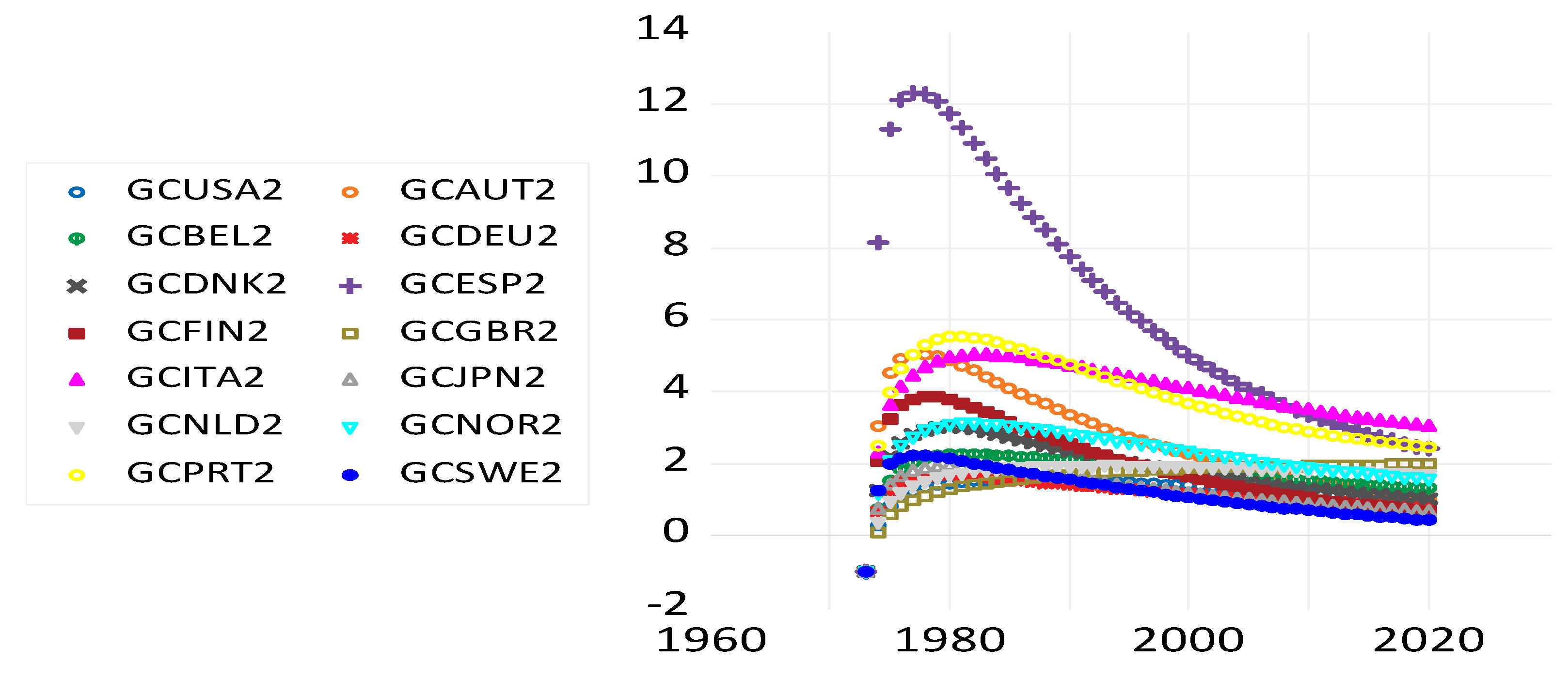
6. Public and Private R&D Changes

6.1. Effects from Enhancing Public R&D

A crucial question is whether a change in public R&D leads to more productivity and a higher GDP and effects on other R&D variables in line with Model 3 in Table 5 when taking into account all feedback effects from the VECM, which is a major difference compared to having just positive regression coefficients for public on private R&D and from R&D variables on labor-augmenting technical change. In this section, we show results from imposing a shock of 0.005 on each country’s intercept of the growth rate equation for public R&D, which is equivalent to a repeated one-time random shock.30 Figure 1 shows that the 14 countries gained up to 12.5% in labor-augmenting productivity in the 47 years between 1973 and 2020, which is 12.5/47 = 0.266 percent per year.

The percentage effect of a public R&D enhancement on the GDP, shown in Figure 2, is higher than that on technical change, shown in Figure 1. This may be due to a greater inflow (less outflow) of capital and labor. In the case of using only FMOLS of Model 1, the effects on productivity and GDP are slightly larger, 26 and 28 percent (see Appendix C); for pure DOLS of Model 2, they are 14 and 18 percent (see Appendix D), and in Figure 1 and Figure 2, they are 12.5 and 17.4 percent. The choice of Model 3, emphasizing cross-section independence, leads to the weakest effects.

Public and private R&D stock increases by up to almost 80 and 45 percent of baseline values are shown in Figure 3, and almost 80% and 60% for the DOLS Model 2 and slightly more than 100% and 55% for FMOLS Model 1 above baseline in Appendix C and Appendix D.

The results for Figure 1, Figure 2 and Figure 3 have been obtained with feedback from what the other countries are doing in terms of foreign public and private R&D in each country’s model. Figure 4 shows the (expected) foreign reactions, extending the result of Haskel and Wallis (2013) that domestic public R&D attracts foreign R&D to the UK, here for public and private foreign R&D separately for a panel of countries.

This result suggests positively sloped reaction curves for public and private R&D from the perspective of the Cournot oligopoly model of Cabon-Dhersin and Gibert (2020), for which positive international spillovers of public to private R&D are required for positively sloped reaction curves. Spillovers and strategic reactions are, therefore, hard to separate empirically.

In order to get a feeling whether the gains in terms of higher GDP outweigh the costs, we calculate the gains/GDP and the gains/cost ratio for every year. The yearly gross gains are the higher GDP of the policy scenario compared to baseline. The yearly costs stem from the differences in the domestic R&D stocks, requiring a higher net investment (plus higher depreciation a period later), again, with the scenario compared to the baseline. To approximate the costs roughly and in a simple manner, we take the percentage difference in the domestic public and private R&D stocks from Figure 3 and multiply them to the stock values of the baseline scenario, resulting in the investment difference required to obtain the higher value; a factor of 1.15 includes the depreciation costs. The net gains are the gross gains minus the costs. We divide the net gains either by the GDP or by the costs, which is a different rate of return measure than those in the literature, which has estimated parameters of production functions (see Hall et al. 2010) or internal rates of return (Soete et al. 2020; Ziesemer 2023b), which are discount rates that bring the sum of all discounted net gains to zero. If the flows of net gains are positive in all periods, internal rates of return are infinity. Therefore, utmost caution is required when comparing results for rates of return based on different concepts. Figure 5 shows that net gains are between 0 and 13% (0 and 21 percent of GDP for the FMOLS Model 1 and the DOLS Model 2; see Appendix B and Appendix C.

Figure 6 shows that net gains run up mostly from 0 to between beyond 500 percent of the yearly costs, ignoring the positive outliers of Spain (also for the FMOLS and DOLS models). The gains/cost ratios all start at a value of −1 because the first period has costs, but gains come only later.

Due to the nature of technical change, effects on the GDP are accumulating over time. Similarly, the differences in the stocks are built through investment over several years. These rough and simple calculations suffice to indicate that additional public R&D is advantageous in the 14 OECD countries, but they do not compare to any form of rate of return because they just divide the yearly gains and hypothetical costs or GDP by each other. Moreover, almost the same percentage changes shown in Figure 1, Figure 2, Figure 3 and Figure 4 lead to different gains as percentages of the cost or GDP for the countries because of different baseline levels.

6.2. Effects from Enhancing Domestic Private R&D, Foreign Private and Public R&D

A permanent change in the intercept of the equations for private R&D by 0.005 leads to negative effects on all variables (not shown) except private R&D itself up to 0.4, as well as a temporary small increase in foreign private (up to 0.0036) and domestic and foreign public R&D stocks (respectively, not higher than 0.002 and up to 0.001) in spite of the long-run relations shown in Table 5. Technical change and GDP go down, although long-term relations suggest that BERD should increase the productivity and GDP. These partial long-term effects are outweighed by system feedback effects and show that positive partial effects in a long-term relation are not sufficient support for policy suggestions. The results are in line with the finding of Luintel and Khan (2004), who demonstrate that the effect of business R&D is weaker than effects of total R&D, pointing to a strong role of public R&D. Similarly, Voutsinas and Tsamadias (2014) for Greece, Bengoa et al. (2017) for Spanish regions, Guellec and van Pottelsberghe de la Potterie (2003a), Luintel et al. (2014) and Herzer (2022) for an OECD country panel find that the effect of public R&D is stronger than that of private R&D in their regression coefficients. Intuitively, this could mean that private R&D is near its optimum, and additional private R&D then is driving the economies away from the optimum to lower levels. Alternatively, this is a result where the slope homogeneity assumption introduces a heterogeneity bias, if the cross-section variance of the slope coefficients is large and persistence is not (Rebucci 2010) (perhaps together with end-of-sample bias through the 2007–2013 crises), with an impact on the simulation results. This alternative interpretation is more in line with the single-country analyses for the Netherlands (Soete et al. 2020), USA and Japan in studies of Ziesemer (2022, 2024a), where additional private R&D has positive effects on productivity, requiring that other countries have much less favorable results in separate panel analyses than these three.

In contrast, the same change for foreign private R&D drives up all variables for all countries (not shown): BERD and foreign BERD from 0 to 160%, foreign public R&D to 92%, GDP to 82%, domestic public R&D by 240% and th07 by 216%.31 Percentages above 200 may seem unrealistic because they imply more than 4 percent for each year from 1973 to 2020. These numbers are similar for DOLS Model 2 and smaller in the case of FMOLS Model 1.

The same change for foreign public R&D drives up (not shown) domestic public R&D up to 0.6 beyond baseline. Domestic and foreign private R&D go down. Foreign public R&D goes up to 35% beyond baseline, and technical change goes up to 17.2% beyond baseline of th07. The GDP shows a positive effect, running up to 10.4% of the baseline. As domestic and foreign private R&D go down and productivity goes up, there must be a positive effect from domestic and foreign public R&D.

7. Conclusions

Our VECM approach of using four cointegrating equations shows favorable results for public R&D without resort to variables other than R&D, productivity, and GDP, whereas Khan and Luintel (2006) and van Elk et al. (2015, 2019) obtained comparable results through adding control variables from international public and innovation economics. By implication, the dependence of public R&D effects on national circumstances seems to be much weaker for our approach for the 14 OECD countries. The four long-term relations have support from (i) panel cointegration tests, (ii) cointegrating regressions using FMOLS and DOLS and (iii) shock (or impulse response) analysis for a panel VECM with four cointegrating equations. Distinguishing between direct and indirect effects of public R&D on productivity, as achieved in these VECMs, makes things economically a bit clearer and simpler. In the long-term relations, both the direct effects of public R&D on productivity and the indirect ones via private R&D are positive when using group mean FMOLS or DOLS estimation.

Using the panel VECM with (i) DOLS long-term relations for the GDP and technical change equations and (ii) the FMOLS equations for the private and public R&D equations, shocks to public R&D enhance private R&D, technical change and GDP growth. Shocks to foreign private and public R&D show that foreign private R&D has positive spillovers to technical change and all other variables, which are hard to distinguish from oligopolistic strategic reactions though (Ziesemer 2022). Foreign public and private R&D increase growth permanently. Using only FMOLS (see Appendix C) or only DOLS (see Appendix D) for the long-term relations changes some of these results but never the one for domestic public R&D. Increasing public R&D results in high net gains and is clearly a highly advantageous policy. However, we cannot exclude that governments have other highly advantageous policy opportunities for spending money or high costs and/or political resistance against raising taxes.

In VECMs, slope homogeneity, a limitation in the differenced part of the VECM, in general, may produce results with heterogeneity bias, and country-specific VECMs are most probably better in dealing with country-specific heterogeneity and policy, but they may suffer from small numbers of observations and, therefore, end-of-sample bias from recent crises. However, this does not affect the results of this paper regarding public R&D, whereas those for private R&D may be affected. Moreover, cross-section dependence is now dealt with through the use of mean-group estimation of the long-term relations, but not for the differenced parts, where the SURE method takes it into account in the estimation without addressing panel slope heterogeneity.

In future research, the issue of slope heterogeneity in adjustment coefficients and differenced terms can perhaps be explored. Panel VECM methods could benefit from aligning the approaches of panel VECM with the DOLS or FMOLS cointegrating equations lined up in Hsiao (2022) with those of the PMG/ARDL single-equation estimator of Pesaran et al. (1999). Whereas the VECM with DOLS or FMOLS cointegrating equations has mean-group slope estimation in the long-term relations and slope homogeneity in the differenced terms and adjustment coefficients, the PMG has the opposite: slope homogeneity in the estimation of only one long-term relation and mean-group estimation of differenced terms and adjustment coefficients. One such effort is the new system PMG estimator of Chudik et al. (2023) for pairs of variables and, by implication, only one long-term relation. This raises the question, which of the methods suffers more from slope heterogeneity bias and, so far, the restriction of the number of long-term relations to only one?

Another suggestion for future research is to estimate the time-varying elasticities of productivity. The statistical theory with evidence shows that functional coefficient regressions can indeed account for some data processes, but linear ar(2) and threshold autoregressive (ar) processes give remarkably comparable results (Chen and Tsay 1993; Cai et al. 2000). I.o.w. lags and threshold are substitutes for variable estimated coefficients. We use lags here and will use functional coefficient regression in the future.

For the time being, public R&D has positive direct and indirect (via private R&D) effects on productivity in DOLS and FMOLS estimates, and positive impulse response effects are shown when using the panel VECM with slope homogeneity, fixed effects and long-term relations from DOLS and FMOLS group mean estimations.

References

1. Abdih, Yasser, and Frederick Joutz. 2006. Relating the knowledge production function to total factor productivity: An endogenous growth puzzle. IMF Staff Papers 53: 242–71. [Google Scholar]
2. Adema, Yvonne, Paul Verstraten, and Bastiaan Overvest. 2023. Kwantificeren Economische Baten van R&D-Beleid. Den Haag: CPB Publication. [Google Scholar]
3. Ahn, Seung C., and Alex R. Horenstein. 2013. Eigenvalue ratio test for the number of factors. Econometrica 81: 1203–27. [Google Scholar]
4. Antolin-Diaz, Juan, and Paolo Surico. 2022. The long-run effects of government spending. In Discussion Paper DP17433. London: Centre for Economic Policy Research. [Google Scholar]
5. Arrow, Kenneth. J., Hollis. B. Chenery, Bagicha S. Minhas, and Robert M. Solow. 1961. Capital-labor substitution and economic efficiency. The Review of Economics and Statistics 43: 225–50. [Google Scholar]
6. Bai, Jushan, and Serena Ng. 2004. A PANIC attack on unit roots and cointegration. Econometrica 72: 1127–78. [Google Scholar]
7. Baltagi, Badi H. 2021. Econometric Analysis of Panel Data, 6th ed. Berlin: Springer. [Google Scholar]
8. Banerjee, Anindya, and Josep Lluís Carrion-i-Silvestre. 2017. Testing for panel cointegration using common correlated effects estimators. Journal of Time Series Analysis 38: 610–36. [Google Scholar]
9. Bassanini, Andrea, Philip Hemmings, and Stefano Scarpetta. 2001. Economic Growth: The Role of Policies and Institutions: Panel Data. Evidence from OECD Countries OECD Economics Department Working Papers No. 283. Available online: https://www.oecd-ilibrary.org/docserver/722675213381.pdf?expires=1724238970&id=id&accname=guest&checksum=D1BF24F31369E9325236A5DCBC7B77AF (accessed on 13 August 2024).
10. Bengoa, Marta, Valeriano Martínez-San Román, and Patrició Pérez. 2017. Do R&D activities matter for productivity? A regional spatial approach assessing the role of human and social capital. Economic Modelling 60: 448–61. [Google Scholar]
11. Branson, William H., and James M. Litvack. 1981. Macroeconomics, 2nd ed. New York: Harper&Row. [Google Scholar]
12. Breitung, Jörg. 2005. A Parametric Approach to the Estimation of Cointegration Vectors in Panel Data. Econometric Reviews 24: 151–73. [Google Scholar] [CrossRef]
13. Cabon-Dhersin, Marie-Laure, and Romain Gibert. 2020. R&D Cooperation, Proximity and Distribution of Public Funding Between Public and Private Research Sectors. The Manchester School 88: 773–800. [Google Scholar] [CrossRef]
14. Cai, Zongwu, Jianqing Fan, and Qiwei Yao. 2000. Functional-Coefficient Regression Models for Nonlinear Time Series. Journal of the American Statistical Association 95: 941–56. [Google Scholar]
15. Chen, Rong, and Ruey S. Tsay. 1993. Functional-Coefficient Autoregressive Models. Journal of the American Statistical Association 88: 298–308. [Google Scholar]
16. Chudik, Alexander, M. Hashem Pesaran, and Ron P. Smith. 2023. Revisiting the Great Ratios Hypothesis. Oxford Bulletin of Economics and Statistics 85: 1023–47. [Google Scholar] [CrossRef]
17. Ciaffi, Giovanna, Matteo Deleidi, and Enrico Sergio Levrero. 2023. The macroeconomic effects of public expenditure in research and development. In CIMR Research Working Paper No. 64. London: Birkbeck. [Google Scholar]
18. Coakley, Jerry, Ana-Maria Fuertes, and Ron Smith. 2002. A principal components approach to cross-section dependence in panels. Paper No. B5-3. Paper presented at the 10th International Conference on Panel Data, Berlin, Germany, July 5–6. [Google Scholar]
19. Coe, David T., and Elhanan Helpman. 1995. International R&D spillovers. European Economic Review 39: 859–87. [Google Scholar]
20. David, Paul A., and Brownwyn H. Hall. 2000. Heart of Darkness: Modeling Public–private Funding Interactions Inside the R&D Black Box. Research Policy 29: 1165–83. [Google Scholar]
21. David, Paul A., Bronwyn H. Hall, and Andrew A. Toole. 2000. Is public R&D a complement or substitute for private R&D? A review of the econometric evidence. Research Policy 29: 497–529. [Google Scholar]
22. De Lipsis, Vincenzo, Matteo Deleidi, Mariana Mazzucato, and Paolo Agnolucci. 2022. Macroeconomic Effects of Public R&D. Available online: https://ssrn.com/abstract=4301178 (accessed on 13 August 2024).
23. Deleidi, Matteo, and Mariana Mazzucato. 2021. Directed innovation policies and the supermultiplier: An empirical assessment of mission-oriented policies in the US economy. Research Policy 50: 104151. [Google Scholar]
24. Donselaar, Piet, and Carl Koopmans. 2016. The Fruits of R&D: Meta-Analyses of the Effects of Research and Development on Productivity. VU Amsterdam Research Memorandum 2016-1. Amsterdam: Faculty of Economics and Business Administration. [Google Scholar]
25. Elnasri, Amani, and Kevin J. Fox. 2017. The contribution of research and innovation to productivity. Journal of Productivity Analysis 47: 291–308. [Google Scholar]
26. Enders, Walter. 2015. Applied Econometric Time Series, 4th ed. New York: Wiley. [Google Scholar]
27. Erken, Hugo, Piet Donselaar, and Roy Thurik. 2008. Total factor productivity and the role of entrepreneurship. In Jena Economic Research Papers No. 2008,019. Jena: Friedrich Schiller University Jena, Max Planck Institute of Economics. [Google Scholar]
28. Erken, Hugo, Piet Donselaar, and Roy Thurik. 2018. Total factor productivity and the role of entrepreneurship. Journal of Technology Transfer 43: 1493–521. [Google Scholar] [CrossRef]
29. Estrada, Ángel, and José Manuel Montero. 2009. R&D Investment and Endogenous Growth: A SVAR Approach. Documentos de Trabajo N.° 0925. Madrid: BANCO DE ESPAÑA. [Google Scholar]
30. Falk, Martin. 2006. What drives business Research and Development (R&D) intensity across Organisation for Economic Co-operation and Development (OECD) countries? Applied Economics 38: 533–47. [Google Scholar]
31. Feenstra, Robert C., Robert Inklaar, and Marcel P. Timmer. 2015. The Next Generation of the Penn World Table. American Economic Review 105: 3150–82. [Google Scholar]
32. Fieldhouse, Andrew J., and Karel Mertens. 2023. The Returns to Government R&D: Evidence from U.S. Appropriations Shocks. Dallas: Federal Reserve Bank of Dallas. [Google Scholar]
33. Galor, Oded, and David N. Weil. 1999. From Malthusian Stagnation to Modern Growth. American Economic Review 89: 150–54. [Google Scholar]
34. Gandolfo, Giancarlo. 1971. Economic Dynamics: Methods and Models. Amsterdan: Elsevier, vol. 16. [Google Scholar]
35. Goolsbee, Austan. 1998. Does Government R&D Policy Mainly Benefit Scientists and Engineers? Working Paper No. 6532. Available online: https://www.nber.org/system/files/working_papers/w6532/w6532.pdf (accessed on 13 August 2024).
36. Groen, Jan J. J., and Frank Kleibergen. 2003. Likelihood-Based Cointegration. Analysis in Panels of Vector Error-Correction Models. Journal of Business & Economic Statistics 21: 295–318. [Google Scholar]
37. Guellec, Dominique, and Bruno Van Pottelsberghe de la Potterie. 2003a. R&D and Productivity Growth: Panel Data Analysis of 16 OECD Countries. OECD Economic Studies 2001/2: 103–26. [Google Scholar]
38. Guellec, Dominique, and Bruno Van Pottelsberghe de la Potterie. 2003b. The impact of public R&D expenditure on business R&D. Economics of Innovation and New Technology 12: 225–43. [Google Scholar]
39. Guellec, Dominique, and Bruno Van Pottelsberghe de la Potterie. 2004. From R&D to Productivity Growth: Do the Institutional Settings and the Source of Funds of R&D Matter? Oxford Bulletin of Economics and Statistics 66: 353–78. [Google Scholar]
40. Hall, Brownwyn H., Jacques Mairesse, and Pierre Mohnen. 2010. Measuring the Returns to R&D. In Handbook of the Economics of Innovation 2. Edited by Bronwyn H. Hall and Nathan Rosenberg. Amsterdam: Elsevier, pp. 1033–82. [Google Scholar]
41. Haskel, Jonathan, and Gavin Wallis. 2013. Public support for innovation, intangible investment and productivity growth in the UK market sector. Economics Letters 119: 195–98. [Google Scholar]
42. Helpman, Elhanan. 1992. Endogenous macroeconomic growth theory. European Economic Review 36: 237–67. [Google Scholar]
43. Herzer, Dierk. 2022. An empirical note on the long-run effects of public and private R&D on TFP. Journal of the Knowledge Economy 13: 1–17. [Google Scholar]
44. Hsiao, Cheng. 2022. Analysis of Panel Data, 4th ed. Cambridge: Cambridge University Press. [Google Scholar]
45. Huang, Chien Y., Ching Chong Lai, and Pietro F. Peretto. 2023. Public R&D, Private R&D and Growth: A Schumpeterian Approach. Available online: https://public.econ.duke.edu/~peretto/Public%20R&D%20and%20Growrh.pdf (accessed on 13 August 2024).
46. Inklaar, Robert, Pieter Woltjer, and Daniel Gallardo Albarrán. 2019. The Composition of Capital and Cross-country Productivity Comparisons. International Productivity Monitor 36: 34–52. [Google Scholar]
47. Jaumotte, Florence, and Nigel Pain. 2005a. From ideas to development: The determinants of R&D and patenting. In OECD Economics Department Working Paper No. 457. Paris: OECD. [Google Scholar]
48. Jaumotte, Florence, and Nigel Pain. 2005b. Innovation in the business sector. In OECD Economics Department Working Paper No. 459. Paris: OECD. [Google Scholar]
49. Jusélius, Katarina. 2006. The Cointegrated VAR Model: Methodology and Applications. Oxford: Oxford University Press. [Google Scholar]
50. Kao, Chihwa. 1999. Spurious Regression and Residual-Based Tests for Cointegration in Panel Data. Journal of Econometrics 90: 1–44. [Google Scholar]
51. Kao, Chihwa, and Min-Hsien Chiang. 2000. On the Estimation and Inference of a Cointegrated Regression in Panel Data. In Advances in Econometrics. Edited by B. Baltagi. Leeds: Emerald, vol. 15, pp. 161–78. [Google Scholar]
52. Kao, Chihwa, Min-Hsien Chiang, and Bangtian Chen. 1999. International R&D spillovers: An application of estimation and inference in panel cointegration. Oxford Bulletin of Economics and Statistics 61: 691–709. [Google Scholar]
53. Khan, Mosahid, and Kul B. Luintel. 2006. Sources of Knowledge and Productivity: How Robust Is the Relationship? Sti/Working Paper 2006/6. Paris: OECD. [Google Scholar]
54. Kilian, Lutz, and Helmut Lütkepohl. 2017. Structural Vector Autoregressive Analysis. Cambridge: Cambridge University Press. [Google Scholar]
55. Larsson, Rolf, and Johan Lyhagen. 2007. Inference in Panel Cointegration Models with Long Panels. Journal of Business & Economic Statistics 25: 473–83. [Google Scholar]
56. Lau, Sau-Him P. 1997. Using Stochastic Growth Models Unit Roots and Breaking Trends. Journal of Economic Dynamics and Control 21: 1645–67. [Google Scholar]
57. Loertscher, Oliver, and Pau S. Pujolas. 2024. Canadian Productivity Growth: Stuck in the Oil Sands. Canadian Journal of Economics 57: 478–501. [Google Scholar]
58. Lucas, Robert E., Jr. 2015. Human capital and growth. American Economic Review 105: 85–88. [Google Scholar]
59. Luintel, Kul B., and Mosahid Khan. 2004. Are international R&D spillovers costly for the United States? The Review of Economics and Statistics 86: 896–910. [Google Scholar]
60. Luintel, Kul B., Mosahid Khan, and Konstantinos Theodoridis. 2014. On the robustness of R&D. Journal of Productivity Analysis 42: 137–55. [Google Scholar]
61. Lütkepohl, Helmut. 2005. New Introduction to Multiple Time Series Analysis. Berlin: Springer Science & Business Media. [Google Scholar]
62. Maddala, Gangadharrao S., and Shaowen Wu. 1999. A Comparative Study of Unit Root Tests with Panel Data and A New Simple Test. Oxford Bulletin of Economics and Statistics 61: 631–52. [Google Scholar]
63. Moretti, Enrico, Claudia Steinwender, and John Van Reenen. 2023. The Intellectual Spoils of War? Defense R&D, Productivity, and International Spillovers. The Review of Economics and Statistics, 1–46. [Google Scholar]
64. Mukerji, Vatsala. 1963. A Generalized S.M.A.C. Function with Constant Ratios of Elasticity of Substitution. The Review of Economic Studies 30: 233–36. [Google Scholar]
65. OECD. 2017. The Impact of R&D Investment on Economic Performance: A Review of the econometric evidence. DSTI/STP/NESTI 2017 12. In Working Party of National Experts on Science and Technology Indicators. Paris: OECD Publishing. [Google Scholar]
66. Park, Walter G. 1995. International Spillovers of R&D Investment and OECD Economic Growth. Economic Inquiry 33: 571–91. [Google Scholar]
67. Park, Walter G. 1998. A theoretical model of government research and growth. Journal of Economic Behavior & Organization 34: 69–85. [Google Scholar]
68. Pedroni, Peter. 1999. Critical values for cointegration tests in heterogeneous panels with multiple regressors. Oxford Bulletin of Economics and Statistics 61: 653–70. [Google Scholar]
69. Pedroni, Peter. 2001a. Purchasing power parity tests in cointegrated panels. Review of Economics and Statistics 83: 727–31. [Google Scholar]
70. Pedroni, Peter. 2001b. Fully modified OLS for heterogeneous cointegrated panels. In Nonstationary Panels, Panel Cointegration, and Dynamic Panels. Leeds: Emerald Group Publishing Limited, vol. 15, pp. 93–130. [Google Scholar]
71. Pedroni, Peter. 2019. Panel cointegration techniques and open challenges. In Panel Data Econometrics. Cambridge: Academic Press, pp. 251–87. [Google Scholar]
72. Pegkas, Panagiotis, Christos Staikouras, and Constantinos Tsamadias. 2020. Does domestic and foreign R&D capital affect total factor productivity? Evidence from Eurozone countries. International Economic Journal 34: 258–78. [Google Scholar]
73. Perkins, Dwight. H., Steven Radelet, David L. Lindauer, and Steven A. Block. 2013. Economics of Development, 7th ed. New York: Norton. [Google Scholar]
74. Pesaran, M. Hashem. 2015. Time Series and Panel Data Econometrics. Oxford: Oxford University Press. [Google Scholar]
75. Pesaran, M. Hashem, Y. Shin, and Ron P. Smith. 1999. Pooled mean group estimation of dynamic heterogeneous panels. Journal of the American statistical Association 94: 621–34. [Google Scholar]
76. Pesaran, M. Hashem, and Yimeng Xie. 2023. A Bias-Corrected CD Test for Error Cross-Sectional Dependence in Panel Data Models with Latent Factors. arXiv arXiv:2109.00408. [Google Scholar]
77. Pesaran, M. Hashem. 2006. Estimation and Inference in Large Heterogeneous Panels with a Multifactor Error Structure. Econometrica 74: 967–1012. [Google Scholar]
78. Pesaran, M. Hashem. 2007. A Simple Panel Unit Root Test in the Presence of Cross-Section Dependence. Journal of Applied Econometrics 22: 265–312. [Google Scholar]
79. Ramanathan, Ramu. 2012. Introduction to the Theory of Economic Growth. Berlin: Springer Science & Business Media, vol. 205. [Google Scholar]
80. Rebucci, Alessandro. 2010. Estimating VARs with long stationary heterogeneous panels: A comparison of the fixed effect and the mean group estimators. Economic Modelling 27: 1183–98. [Google Scholar]
81. Rehman, Naqeeb Ur, Eglantina Hysa, and Xuxin Mao. 2020. Does public R&D complement or crowd-out private R&D in pre and post economic crisis of 2008? Journal of Applied Economics 23: 349–71. [Google Scholar]
82. Sato, Ryuzo. 1963. Fiscal Policy in a Neo-Classical Growth Model: An Analysis of Time Required for Equilibrating Adjustment. The Review of Economic Studies 30: 16–23. [Google Scholar]
83. Schwert, G. William. 1989. Stock Volatility and Crash of 87. Review of Financial Studies 3: 77–102. [Google Scholar]
84. Shanks, Sid, and Simon Zheng. 2006. Econometric Modelling of R&D and Australia’s Productivity. Staff Working Paper. Canberra: Productivity Commission. [Google Scholar]
85. Smith, Ron P., and Ana-Maria Fuertes. 2016. Panel Time-Series. London: V cemmap. [Google Scholar]
86. Soete, Luc, Bart Verspagen, and Thomas H. W. Ziesemer. 2020. The productivity effect of public R&D in the Netherlands. Economics of Innovation and New Technology 29: 31–47. [Google Scholar] [CrossRef]
87. Soete, Luc, Bart Verspagen, and Thomas H. W. Ziesemer. 2022. The economic impact of public R&D: An international perspective. Industrial and Corporate Change 31: 1–18. [Google Scholar] [CrossRef]
88. Solow, Robert M. 1956. A contribution to the theory of economic growth. The Quarterly Journal of Economics 70: 65–94. [Google Scholar]
89. Sveikauskas, Leo. 2007. R&D and Productivity Growth: A Review of the Literature; Working Paper 408. Washington, DC: U.S. Bureau of Labor Statistics.
90. Szirmai, Adam. 2011. Angus Maddison and development economics. In UNU-MERIT Working Papers No. 035. Maastricht: UNU-MERIT, Maastricht Economic and Social Research and Training Centre on Innovation and Technology. [Google Scholar]
91. van Ark, Bart, Klaas de Vries, and Dirk Pilat. 2024. Are pro-productivity policies fit for purpose? The Manchester School 92: 191–208. [Google Scholar]
92. van Elk, Roel, Bas ter Weel, Bart Verspagen, Karen van der Wiel, and Bram Wouterse. 2015. A Macroeconomic Analysis of the Returns to Public R&D Investments. CPB Discussion Paper 313. Maastricht: United Nations University—Maastricht Economic and Social Research Institute on Innovation and Technology (MERIT). [Google Scholar]
93. van Elk, Roel, Bas ter Weel, Karen van der Wiel, and Bram Wouterse. 2019. Estimating the returns to public R&D investments: Evidence from production function models. De Economist 167: 45–87. [Google Scholar]
94. van Pottelsberghe de la Potterie, Bruno, and Frank Lichtenberg. 2001. Does foreign direct investment transfer technology across borders? Review of Economics and Statistics 83: 490–97. [Google Scholar]
95. Voutsinas, Ioannis, and Constantinos Tsamadias. 2014. Does research and development capital affect total factor productivity? Evidence from Greece. Economics of Innovation and New Technology 23: 631–51. [Google Scholar]
96. Wagner, Martin, and Jaroslava Hlouskova. 2009. The performance of panel cointegration methods: Results from a large scale simulation study. Econometric Reviews 29: 182–223. [Google Scholar]
97. Wolff, Guntram B., and Volker Reinthaler. 2008. The Effectiveness of Subsidies Revisited: Accounting for Wage and Employment Effects in Business R&D. Research Policy 37: 1403–12. [Google Scholar] [CrossRef]
98. Wooldridge, Jeffrey M. 2013. Introductory Econometrics: A Modern Approach, 5th ed. Mason: Cencage Learning South Western. [Google Scholar]
99. Ziesemer, Thomas H. W. 2020. Japan’s productivity and GDP growth: The Role of private, public, and foreign R&D 1967–2017. Economies 8: 77. [Google Scholar] [CrossRef]
100. Ziesemer, Thomas H. W. 2021a. Semi-endogenous growth models with domestic and foreign private and public R&D linked to VECMs. Economics of Innovation and New Technology 30: 621–42. [Google Scholar] [CrossRef]
101. Ziesemer, Thomas H. W. 2021b. Mission-oriented R&D and growth. Journal of Applied Economics 24: 460–77. [Google Scholar] [CrossRef]
102. Ziesemer, Thomas H. W. 2021c. The effects of R&D subsidies and publicly performed R&D on business R&D: A survey. Hacienda Publica Espanola/Review of Public Economics 236: 171–205. [Google Scholar] [CrossRef]
103. Ziesemer, Thomas H. W. 2022. Foreign R&D spillovers to the USA and strategic reactions. Applied Economics 54: 4274–91. [Google Scholar] [CrossRef]
104. Ziesemer, Thomas H. W. 2023a. Labour-augmenting Technical Change Data for alternative Elasticities of Substitution: Growth, Slowdown, and Distribution Dynamics. Economics of Innovation and New Technology 32: 449–75. [Google Scholar] [CrossRef]
105. Ziesemer, Thomas H. W. 2023b. Internal rates of return for public R&D from VECM estimates for 17 OECD countries. In UNU-MERIT Working Paper 2023-026. Maastricht: UNU-MERIT. Available online: https://econpapers.repec.org/paper/unmunumer/2023026.htm (accessed on 12 August 2024).
106. Ziesemer, Thomas H. W. 2024a. Mission-oriented R&D and growth of Japan 1988–2016: A comparison with private and public R&D. Economics of Innovation and New Technology 33: 218–47. [Google Scholar] [CrossRef]
107. Ziesemer, Thomas H. W. 2024b. Evidence on an endogenous growth model with public R&D. Economics of Innovation and New Technology, 1–37. [Google Scholar] [CrossRef]
Figure 1. Effects on technical change (% TH07 baseline) through a shock of 0.005 of public R&D growth in 1973 for 14 OECD countries (14 lines visually ‘on’ each other).
Economies 12 00216 g001
Figure 2. Effects on GDP (% GDP baseline) from a shock of 0.005 of public R&D growth in 1973 for 14 OECD countries (14 remarkably similar lines ‘on’ each other).
Economies 12 00216 g002
Figure 3. R&D stock changes, with higher curves for public R&D and lower curves for private R&D, from a 0.005 increase in the intercept of the public R&D growth equation for each of the 14 countries. Public R&D runs up to about 80% above baseline and private R&D to 45%.
Economies 12 00216 g003
Figure 4. Foreign R&D reaction to a domestic public R&D enhancement. Higher curves are for foreign private R&D (up to 13.4%); lower curves are for foreign public R&D (up to 11.5%).
Economies 12 00216 g004
Figure 5. Yearly net gains as a percentage of the GDP, all in terms of the policy scenario compared to baseline.
Economies 12 00216 g005
Figure 6. Yearly net gains as a percentage of yearly costs, all in terms of the policy scenario compared to baseline.
Economies 12 00216 g006