Interrelationships Among Government Participation, Population and Growth of per Capita Income: Inquiry on Top Twenty Income-Holding Countries in the World

Abstract

The literature on growth in economics encompasses two main facets of thinking: the applicability of diminishing productivity of capital, as has been in the neoclassical growth model with exogenous technological progress, and the applicability of non-diminishing productivity of capital, as has been in the endogenous growth models. The main conclusion of the former is the cross-country convergence to a common steady state while that of the latter is non-convergence. The tremendous history of the growth of the world’s so-called developed economies in the 1980s, diverging with the so-called backward economies, has nullified the applicability of the neoclassical growth model and justified non-steady state positive per capita growth of income and consumption through endogenous technological progress in terms of knowledge capital, human capital, good public institutions, etc. The present study aims to examine whether per capita income growth is explained by the size of government intervention coupled with the working population size in the world’s top twenty countries in terms of aggregate income. With the theoretical setup of the model and using empirical tools, such as cointegration, error correction and causality in a vector autoregression structure, this study reveals that eighteen countries maintain long-run relationships among per capita income growth, government participation, population and the interaction factors between government intervention and population, excepting Germany and Canada. Further, in the short run, for eleven countries on the list, there are instances in which public institutions associated with the population and the interaction term have a causal influence on the growth of per capita income. The empirical results relating to income growth, thus, have sustainability implications.

1. Introduction

Economists often are engaged in a popular debate on whether the government sector should take part in economic activities. If yes, in what capacity? The classical (Smith, 1776; Say, 1834, among others) and neoclassical economists (Solow, 1956) had full faith in the working of a market economy in a competitive structure with the complete absence of the government sector as it hampers economic activity. Only the private buyers and sellers will be capable of determining commodity and factor prices with no sunk cost or dead weight loss. But the myth was broken in the 1920s when the world’s industrially developed market economies collapsed and there was a long recession in business activities. Classical economists had no solution at that time. The failure of the laissez faire doctrine of the capitalistic economists in the Great Depression of the 1920s and 1930s has been well known enough to allow public policymakers to promote government interventions in economic activities besides its social and administrative works—a phenomenon supported by the classical and neoclassical economists, philosophers and political scientists. In his General Theory, Professor J. M. Keynes (1936) recommended strong government interventions in economic activities, especially in the short run, to resist depressionary situations. Later, Robert Barro (1990) incorporated the government factor into the endogenous growth models to justify one of the major causes of why growth can be perpetual. But empirical evidence proves that government interventions may be good or bad for economies of different statures. The good effect channels are of two categories: first, the government must have a role in fields like legislation, security of property rights and providing a proper environment for private investment and production through decreasing transaction costs; second, the government must intervene in other fields where it comes to playing roles and/or giving services to sectors like infrastructures, human development, public health and education. The two alternatives support the forward linkage development policy where positive public investment leads to the expansion in the private sector and other associated sectors, leading to the applicability of the crowding-in hypothesis (Ramirez, 1998; Erden & Holcombe, 2006; Afonso & St. Aubyn, 2008; Mahmoudzadeh et al., 2013; Warner, 2014; Şen & Kaya, 2014; Das et al., 2015, 2018; Francois et al., 2024; among others). This hypothesis mostly works in the countries or groups of countries from developing nations where the capital markets are relatively underdeveloped compared to developed countries. The economic logic for defending government interventions in economic activities is that it protects the sectors in which the market mechanism fails or it has a comparative advantage over the private sector.

However, these interventions involve costs as well. Some of the propositions under this heading are as follows: First, the government has to afford its costs through public borrowing and tax revenues. Receiving taxes from economic agents makes them discouraged in that they reduce their work effort and consume and save less, which hurts economic growth. Second, public borrowing also increases the rate of interest and crowds out private investment and tax increases in the future (Aschauer, 1989; Furceri & Sousa, 2009; Phetsavong & Ichihashi, 2012; Şen & Kaya, 2014; Das et al., 2015, 2018; Nguyen & Trinh, 2018; Ben Zeev et al., 2023; among others). This happens mostly in the case of developed countries where capital markets are developed and have saturation levels depending on the requirements of the economies’ necessities; any more public investment leads to an increase in the rate of interest which leads to a reduction in the demand for investments from private units. Third, it produces inefficient economic outputs, unlike the market forces that bring the economy to optimality through the effective allocation of resources. Thus, government interventions, among others, can promote corruption and bureaucratic rent-seeking activities. Fourth, centralization and bureaucratic activities decrease creativity in both the public and private sectors. In accordance with market mechanisms, rewards and penalties of decisions are directly subject to wise choices, because they will appear in peoples’ wealth and property very soon. A series of positive and negative effects can be added to this.

Empirical evidence, including that provided by Grossman (1990), Ghali (1998), Loizides and Vamvoukas (2005), etc., reveals that the effect of government size is the cause of economic growth. On the other hand, studies such as those of Gwartney et al. (1998), Folster and Henrekson (2001), among others, reveal that the effect of government size on economic growth is negative. Furthermore, the theoretical works of Barro (1990), Mourmouras and Lee (1999), etc., and the empirical evidence provided by Barro (1991) and Chiou-Wei et al. (2010) show that in the lower levels of government activities, the effect of government expenditures is positive, but is reversed if it increases, which is shown with an inverted U-shaped curve.

Therefore, the activities of the government have both positive and negative effects on economic growth. On the one hand, it increases economic growth by providing a proper environment for private activities, legislation regarding private possession and its guarantee, building infrastructures and public goods, and on the other hand, it decreases economic growth through borrowing and taxation policies, decreasing creativity and increasing inefficiency, where the intensity of the negative effects depends on the amount of money spent and how it is spent (types of expenditures). Thus, the final effect of government expenditures depends on the kind of government expenditures (protection of property rights, subsidies, infrastructures, etc.) and its positive or negative effects on economic growth.

The role of the government sector in terms of good public institutions having public good properties in the growth of per capita income in the countries of the West during the 1980s onwards has been justified by an endogenous growth theoretician in the works of Barro (1990, 1991). The model establishes that the incorporation of a good public institution under no tax or a lump sum tax system causes the perpetual growth of per capita income and consumption and that these growth rates are dependent upon the size of government in the economy, the population size and the combinations of the two. Therefore, for countries, there should be long-term relationships between per capita income growth, the size of the government, population size and their interactions.

1.1. Objective of This Study

This study examines whether public sector participations in line with the endogenous growth model of Robert Barro have long-run relations with the per capita GDP growth rates in the world’s top 20 countries in terms of GDP for the period 1991–2020.

1.2. Contributions of This Study

This study contributes to the existing literature in the following manner:

• It examines the endogenous growth model involving public institutions for the world’s top 20 countries in GDP
• It incorporates the effects of population as a scale factor on growth of per capita GDP
• It captures the interaction effects between public participation and labor forces on per capita GDP growth rates and shows the route towards sustainable development

The paper is organized as follows: The next section, Section 2, presents the literature review followed by the theoretical model and public sector linkages with sustainable development. Section 3 focuses on the materials and methods; Section 4 covers results, analysis and discussion; and finally, Section 5 concludes this study.

2. Review of Related Literature

This study has conducted a literature review of the extant literature and classified it into three sub-sections. First, it covers the studies on the linkages between public spending and growth; then, it presents the theoretical model of Barro (1990) with some modifications in line with the requirements of this study; and then, it covers some studies on the public sector’s linkages with sustainable development.

2.1. Public Spending and Growth Linkages

Landau (1983) studied the relevant data of 104 countries on a cross-sectional basis and found significantly negative relations between the growth rate of real per capita GDP and the amount of government consumption expenditure as a ratio to GDP. Using data for each country averaged over roughly 20-year periods for 47 countries, Kormendi and Meguire (1985) found no significant relation between the average growth rates of real GDP and average growth rates or levels of the share of government consumption spending in GDP. Grier and Tullock (1987) extended the Kormendi–Meguire form of analysis to 115 countries, using data on government consumption for a pooled cross-section analysis, and found a significantly negative relation between the growth of real GDP and the growth of the government share of GDP. Barth and Bradley (1987) found a negative relation between the growth rate of real GDP and the share of government consumption spending for 16 OECD countries for the period 1971–1983. Aschauer (1989) argued that the services from government infrastructure were particularly important in the context of growth where the roles of public services as an input to private production were considered. It is this productive role that creates a potentially positive linkage between government and income growth. Barro (1989) showed that in the set of 98 countries for which government consumption spending to GDP was measured, a regression of the average annual growth rate of real per capita GDP from 1960 to 1985 on a set of explanatory variables led to negative coefficients. There was thus an indication that an increase in resources devoted to nonproductive (but possibly utility-enhancing) government services was associated with lower per capita growth rates of income. But with a separate set of 76 countries having the public-investment-to-GDP ratio as the regressor, the findings showed a positive coefficient. This result was consistent with the hypothesis that the typical country came closer to the quantity of public investment that would maximize the income growth rate. The role of government institutions, including the rule of law and well-functioning property rights, in explaining long-run economic performance has emerged from new institutional economics pioneered by North (1989). Devarajan et al. (1996) focus on the link between the level of public expenditure and growth using data from 43 developing countries over 20 years and show that an increase in the share of current expenditure has positive and statistically significant growth effects. Blankenau and Simpson (2004) explore this expenditure–growth relationship in the context of an endogenous growth model in which private and public investment are inputs to human capital accumulation, and the empirical evidence is mixed concerning the effects of public education expenditures on economic growth. Bose et al. (2007) examine the growth effects of government expenditure for a panel of 30 developing countries in the 1970s and 1980s in aggregate and disaggregated government expenditures. The results show that the share of government capital expenditure in GDP is positively and significantly correlated with economic growth, and at the disaggregated level, government investment in education and total expenditures in education are significantly associated with growth. Rajkumar and Swaroop (2008) examined the role of governance in the effectiveness of public spending in achieving social outcomes for a sample of 91 countries and showed that the quality of governance could largely explain differences in the efficacy of public spending. Afonso and Jalles (2011) conducted an empirical analysis of 108 countries for 1970–2008 on government size and institutional quality and found that the size of the government had an adverse effect on economic growth while institutional quality had a positive impact. Wu et al. (2010) examined the causal relationship between government expenditure and economic growth in a panel of 182 countries for 1950–2004 and found that the government played a role in economic growth. Afonso and Furceri (2010) analyzed the effects in terms of size and volatility of government spending and revenue on economic growth in OECD and EU countries and found both variables to be detrimental to economic growth. In their later study, Afonso and Jalles (2014) studied the fiscal composition–growth nexus for a set of OECD countries and found no significant impact of revenues on growth, whereas expenditures had negative effects. In their work, Chakraborty and Krishnankutty (2012) focus on the expenditure on education as a determinant of economic growth in Indian states. Using a panel data model, their study shows that expenditure on education positively influences the growth of the economy. Kurt (2015) investigates the direct and indirect effects of health expenditures on economic growth using the Feder–Ram model for Turkiye in monthly data for the period 2006–2013 and shows that the direct impact of government health expenditures on economic growth in Turkiye is positive and significant and its indirect impact is negative and significant. Malesevic and Golem (2019) obtained the results for EU15 countries during 1995–2014, where the single most important government expenditure item was education among aggregate expenditure for economic growth. Pahlevi (2017), studying an Indonesian panel of 33 states for the period 2008–2012, shows that governance and health expenditure are found to have a positive impact on human development; meanwhile, health expenditure is discovered to affect human development in a negative direction. Churchill et al. (2015) performed a hierarchical meta-regression analysis to review 87 empirical studies that report 769 estimates for the effects of government size on economic growth, and the findings indicate that the relationship between government size and growth is context-specific and the existing evidence is insufficient to establish a negative causal effect. Bhanumurthy et al. (2016) examined public expenditure, good governance and human development in districts of Madhya Pradesh in India, incorporating an interaction term to address the linkage effect of government expenditure; good governance was introduced in addition to other explanatory variables, and the result showed that good governance significantly contributed to better economic performance. Liu et al. (2018) conducted a study on governance quality and economic growth for provinces in China for the period 2001–2015 in a panel data model, and this study affirms that good governance contributes to growth positively. Olaoye et al. (2019) tested for causality between government expenditure and economic growth, but their result shows no evidence of a causal relationship. A list of studies was compiled by Das (2021) in a volume covering the debate on the optimum size of a government intervention which shows in general that the impact depends on several situations across countries and groups; however, no specific conclusion is drawn. Datta and Chakrabarti (2021) show that a government’s budget allocation for development management programs has an optimum level/upper bound negating the confusing results of the impacts on the size of the government intervention as evidenced by many studies in the literature. Sinha et al. (2021) highlight that the extent of FDI inflows is highly influenced by several macro policies of governments other than subsidies; however, government policies towards open economy macroeconomic factors are more effective. Jain and Nagpal (2021) have observed that a rise in the size of the public spending in a selected developing countries and groups results in a substantial increase (decrease) in the growth rate when the public spending is below (above) the optimal threshold level, indicating a non-monotonic association.

2.2. Theoretical Model

The weak justification of neoclassical economists such as Solow (1956) on the working of cross-country convergences during the 1980s among the developed nations has influenced the new growth theoreticians such as Rebelo (1991), Lucas (1988), Romer (1994), Ramsey (1928) and Barro (1990), who explained through endogenous growth models how the cross-country convergences did not work. The endogenous growth theories consider the working of increasing returns to scale where the sources of such returns to scale are research and development (the Romer Model), human capital (the Lucas Model), one-factor model (the Rebelo Model with Y = AK type production function) and good public institutions (the Barro Model).

The present study uses the basic structure of the Barro (1990) model of endogenous growth and makes some simple modifications of the production function incorporating the interaction effects between government expenditure as a ratio to aggregate output and the working population in the economy. This is because a good public institution (as measured by high G/Y) leads to good-quality public institutional outputs in terms of good educational attainment, health benefits, legal and judicial supports, internal and external security, etc., increasing the good-quality population size.

Thus, following the Barro model, let us suppose that, in the production function, there is G as the additional input (to represent public services or public input without congestion effects and user charges) with L and K (as private inputs) producing output Y. The Cobb–Douglas-type production function for the whole economy is

Y_i = AL^1−α. K^α. G^1−α

(1)

where 0 < α < 1.

The production function shows the working of constant returns to scale (CRS) in private inputs, L and K (as the sum of their powers is 1), and the inclusion of G as another factor of production leads the total production system to increasing returns to scale (IRS) as the sum of their powers is greater than 1. ‘A’ stands for technology which, among others, captures the interaction effects between government’s participation in the aggregate economy as measured by G/Y and L (the working population) which is G/Y × L (i.e., A = A(G/Y × L)). If all other components of A are fixed, then there can be a one-to-one relation between A and G/Y × L, i.e., A = (G/Y) × L. The modified model in the present study, thus, has more flexibility in analyzing the impacts of several components of the public institutional system on economic growth.

Assume that the aggregate labor force is constant. In that case, if G is constant, the returns from private capital (K) will be diminishing. On the other hand, if G increases along with K (that means both private and public capitals move in positive directions simultaneously like crowding-in effects), then diminishing MPk will not arise. Here, public capital is complementary to K and L and an increase in G leads to an increase in the MPL and MPk (this is the source of endogenous growth).

The production function in per capita form is

y = A. k^α. G^1−α

(2)

The total output of the economy is

Ʃy = y × L = Y = AL. k^α. G^1−α = AL. k^α. (G/G^α)
Or, G^α = (AL. k^α. G)/Y = AL. k^α. (G/Y)
   Or. G = (G/Y)^1/α. (AL)^1/α. k

(3)

The common budget constraint faced by the aggregate economy is

dk/dt = dm/dt = ṁ = y − c − δk − G/L

where G/L is per capita consumption of public goods/services. Here, ‘m’ is the state variable representing asset value, and c is the per capita consumption, which is the inverse of savings in an intertemporal infinite period model.

Following the Ramsey model, we set the current value Hamiltonian function for utility maximization with respect to c, G and k.

H = u(c_t). e^−(ρ−n)t + β_t [y − c − δk − G/L]

Here, β_t is the co-state variable, ρ is the discount rate, n is the population growth rate and δ is the rate of depreciation. Assuming the population growth rate is at n and the constant elasticity of substitution utility function, u = (c^1−σ/1 − σ), σ being the intertemporal elasticity of substitution or constant elasticity of marginal utility of consumption. Thus, the Hamiltonian is now

H(c, G, k) = (c^1−σ/1−σ). e^−(ρ−n)t + β_t[y − c − δk − G/L]

or, H(c, G, k) = (c^1−σ/1−σ). e^−(ρ−n)t + β_t[A. k^α. G^1−α − c − δk − G/L]

The FOCs are

δH/δc = 0,     >> c^−σ. (1−σ)/(1−σ). e^−(ρ−n)t = β

(4)

δH/δG = 0,     >>(1−α). β. A. k^α. G^−α − β/L = 0
          or, (1−α). A. k^α. G^−α = 1/L

(5)

δH/δk = −δβ/δt    >>β.α. A. k^α−1. G^1−α − β δ = −δβ/δt

(6)

And the transversality condition is

$$\underset{t\to \infty }{\lim }\left({\mathsf{\beta }}_t.{\mathrm{m}}_t\right)=0$$

Now, we take the derivative of β w.r.t time from (4) and substitute it into (6).

We obtain

β (α. A. k^α−1. G ^1−α− δ) = σ.c^−σ. [(δc/δt)/c]. e^−(ρ−n)t

Now, putting the value of β from (1) into the above relation

c^−σ. (1−σ)/(1−σ). e^−(ρ−n)t.(α. A. k^α−1. G^1−α − δ) = σ.c^−σ. [(δc/δt)/c]. e^−(ρ−n)t
         or, α. A. k^α−1. G^1−α − δ = σ. [(δc/δt)/c]
       or, [(δc/δt)/c] = 1/σ [α. A. k^α−1. G^1−α − n − δ]

(7)

Now, from (2),

(1−α). A. k^α. G^−α = 1/L
Or, (1−α). A. k^α. G^1−α = 1/L
Or, (1−α). A. L. k^α. G^1−α = 1
Or. (1−α). Y = G
    Or, G/Y = (1 − α)

(8)

This means the government-expenditure-to-GDP ratio (=G/Y) is constant where G/Y stands for the share of productive government expenditures in GDP. In other words, the optimal condition of the government in a country is to maintain a constant G/Y in the model with a lump sum tax. However, the shares vary across the countries depending upon the values of α, which measures the productivity of public services relative to private services. It could vary across countries for a number of reasons related to geography, the share of agricultural production, urban density and so on. Hence, the growth rates of income, consumption and capital accumulation vary across the countries. As the value of α increases, G/Y falls, and as a result, the growth rate falls.

Now, we put the expression of G from (1) in (7)

(δc/δt)/c = 1/σ [α. A. k^α−1. G^1−α − n − δ]
Or, (δc/δt)/c = 1/σ [α. A. k^α−1. G^1−α − n − δ]
Or, (δc/δt)/c = 1/σ [α. A. k^α−1. {(G/Y)^1/α. (AL)^1/α. k}^1−α − n − δ]
Or, (δc/δt)/c = 1/σ [α. A. k^α−1. {(1−α)^1−α/α. (AL)^1−α/α. k^1−α − n − δ]
Or, (δc/δt)/c = 1/σ [α. A^1/α. (1−α)^1−α/α. L^1−α/α − n − δ]

(9)

Therefore, the social planner’s optimum solution is identical to that under a decentralized system under the lump sum tax assumption.

The optimal rate of growth of k, y and c will be the rate [writing (δc/δt)/c = $\dot{{\displaystyle \frac{c}{c}}}$], which is given below as

ċ/c = 1/σ[α.A^1/α. (G/Y)^1−α/α. L^1−α/α − n − δ]
= 1/σ [α.A^1/α. (1−α)^1−α/α. L^1−α/α − n − δ]

Let us replace the term A with G/Y × L = (1 − α) × L (as has been explained in the introductory part of the model), and the revised consumption growth relation becomes

ċ/c = 1/σ [α. {(1−α) × L}^1/α. (1−α)^1−α/α. L^1−α/α − n − δ]          
          = 1/σ [α. (1−α)^(2−α)/α. L^(2−α)/α − n − δ]

(10)

It is clear from the expression that the rate of growth of per capita consumption depends on the marginal productivity of per capita capital which again depends upon the endogenous growth component, the G/Y ratio (=1 − α), population size (=L) and the interactions between G/Y and population size (captured by A = G/Y × L), but not on per capita capital accumulation (=k). The intuition behind the effects of G/Y on population or the reverse is that a good public institution (as measured by high G/Y or high (1 − α)) leads to good-quality public institutional outputs in terms of good educational attainment, health benefits, legal and judicial supports, internal and external security, etc., increasing the good-quality population size (Lucas, 1988; Barro & Lee, 1993; Barro, 2001; Barro & Lee, 2001; Verhulst, 1838; Das & Mukherjee, 2019; Diebolt & Hippe, 2019; Das, 2020; Hussain & Das, 2024). On the other hand, in countries having good-quality public institutions, the increase in population size of the countries will be able to absorb the good public institutional frameworks that will push up their productivity which will then help in increasing the growth of per capita consumption. The rate of growth of per capita income ($\dot{y}$/y) will then be positive with G/Y, population and their interaction term (G/Y × L). Hence, as the scale factor, L, increases along with G/Y, the marginal productivity of capital increases, breaks its diminishing nature, and ultimately, $\dot{c}$/c and $\dot{y}$/y increase in the long run without reaching any steady-state solution.

2.3. Public Sector Linkages with Sustainable Development

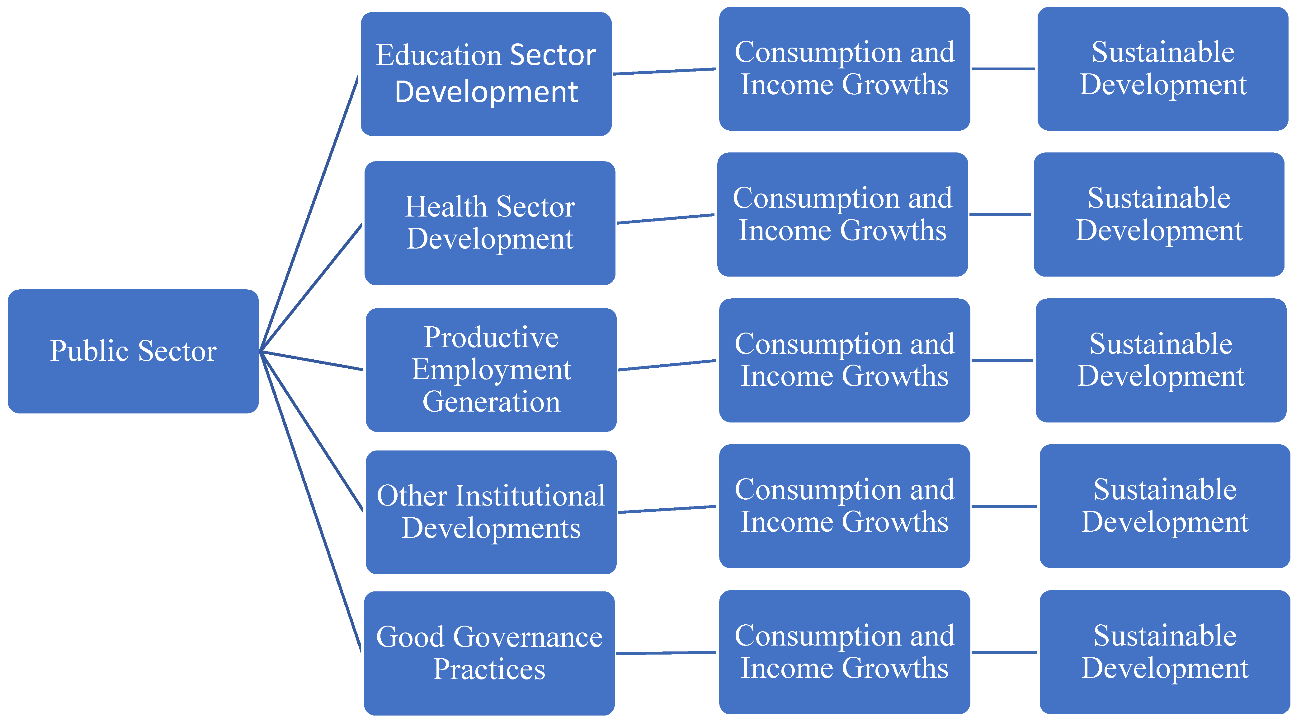
The United Nations 17-point sustainable development goals (SDGs) include good public institutions having the capability of making economic growth, promoting good health and education, reducing corruption, crimes, etc., which is covered in Goal Number 16. SDG 16 (Global Goal 16) is framed to promote peaceful and inclusive societies for sustainable development; provide access to justice for all; and build effective, accountable and inclusive institutions at all levels. The goal has 12 targets, 23 indicators and 10 outcome targets. The outcome targets related to our analysis are to develop effective, accountable and transparent institutions; ensure responsive, inclusive and representative decision-making; ensure public access to information; and protect fundamental freedoms. The proposed two means of implementation targets are strengthening national institutions to prevent violence and combat crime and terrorism and promoting and enforcing non-discriminatory laws and policies. In addition, SDGs 8, 9 and 12 are relevant to the present study. SDG 8 aims to promote sustained, inclusive and sustainable economic growth; full and productive employment; and decent work for all. SDG 9 aims to build resilient infrastructure, promote inclusive and sustainable industrialization, and foster innovation. SDG 12 aims to ensure sustainable consumption and production patterns. To ensure all such related goals are effective, the governments of countries need to spend a sizable amount from their budgets in order to promote education, health, good labor force development, consumption, economic growth and development. Hence, public sector spending is an important endogenous source of growth of a country. Figure 1 gives a preliminary sketch of the networking from public sector developments to consumption and income growth and sustainable development via different sectors as given in the five boxes in the second column.

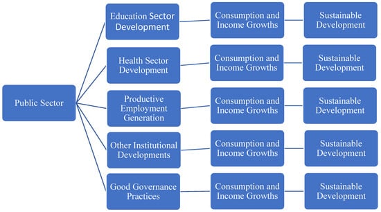
Figure 1. The networking from public sector developments to growth and sustainable development. Source: sketched by the author.

There is a list of studies that deal with public sector indicators and good governance indicators and their relations with growth and sustainable development in countries and regions. Barrett and Graddy (2000) observed that civil and political freedoms under the presence of some pollution variables strongly improve environmental quality, justifying countries’ positions along the downhill zone of the Environmental Kuznets Curve and thus signifying the attainment of SDGs. Glass and Newig (2019) examine the influence of different aspects of governance, notably, participation, policy coherence, reflexivity, adaptation and democratic institutions, on the achievement of SDGs at the national level, controlling additional socio-economic conditions, and found that democratic institutions and participation as well as economic power, education and geographic location serve to explain SDG achievement. Bolton (2021) revealed that public sector factors such as legislative and institutional structures, leadership and public decisions are recognized as a necessary catalyst for the achievement of the SDGs within Victoria in Australia. There are other related works on public sector governance and sustainable development such as those of Charron and Lapuente (2010); International Monetary Fund (2002); Meng (2024); etc.

The existing literature as mentioned above depicts the mixed results on the efficacy of government expenditure on the provisioning of public institutions and the public sector’s role in growth and sustainable development. However, no study considers the effects of the size of public participation coupled with population and their interaction effects on the growth of per capita GDP in world’s top countries in terms of aggregate GDP. The present study intervenes in this area.

3. Materials and Methods

3.1. Data Description

This study has considered the top 20 countries in the list of aggregate GDP as per the IMF classification. The countries in the ranking are the USA, China, Japan, Germany, India, the UK, France, Italy, Canada, Brazil, Russia, South Korea, Australia, Mexico, Spain, Indonesia, the Netherlands, Saudi Arabia, Turkiye and Switzerland. The three indicators are growth of per capita GDP, total government expenditure (both capital and revenue accounts) as a ratio to GDP (=G/Y) and population (L) aged 15–64 years. The interaction effects between G/Y and L are captured by the term G/Y × L. The data on GDP and government expenditures are measured in the current US dollar (USD). As the data on G/Y for both the capital and revenue accounts are not available from the source, this study has computed the public capital formation by deducting total private capital formation from the total capital formation. Then, the G/Y from the capital accounts is computed and is added to the revenue-expenditure-to-GDP ratio which is available from the source. The data on the population in the age group of 15–64 years are available in percentage form, and they are converted to total working-age population by multiplying the share by the total population. The total period of this study is 1991–2020 as the data on Russia are available from the year of 1991. The data source for GDP and population is the World Bank (www.worldbank.org), and that for private and public spending is the OECD (https://www.oecd.org/en/data.html, accessed on 25 December 2024).

3.2. Empirical Methodology

As this study has 30 data points, there may be stochastic trends, and to proceed with the cointegration and causality exercise, it is required to test for stationarity or the absence of unit roots of the four series for all the selected countries. The augmented Dickey and Fuller (1979) test is used for stationarity test. For the dataset of a variable, say y (y_t, t = 1, 2, …, T), where t denotes time, let us consider the following linear regression setup for unit root test for two versions of the ADF(p) regression:

$$\Delta y_t=\alpha +\beta y_{t-1}+\sum _{j=1}^p{\gamma }_j\Delta y_{t-j}+u_t$$

(11)

for the case without a time trend and

$$\Delta y_t=\alpha +\delta \mathrm{t}+\beta y_{t-1}+\sum _{j=1}^p{\gamma }_j\Delta y_{t-j}+u_t$$

(12)

for the case with a time trend.

If β = 0 is rejected by the ADF statistic in both specifications, then the series is said to be stationary. If this feature holds for all the series of growth of per capita GDP (PCGDP Growth), G/Y, L and G/Y × L, then regression can be run without the chances of obtaining spurious results. If not, we need to test whether the series are integrated of order one (I(1)) or first-difference stationary. If we obtain the result that all the series are I(1) (that is, integrated of the same order), then cointegration among the series can be tested to establish long-run relations. Since this study has four endogenous variables, the vector autoregression (VAR) model is used, and if the cointegration among them is found, then the vector error correction model (VECM) is applied to check the stability of the long-run relations. If the VECM term turns out to be negative and statistically significant, then the long-run relation is said to be stable or convergent; in addition, it is said that there are long run causalities running from any three independent variables to any one dependent variable out of the set of four. Further, it is required to test for short-run causality in line with Wald test to see whether there are causal influences from any three indicators to the other one in the list.

Let us structure a VAR model for four endogenous variables such as per capita GDP (PCGDP), the government participation rate (G/Y), the working population (L) and the interaction term (G/Y × L) which is given as the following set of equations:

$$PCGD{P}_t={\alpha }_1+{\displaystyle \sum _{j=1}^n{\beta }_{1j}PCGD{P}_{t-j}}+{\displaystyle \sum _{j=1}^n{\gamma }_{1j}{(G/Y)}_{t-j}}+{\displaystyle \sum _{j=1}^n{\delta }_{1j}{L}_{t-j}}+{\displaystyle \sum _{j=1}^n{\theta }_{1j}{(G/Y\times L)}_{t-j}}+u_{1t}$$

(13)

$${(G/Y)}_t={\alpha }_2+{\displaystyle \sum _{j=1}^n{\beta }_{2j}PCGD{P}_{t-j}}+{\displaystyle \sum _{j=1}^n{\gamma }_{2j}{(G/Y)}_{t-j}}+{\displaystyle \sum _{j=1}^n{\delta }_{2j}{L}_{t-j}}+{\displaystyle \sum _{j=1}^n{\theta }_{2j}{(G/Y\times L)}_{t-j}}+u_{2t}$$

(14)

$$L_t={\alpha }_3+{\displaystyle \sum _{j=1}^n{\beta }_{3j}PCGD{P}_{t-j}}+{\displaystyle \sum _{j=1}^n{\gamma }_{3j}{(G/Y)}_{t-j}}+{\displaystyle \sum _{j=1}^n{\delta }_{3j}{L}_{t-j}}+{\displaystyle \sum _{j=1}^n{\theta }_{3j}{(G/Y\times L)}_{t-j}}+u_{3t}$$

(15)

$${(G/Y\times L)}_t={\alpha }_4+{\displaystyle \sum _{j=1}^n{\beta }_{4j}PCGD{P}_{t-j}}+{\displaystyle \sum _{j=1}^n{\gamma }_{4j}{(G/Y)}_{t-j}}+{\displaystyle \sum _{j=1}^n{\delta }_{4j}{L}_{t-j}}+{\displaystyle \sum _{j=1}^n{\theta }_{4j}{(G/Y\times L)}_{t-j}}+u_{4t}$$

(16)

where the growth of PCGDP is shortly written as PCGDP, and α₁, β_1j, γ_1j, δ_1j, θ_1j stand for the intercept and slope coefficients when PCGDP Growth is the dependent variable. The notations with numbers will change accordingly from 2 to 4 for (G/Y), L and (G/Y × L) as the dependent variables. Once the optimum lag is selected, then the VAR model will have to be modified. If, for example, the optimum lag is 2, then the values of j will be 1 and 2.

After the cointegration test is performed, here, in line with the Johansen technique, the modeling of the VECM is performed to check the stability of such long-run relations. The VECM is a restricted VAR model, and it has a cointegrating relation built into the specification so that it restricts the long-run behaviors of the endogenous variables to converge to their long-run equilibrium relations while allowing for the short-run dynamics. The cointegrating term is known as the error correction (EC) term since the deviation from the long-run equilibrium is corrected gradually through a series of short-run dynamic adjustments. Here, the primary objective is to add estimated error terms with lagged values as the error correction terms. The VECM is given by the following set of equations:

$$\Delta PCGD{P}_t={\alpha }_1+{\displaystyle \sum _{j=1}^n{\beta }_{1j}\Delta PCGD{P}_{t-j}}+{\displaystyle \sum _{j=1}^n{\gamma }_{1j}\Delta {(G/Y)}_{t-j}}+{\displaystyle \sum _{j=1}^n{\delta }_{1j}\Delta L_{t-j}}+{\displaystyle \sum _{j=1}^n{\theta }_{1j}\Delta {(G/Y\times L)}_{t-j}}+{\displaystyle \sum _{i=1}^m\widehat{{\eta }_{1i}{e}_{1,t-i}}}+{\epsilon }_{1t}$$

(17)

$$\Delta {(G/Y)}_t={\alpha }_2+{\displaystyle \sum _{j=1}^n{\beta }_{2j}\Delta PCGD{P}_{t-j}}+{\displaystyle \sum _{j=1}^n{\gamma }_{2j}\Delta {(G/Y)}_{t-j}}+{\displaystyle \sum _{j=1}^n{\delta }_{2j}\Delta L_{t-j}}+{\displaystyle \sum _{j=1}^n{\theta }_{2j}\Delta {(G/Y\times L)}_{t-j}}+{\displaystyle \sum _{i=1}^m\widehat{{\eta }_{2i}{e}_{2,t-i}}}+{\epsilon }_{2t}$$

(18)

$$\Delta L_t={\alpha }_3+{\displaystyle \sum _{j=1}^n{\beta }_{3j}\Delta PCGD{P}_{t-j}}+{\displaystyle \sum _{j=1}^n{\gamma }_{3j}\Delta {(G/Y)}_{t-j}}+{\displaystyle \sum _{j=1}^n{\delta }_{3j}\Delta L_{t-j}}+{\displaystyle \sum _{j=1}^n{\theta }_{3j}\Delta {(G/Y\times L)}_{t-j}}+{\displaystyle \sum _{i=1}^m\widehat{{\eta }_{3i}{e}_{3,t-i}}}+{\epsilon }_{3t}$$

(19)

$$\Delta {(G/Y\times L)}_t={\alpha }_4+{\displaystyle \sum _{j=1}^n{\beta }_{4j}\Delta PCGD{P}_{t-j}}+{\displaystyle \sum _{j=1}^n{\gamma }_{4j}\Delta {(G/Y)}_{t-j}}+{\displaystyle \sum _{j=1}^n{\delta }_{4j}\Delta L_{t-j}}+{\displaystyle \sum _{j=1}^n{\theta }_{4j}\Delta {(G/Y\times L)}_{t-j}}+{\displaystyle \sum _{i=1}^m\widehat{{\eta }_{4i}{e}_{4,t-i}}}+{\epsilon }_{4t}$$

(20)

where $\widehat{e_{t-i}}$ is the lagged value of the estimated residuals and η$\widehat{e_{t-i}}$ is the error correction term. ‘η’ indicates the coefficient of EC, it is desirable for this value to be negative and statistically significant to establish the long-run associations among the variables.

Short-run causality, say in Equation (7), from (G/Y), L and (G/Y × L) to PCGDP Growth can be examined on the basis of testing the null hypothesis, H₀: γ_1j = δ_1j = θ_1j = 0. If the null hypothesis is accepted with probability values less than 0.05, then there is no causal influence occurring from (G/Y), L and (G/Y × L) to PCGDP Growth. The Wald test ensures the results.

4. Empirical Results and Analysis

4.1. Graphical View of the Trends of the Data Series

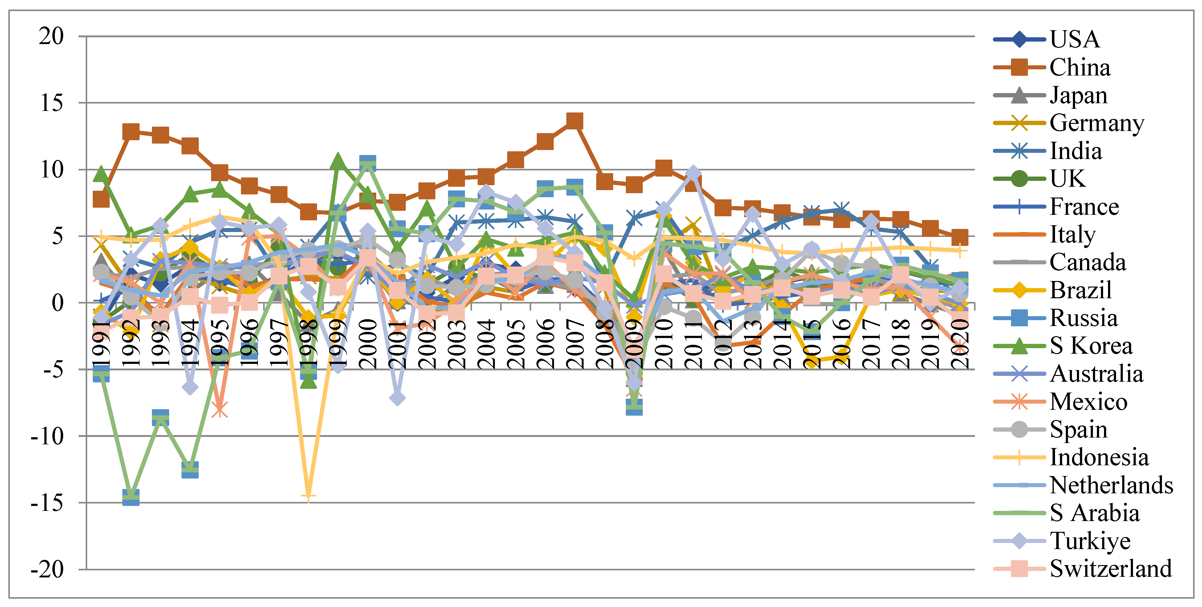
A graphical presentation provides a brief scenario of the selected indicators, and it is helpful to read the movements of the indicators over time. Figure 2, Figure 3, Figure 4 and Figure 5 present the trends of the indicators of PCGDP Growth, G/Y, population and the interaction term (G/Y × L), respectively, for the selected countries for the period 1991–2020. It is observed from Figure 2 that the countries from the list of developing countries like China, India, Turkiye, Indonesia, etc., maintain relatively higher growth rates in PCGDP and the world’s so-called developed countries stay behind the former. There are, however, fluctuations in the trends for all, making them nonstationary.

Figure 2. Trends of the PCGDP Growth rates of the countries. Source: drawn by the author.

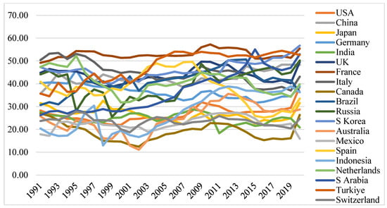
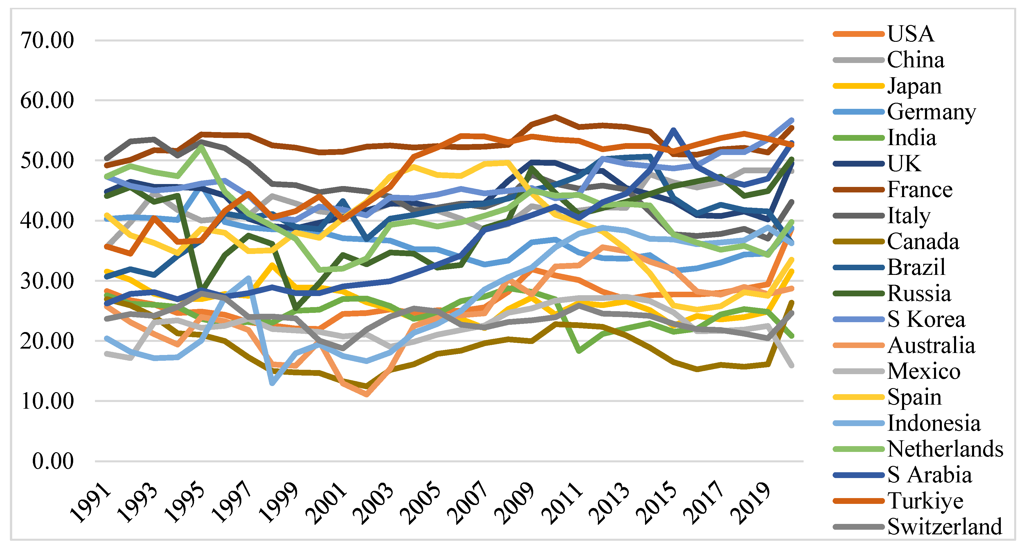
Figure 3. Trends of the G/Y of the countries. Source: drawn by the author.

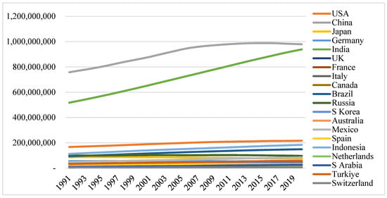
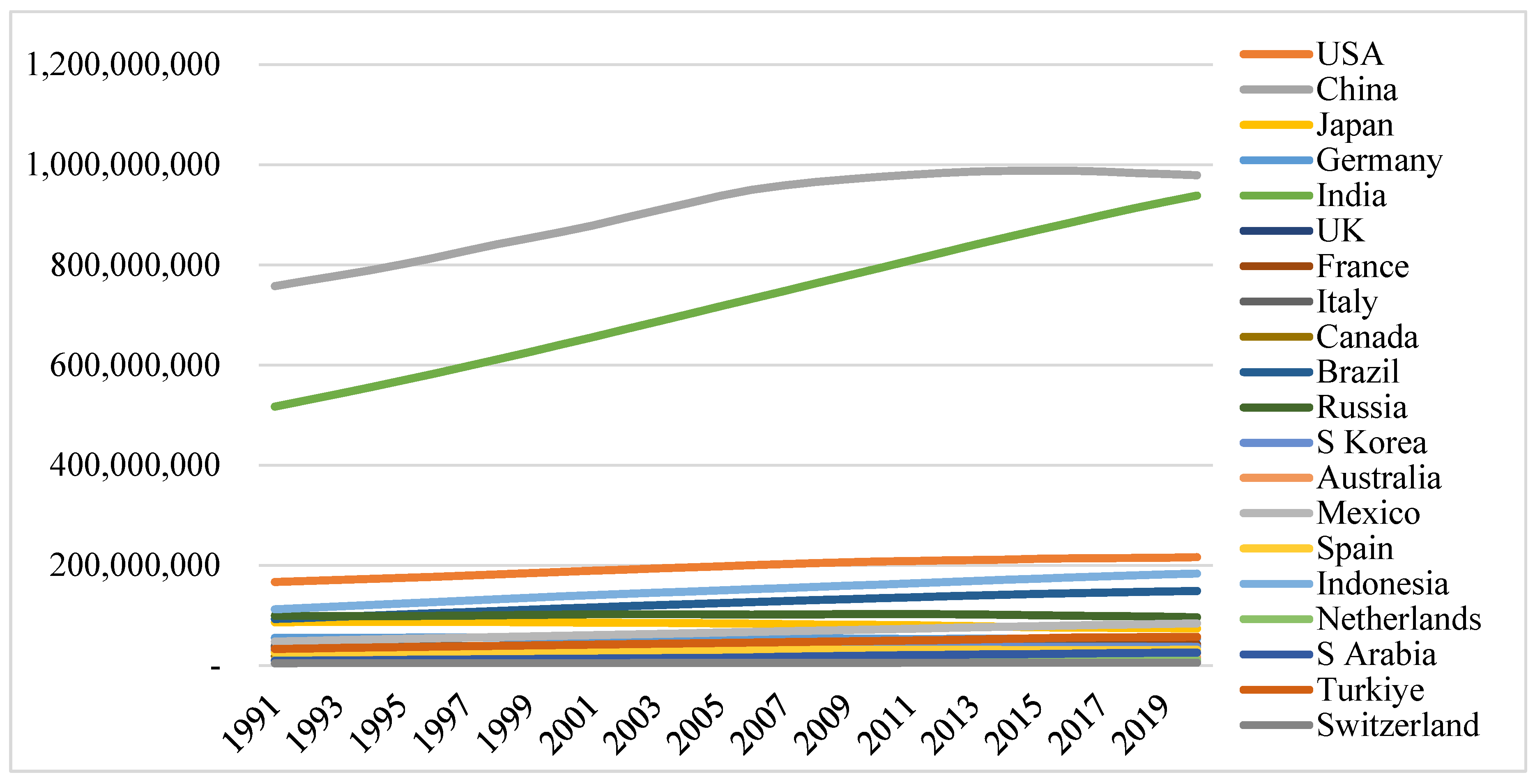
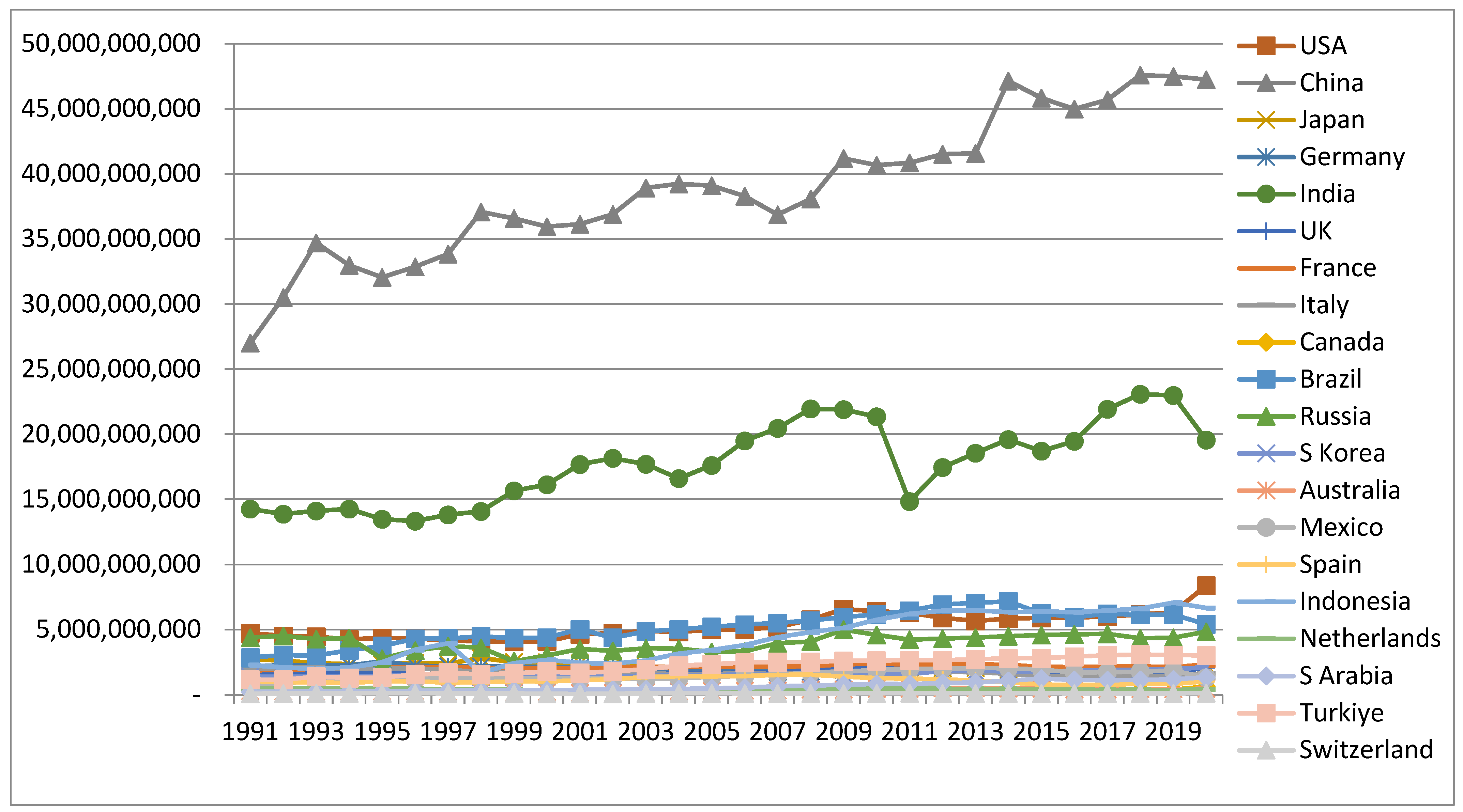
Figure 4. Trends of the total working population of the countries. Source: drawn by the author.

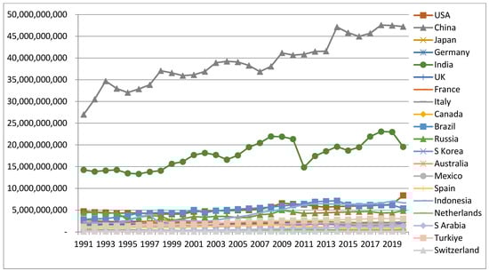
Figure 5. Trends of the interaction effect (G/Y × L) of the countries. Source: drawn by the author.

Figure 3 shows that the governments’ shares in the GDP are relatively higher in the developed countries compared to the developing ones. France and Italy are the front-runners in this respect, and countries like India and Mexico are at the bottom level. The series visually show the presence of unit roots.

It is found from Figure 4 that the population series are maintaining rising trends in the working-age group. China and India are far away from the rest of the selected countries in this respect. The population figures between China and India are going to converge soon. As the working-age population stands for the true labor force, these two countries have the potential for higher economic growth compared to the rest of the world. In the Barro model of growth, population force works as a scale effect (Equation (10)) which may lead to a higher growth of per capita consumption and PCGDP. The series for all look nonstationary again.

Figure 5 depicts the trends in the interaction effect of public share and population which show that the series are rising, with China and India being the front-runners and Switzerland, Turkiye and S. Arabia at the bottom level.

The series again visually show nonstationary features with high magnitudes for the leading countries in the list. The natures of the series are tested in the following section.

4.2. Unit Root Test Results

Since this study has 30 year points and the diagrams of all the indicators show fluctuations, there is a need to test whether there are stochastic properties in the indicators to avoid spurious statistical results. The stochastic properties, or the existence of unit roots, are tested in line with the ADF technique and estimated by Equations (11) and (12).

The results (refer to Table 1) show that all the series suffer from unit root problems in their level values and so they are nonstationary at their levels. But after differencing once for all four series, it is found that 12 out of 20 countries show all of the four series having the I(1) property while the other 8 have the I(2) property in at least one of the indicators.

Table 1. Unit root test results of all the indicators.

	ADF Statistics (Probability)
Country	G/Y Ratio (Level)	Population (Level)	(G/Y) × Population (Level)	PCGDP Growth (Level)	G/Y Ratio (1st Diff.)	Population (1st Diff.)	(G/Y) × Population (1st Diff.)	PCGDP Growth (1st Diff.)
USA	−1.3 (0.50)	−2.2 (0.12)	−2.3 (0.09)	−2.7 (0.07)	−4.3 (0.00) *	−3.2 (0.02) *	−4.1 (0.00) *	−3.7 (0.00) *
China	−1.2 (0.60)	−1.99 (0.15)	−2.57 (0.09)	−1.7 (0.61)	−5.25 (0.00)	−3.0 (0.05) *	−6.57 (0.00)	−7.7 (0.00) *
Japan	−2.1 (0.28)	−1.32 (0.65)	−2.29 (0.30)	−2.6 (0.10)	−5.01 (0.00)	−3.32 (0.05)	−5.29 (0.00)	−3.99 (0.00)
Germany	−2.4 (0.18)	−1.61 (0.41)	−2.13 (0.30)	−2.5 (0.17)	−6.44 (0.00)	−3.61 (0.01)	−6.13 (0.00)	−5.13 (0.00)
India	−2.8 (0.10)	−1.98 (0.35)	−2.75 (0.11)	−2.0 (0.20)	−4.84 (0.00)	−2.98 (0.05)	−4.75 (0.00)	−4.06 (0.00)
UK	−1.9 (0.52)	−1.62 (0.63)	−1.96 (0.52)	−2.6 (0.12)	−3.97 (0.00)	−3.6 (0.00) *	−4.96 (0.00) *	−4.67 (0.00)
France	−2.0 (0.27)	−1.65 (0.63)	−2.40 (0.14)	−2.55 (0.13)	−4.06 (0.00)	−3.65 (0.01)	−3.90 (0.00)	−4.55 (0.00)
Italy	−2.1 (0.22)	−1.98 (0.35)	−2.30 (0.16)	−2.50 (0.14)	−4.15 (0.00)	−2.98 (0.05)	−4.30 (0.00)	−4.50 (0.00)
Canada	−2.1 (0.26)	−1.99 (0.34)	−1.69 (0.38)	−2.75 (0.09)	−4.1 (0.00) *	−3.9 (0.00) *	−3.7 (0.01) *	−5.75 (0.00)
Brazil	−2.2 (0.00)	−1.98 (0.35)	−2.86 (0.07)	−2.60 (0.11)	−5.22 (0.00)	−2.98 (0.05)	−4.86 (0.00)	−3.60 (0.01)
Russia	−2.1 (0.26)	−2.54 (0.16)	−2.15 (0.30)	−2.82 (0.08)	−6.10 (0.00)	−4.5 (0.00) *	−6.15 (0.00)	−3.82 (0.00)
S. Korea	−2.3 (0.25)	−2.40 (0.18)	−2.73 (0.0/)	−2.26 (0.21)	−4.30 (0.00)	−4.4 (0.00) *	−4.73 (0.00)	−5.26 (0.00)
Australia	−2.1 (0.27)	−1.97 (0.35)	−2.00 (0.32)	−2.79 (0.09)	−5.1 (0.00)	−2.97 (0.05)	−5.00 (0.00)	−3.79 (0.00)
Mexico	−1.8 (0.62)	−1.25 (0.83)	−2.01 (0.44)	−2.72 (0.09)	−3.79 (0.00)	−3.2 (0.03) *	−3.01 (0.04)	−4.72 (0.00)
Spain	−2.1 (0.25)	−2.10 (0.24)	−1.99 (0.46)	−2.85 (0.07)	−3.01 (0.05)	−3.10 (0.04)	−2.99 (0.05)	−3.85 (0.00)
Indonesia	−2.8 (0.08)	−2.38 (0.19)	−2.66 (0.09)	−2.73 (0.08)	−5.80 (0.00)	−4.38 (0.00)	−5.66 (0.00)	−3.73 (0.00)
Netherlands	−2.4 (0.18)	−2.21 (0.27)	−2.30 (0.26)	−2.49 (0.14)	−4.34 (0.00)	−3.21 (0.03)	−4.30 (0.00)	−4.49 (0.00)
S. Arabia	−2.9 (0.07)	−2.14 (0.30)	−2.71 (0.07)	−2.42 (0.15)	−4.95 (0.00)	−3.14 (0.04)	−6.71 (0.00) *	−4.42 (0.00)
Turkiye	−2.1 (0.27)	−2.81 (0.07)	−2.62 (0.09)	−2.61 (0.11)	−6.09 (0.00)	−4.81 (0.00)	−5.62 (0.00)	−4.61 (0.00)
Switzerland	−2.4 (0.18)	−1.98 (0.35)	−1.58 (0.41)	−2.73 (0.08)	−4.24 (0.00)	−2.98 (0.05)	−3.58 (0.01)	−4.73 (0.00)

Note: * mark indicates I(2) series. Source: author’s calculations.

4.3. Johansen Cointegration Test Results

As the number of endogenous variables is more than two, we use the VAR model to identify the optimum lag and cointegration among the four variables. The optimum lag is selected by looking at the minimum values of most of the testing criteria such as LR, final prediction error (FPE), Akaike information criterion (AIC), Schwarz information criterion (SIC) and Hannan–Quinn information criterion (HQIC). In all the cases with each of the four indicators playing the role of dependent variable interchangeably, the optimum lag is observed to be 2 (the results are not shown in tables). The Johansen cointegration test technique is used, and the results are presented in Table 2. This test is performed to see whether the lower-order values are cointegrated.

Table 2. Johansen cointegration test results.

Country	Hypothesized No. of CEs	Trace Statistics (Prob)	Remarks
USA *	None *	69.303 (0.00)	The variables are cointegrated and there is 1 cointegrating equation at the 0.05 level
	At most 1 *	23.036 (0.38)
	At most 2	8.0005 (0.13)
	At most 3	2.606 (0.11)
China *	None *	103.4 (0.00)	The variables are cointegrated and there are 4 cointegrating equations at the 0.05 level
	At most 1 *	42.65 (0.00)
	At most 2	19.96 (0.00)
	At most 3	5.39 (0.02)
Japan	None *	54.209 (0.01)	The variables are cointegrated and there is 1 cointegrating equation at the 0.05 level
	At most 1 *	22.017 (0.29)
	At most 2	9.316 (0.33)
	At most 3	2.336 (0.12)
Germany	None *	43.60 (0.11)	No cointegration
	At most 1 *	21.16 (0.34)
	At most 2	7.25 (0.54)
	At most 3	1.53 (0.21)
India	None *	62.52 (0.00)	The variables are cointegrated and there is 1 cointegrating equation at the 0.05 level
	At most 1 *	23.76 (0.21)
	At most 2	11.47 (0.18)
	At most 3	3.04 (0.08)
UK *	None *	49.16 (0.03)	The variables are cointegrated and there is 1 cointegrating equation at the 0.05 level
	At most 1 *	19.57 (0.45)
	At most 2	7.54 (0.51)
	At most 3	2.76 (0.09)
France	None *	80.95 (0.00)	The variables are cointegrated and there are 4 cointegrating equations at the 0.05 level
	At most 1 *	43.05 (0.00)
	At most 2	19.18 (0.01)
	At most 3	5.86 (0.01)
Italy	None *	47.56 (0.00)	The variables are cointegrated and there is 1 cointegrating equation at the 0.05 level
	At most 1 *	28.79 (0.06)
	At most 2	14.88 (0.06)
	At most 3	4.68 (0.06)
Canada *	None *	38.56 (0.22)	No cointegration
	At most 1 *	27.79 (0.11)
	At most 2	13.88 (0.06)
	At most 3	5.68 (0.06)
Brazil	None *	77.33 (0.00)	The variables are cointegrated and there are 2 cointegrating equations at the 0.05 level
	At most 1 *	38.01 (0.00)
	At most 2	9.86 (0.29)
	At most 3	0.28 (0.59)
Russia *	None *	54.36 (0.01)	The variables are cointegrated and there are 2 cointegrating equations at the 0.05 level
	At most 1 *	32.37 (0.02)
	At most 2	13.18 (0.10)
	At most 3	3.76 (0.06)
S. Korea *	None *	70.63 (0.00)	The variables are cointegrated and there are 2 cointegrating equations at the 0.05 level
	At most 1 *	38.50 (0.00)
	At most 2	11.51 (0.18)
	At most 3	0.189 (0.66)
Australia	None *	59.83 (0.00)	The variables are cointegrated and there are 2 cointegrating equations at the 0.05 level
	At most 1 *	19.91 (0.43)
	At most 2	4.33 (0.87)
	At most 3	0.15 (0.70)
Mexico *	None *	98.71 (0.00)	The variables are cointegrated and there are 3 cointegrating equations at the 0.05 level
	At most 1 *	45.36 (0.00)
	At most 2	18.45 (0.01)
	At most 3	1.95 (0.16)
Spain	None *	52.67 (0.00)	The variables are cointegrated and there is 1 cointegrating equation at the 0.05 level
	At most 1 *	23.74 (0.20)
	At most 2	12.92 (0.11)
	At most 3	2.59 (0.09)
Indonesia	None *	68.93 (0.00)	The variables are cointegrated and there are 2 cointegrating equations at the 0.05 level
	At most 1 *	31.05 (0.03)
	At most 2	5.60 (0.74)
	At most 3	3.15 (0.08)
Netherlands	None *	47.99 (0.04)	The variables are cointegrated and there is 1 cointegrating equation at the 0.05 level
	At most 1 *	21.95 (0.29)
	At most 2	11.25 (0.19)
	At most 3	3.45 (0.06)
S. Arabia *	None *	56.16 (0.00)	The variables are cointegrated and there are 4 cointegrating equations at the 0.05 level
	At most 1 *	29.67 (0.01)
	At most 2	15.47 (0.05)
	At most 3	5.45 (0.01)
Turkiye	None *	55.75 (0.00)	The variables are cointegrated and there is 1 cointegrating equation at the 0.05 level
	At most 1 *	28.17 (0.07)
	At most 2	10.89 (0.27)
	At most 3	4.56 (0.03)
Switzerland	None *	78.83 (0.00)	The variables are cointegrated and there is 1 cointegrating equation at the 0.05 level
	At most 1 *	28.87 (0.31)
	At most 2	13.56 (0.10)
	At most 3	0.009 (0.94)

Note: * marks in the first column indicate the series of the countries following the I(2) feature. Again, * marks in the second column denote rejection of the ‘no cointegration’ hypothesis at the 0.05 level. Source: author’s calculations.

It is observed from the table that the Trace Statistics show cointegration results among the variables in 18 countries at the 0.05 level of significance, but this was not shown for Germany and Canada. This means the four growth indicators as per the Barro model are cointegrated and there are long-run relationships among them. This is a valid justification for whether the government sector in terms of good institutions has good impacts on per capita income growth. The leading countries in the world in terms of GDP have experienced higher growth of outputs due to their strong public institutions, their labor force and the coordination between public spending and labor force.

Now, we test for short-run dynamics among the four variables around the equilibrium relations by VECM to see whether the cointegrating relations are stable. Further, VECM analysis is performed for those countries that have long-run relations among the variables. The results of VECM are given in Table 3.

Table 3. Long-run causality test results through VECM.

Country	Dependent Variables	Independent Variables	EC Term(η)	Prob.	Remarks
China	G/Y	G/Y × L, Population, PCGDP	15.59	0.00	No LR causality
	G/Y × L	G/Y, Population, PCGDP	0.0001	0.00	No LR causality
	Population	G/Y, G/Y × L, PCGDP	−271,179	0.31	No LR causality
	PCGDP Growth	G/Y, G/Y × L, Population	579.21	0.26	No LR causality
Japan	G/Y	G/Y × L, Population, PCGDP	−23.59	0.02	G/Y × L, Population, PCGDP→G/Y
	G/Y × L	G/Y, Population, PCGDP	−2.0000	0.02	G/Y, Population, PCGDP→G/Y × L
	Population	G/Y, G/Y × L, PCGDP	401,023	0.39	No LR causality
	PCGDP Growth	G/Y, G/Y × L, Population	37,322	0.00	No LR causality
India	G/Y	G/Y × L, Population, PCGDP	2.003	0.14	No LR causality
	G/Y × L	G/Y, Population, PCGDP	1,790,000	0.09	No LR causality
	Population	G/Y, G/Y × L, PCGDP	−294,086	0.01	G/Y, G/Y × L, PCGDP→ Population
	PCGDP Growth	G/Y, G/Y × L, Population	61.67	0.22	No LR causality
UK	G/Y	G/Y × L, Population, PCGDP	−0.063	0.98	No LR causality
	G/Y × L	G/Y, Population, PCGDP	4,112,746	0.97	No LR causality
	Population	G/Y, G/Y × L, PCGDP	79,800	0.00	No LR causality
	PCGDP Growth	G/Y, G/Y × L, Population	−2353	0.46	No LR causality
France	G/Y	G/Y × L, Population, PCGDP	−1.02	0.19	No LR causality
	G/Y × L	G/Y, Population, PCGDP	−39,756,754	0.22	No LR causality
	Population	G/Y, G/Y × L, PCGDP	39,862	0.00	No LR causality
	PCGDP Growth	G/Y, G/Y × L, Population	−1219	0.31	No LR causality
Brazil	G/Y	G/Y × L, Population, PCGDP	0.07	0.03	No LR causality
	G/Y × L	G/Y, Population, PCGDP	9,181,923	0.03	No LR causality
	Population	G/Y, G/Y × L, PCGDP	−338.3	0.26	No LR causality
	PCGDP Growth	G/Y, G/Y × L, Population	−26.16	0.18	No LR causality
Russia	G/Y	G/Y × L, Population, PCGDP	−23.42	0.00	G/Y × L, Population, PCGDP→G/Y
	G/Y × L	G/Y, Population, PCGDP	−23,500,000	0.00	G/Y, Population, PCGDP→G/Y × L
	Population	G/Y, G/Y × L, PCGDP	−233,665	0.05	G/Y, G/Y × L, PCGDP→ Population
	PCGDP Growth	G/Y, G/Y × L, Population	3318	0.13	No LR causality
S. Korea	G/Y	G/Y × L, Population, PCGDP	−14.58	0.03	G/Y × L, Population, PCGDP→G/Y
	G/Y × L	G/Y, Population, PCGDP	−5,040,000	0.03	G/Y, Population, PCGDP→G/Y × L
	Population	G/Y, G/Y × L, PCGDP	−64,407	0.70	No LR causality
	PCGDP Growth	G/Y, G/Y × L, Population	−23.39	0.00	G/Y, G/Y × L, Population→ PCGDP
Australia	G/Y	G/Y×L, Population, PCGDP	−0.31	0.03	No LR causality
	G/Y × L	G/Y, Population, PCGDP	−2,040,000	0.13	No LR causality
	Population	G/Y, G/Y × L, PCGDP	−64,407	0.70	No LR causality
	PCGDP Growth	G/Y, G/Y × L, Population	0.49	0.01	No LR causality
Mexico	G/Y	G/Y × L, Population, PCGDP	4.77	0.08	No LR causality
	G/Y × L	G/Y, Population, PCGDP	45,600,000	0.03	No LR causality
	Population	G/Y, G/Y × L, PCGDP	−14,147	0.74	No LR causality
	PCGDP Growth	G/Y, G/Y × L, Population	8.89	0.04	No LR causality
Spain	G/Y	G/Y × L, Population, PCGDP	6.085	0.00	G/Y × L, Population, PCGDP→G/Y
	G/Y × L	G/Y, Population, PCGDP	−17,000,000	0.00	G/Y, Population, PCGDP→G/Y × L
	Population	G/Y, G/Y × L, PCGDP	99,605	0.41	No LR causality
	PCGDP Growth	G/Y, G/Y × L, Population	6.475	0.00	No LR causality
Indonesia	G/Y	G/Y × L, Population, PCGDP	−2.76	0.33	No LR causality
	G/Y × L	G/Y, Population, PCGDP	−30,900,000	0.41	No LR causality
	Population	G/Y, G/Y × L, PCGDP	79,385	0.00	No LR causality
	PCGDP Growth	G/Y, G/Y × L, Population	−0.91	0.05	G/Y, G/Y × L, Population→ PCGDP
Netherlands	G/Y	G/Y × L, Population, PCGDP	3.62	0.55	No LR causality
	G/Y × L	G/Y, Population, PCGDP	41,572,903	0.52	No LR causality
	Population	G/Y, G/Y × L, PCGDP	39,787	0.00	No LR causality
	PCGDP Growth	G/Y, G/Y × L, Population	−0.87	0.77	No LR causality
S. Arabia	G/Y	G/Y × L, Population, PCGDP	−4.24	0.00	G/Y × L, Population, PCGDP→G/Y
	G/Y × L	G/Y, Population, PCGDP	−87,856,447	0.00	G/Y, Population, PCGDP→G/Y × L
	Population	G/Y, G/Y × L, PCGDP	45,042	0.47	No LR causality
	PCGDP Growth	G/Y, G/Y × L, Population	0.14	0.00	No LR causality
Turkiye	G/Y	G/Y × L, Population, PCGDP	−1.44	0.00	G/Y × L, Population, PCGDP→G/Y
	G/Y × L	G/Y, Population, PCGDP	−53,429,008	0.01	G/Y, Population, PCGDP→G/Y × L
	Population	G/Y, G/Y × L, PCGDP	32,999	0.03	No LR causality
	PCGDP Growth	G/Y, G/Y × L, Population	−0.46	0.41	No LR causality
Switzerland	G/Y	G/Y × L, Population, PCGDP	−0.936	0.12	No LR causality
	G/Y × L	G/Y, Population, PCGDP	−4,546,936	0.16	No LR causality
	Population	G/Y, G/Y × L, PCGDP	−1776	0.36	No LR causality
	PCGDP Growth	G/Y, G/Y × L, Population	−9.91	0.01	G/Y, G/Y × L, Population→PCGDP

Note: PCGDP in columns 3 and 6 represents the growth of PCGDP. Source: author’s own calculations.

It is observed that the errors in maximum of the models are not corrected as the signs of the error correction terms are not negative and significant. Though there are some negative values of the said term, they are not statistically significant in most of the cases. Only in the case of three countries, S. Korea, Indonesia and Switzerland, are there significant error corrections when PCGDP Growth is the endogenous dependent variable. It can also be said that good public institutions, population and their interaction terms affect or rather have a causal influence on the per capita GDP growth rate in the long run. On the other hand, PCGDP Growth, population and the interaction term have a causal influence on the government share of GDP in the long run in the case of some countries such as Japan, Russia, S. Korea, Spain, S. Arabia and Turkiye. Again, population is influenced by the rest of the factors in the long run in the case of India and Russia. This study does not find any error correction or long-run causality in any of the four combinations of the variables in the case of China, the UK, France, Italy, Brazil, Australia, Mexico and the Netherlands.

4.4. Short-Run Causality Test Results

Although there are absences in the long-run causal relations in most of the countries, at least for the occasions where PCGDP Growth is held as an endogenous dependent variable, there may be the possibilities of short-run causal interplays among the variables. The Wald test is used to test for short-run causality among the variables. The results are given in Table 4. The decision rule is through the values of Chi-Square test statistics with probabilities less than 0.05.

Table 4. Short-run causality test results (Wald test).

Country	Dependent Variables	Independent Variables	Chi-Square Value	Prob.	Remarks
USA	G/Y	G/Y × L, Population, PCGDP	2.468	0.480	No SR causality
	G/Y × L	G/Y, Population, PCGDP	7.768	0.051	G/Y, Population, PCGDP→G/Y × L
	Population	G/Y, G/Y × L, PCGDP	3.722	0.293	No SR causality
	PCGDP Growth	G/Y, G/Y × L, Population	4.035	0.257	No SR causality
China	G/Y	G/Y × L, Population, PCGDP	17.95	0.00	G/Y × L, Population, PCGDP→G/Y
	G/Y × L	G/Y, Population, PCGDP	19.66	0.00	G/Y, Population, PCGDP→G/Y × L
	Population	G/Y, G/Y × L, PCGDP	3.15	0.78	No SR causality
	PCGDP Growth	G/Y, G/Y × L, Population	6.38	0.38	No SR causality
Japan	G/Y	G/Y × L, Population, PCGDP	5.28	0.50	No SR causality
	G/Y × L	G/Y, Population, PCGDP	6.078	0.41	No SR causality
	Population	G/Y, G/Y × L, PCGDP	2.27	0.89	No SR causality
	PCGDP Growth	G/Y, G/Y × L, Population	19.53	0.003	G/Y, G/Y × L, Population→ PCGDP
Germany	G/Y	G/Y × L, Population, PCGDP	1.38	0.96	No SR causality
	G/Y × L	G/Y, Population, PCGDP	1.53	0.95	No SR causality
	Population	G/Y, G/Y × L, PCGDP	19.60	0.00	G/Y, G/Y × L, PCGDP→ Population
	PCGDP Growth	G/Y, G/Y × L, Population	1.55	0.00	No SR causality
India	G/Y	G/Y × L, Population, PCGDP	6.48	0.37	No SR causality
	G/Y × L	G/Y, Population, PCGDP	7.64	0.26	No SR causality
	Population	G/Y, G/Y × L, PCGDP	13.06	0.04	G/Y, G/Y × L, PCGDP→ Population
	PCGDP Growth	G/Y, G/Y × L, Population	3.40	0.75	No SR causality
UK	G/Y	G/Y × L, Population, PCGDP	4.25	0.64	No SR causality
	G/Y × L	G/Y, Population, PCGDP	4.27	0.63	No SR causality
	Population	G/Y, G/Y × L, PCGDP	16.11	0.01	G/Y, G/Y × L, PCGDP→Population
	PCGDP Growth	G/Y, G/Y × L, Population	15.81	0.05	G/Y, G/Y × L, Population→PCGDP
France	G/Y	G/Y × L, Population, PCGDP	3.11	0.79	No SR causality
	G/Y × L	G/Y, Population, PCGDP	3.95	0.68	No SR causality
	Population	G/Y, G/Y × L, PCGDP	50.40	0.00	G/Y, G/Y × L, PCGDP→Population
	PCGDP Growth	G/Y, G/Y × L, Population	3.25	0.77	G/Y, G/Y × L, Population→PCGDP
Italy	G/Y	G/Y × L, Population, PCGDP	13.06	0.04	G/Y × L, Population, PCGDP→G/Y
	G/Y × L	G/Y, Population, PCGDP	12.58	0.05	G/Y, Population, PCGDP→G/Y × L
	Population	G/Y, G/Y × L, PCGDP	3.09	0.79	No SR causality
	PCGDP Growth	G/Y, G/Y × L, Population	3.12	0.79	No SR causality
Canada	G/Y	G/Y × L, Population, PCGDP	6.27	0.39	No SR causality
	G/Y × L	G/Y, Population, PCGDP	6.29	0.39	No SR causality
	Population	G/Y, G/Y × L, PCGDP	1.34	0.96	No SR causality
	PCGDP Growth	G/Y, G/Y × L, Population	8.70	0.19	No SR causality
Brazil	G/Y	G/Y × L, Population, PCGDP	27.10	0.00	G/Y × L, Population, PCGDP→G/Y
	G/Y × L	G/Y, Population, PCGDP	28.22	0.00	G/Y, Population, PCGDP→G/Y × L
	Population	G/Y, G/Y × L, PCGDP	17.08	0.00	G/Y, G/Y × L, PCGDP→ Population
	PCGDP Growth	G/Y, G/Y × L, Population	12.30	0.05	G/Y, G/Y × L, Population→PCGDP
Russia	G/Y	G/Y × L, Population, PCGDP	9.30	0.15	No SR causality
	G/Y × L	G/Y, Population, PCGDP	9.03	0.17	No SR causality
	Population	G/Y, G/Y × L, PCGDP	19.87	0.00	G/Y, G/Y × L, PCGDP→Population
	PCGDP Growth	G/Y, G/Y × L, Population	6.68	0.35	G/Y, G/Y × L, Population→PCGDP
S. Korea	G/Y	G/Y × L, Population, PCGDP	6.94	0.32	No SR causality
	G/Y × L	G/Y, Population, PCGDP	7.41	0.28	No SR causality
	Population	G/Y, G/Y × L, PCGDP	26.41	0.00	G/Y, G/Y × L, PCGDP→Population
	PCGDP Growth	G/Y, G/Y × L, Population	27.99	0.00	G/Y, G/Y × L, Population→PCGDP
Australia	G/Y	G/Y × L, Population, PCGDP	4.62	0.59	No SR causality
	G/Y × L	G/Y, Population, PCGDP	6.62	0.35	No SR causality
	Population	G/Y, G/Y × L, PCGDP	4.12	0.66	No SR causality
	PCGDP Growth	G/Y, G/Y × L, Population	18.59	0.00	G/Y, G/Y × L, Population→PCGDP
Mexico	G/Y	G/Y × L, Population, PCGDP	10.12	0.12	No SR causality
	G/Y × L	G/Y, Population, PCGDP	11.56	0.07	No SR causality
	Population	G/Y, G/Y × L, PCGDP	18.86	0.00	G/Y, G/Y × L, PCGDP→Population
	PCGDP Growth	G/Y, G/Y × L, Population	25.025	0.00	G/Y, G/Y × L, Population→PCGDP
Spain	G/Y	G/Y × L, Population, PCGDP	51.77	0.00	G/Y × L, Population, PCGDP→G/Y
	G/Y × L	G/Y, Population, PCGDP	44.47	0.00	G/Y, Population, PCGDP→G/Y × L
	Population	G/Y, G/Y × L, PCGDP	2.51	0.86	No SR causality
	PCGDP Growth	G/Y, G/Y × L, Population	22.86	0.00	G/Y, G/Y × L, Population→PCGDP
Indonesia	G/Y	G/Y × L, Population, PCGDP	7.85	0.24	No SR causality
	G/Y × L	G/Y, Population, PCGDP	8.75	0.19	No SR causality
	Population	G/Y, G/Y × L, PCGDP	15.67	0.01	G/Y, G/Y × L, PCGDP→Population
	PCGDP Growth	G/Y, G/Y × L, Population	32.92	0.00	G/Y, G/Y × L, Population→PCGDP
Netherlands	G/Y	G/Y × L, Population, PCGDP	1.07	0.98	No SR causality
	G/Y × L	G/Y, Population, PCGDP	1.09	0.98	No SR causality
	Population	G/Y, G/Y × L, PCGDP	13.19	0.05	G/Y, G/Y × L, PCGDP→Population
	PCGDP Growth	G/Y, G/Y × L, Population	0.82	0.99	No SR causality
S. Arabia	G/Y	G/Y × L, Population, PCGDP	19.52	0.00	G/Y × L, Population, PCGDP→G/Y
	G/Y × L	G/Y, Population, PCGDP	15.75	0.01	G/Y, Population, PCGDP→G/Y × L
	Population	G/Y, G/Y × L, PCGDP	2.84	0.83	No SR causality
	PCGDP Growth	G/Y, G/Y × L, Population	7.77	0.25	No SR causality
Turkiye	G/Y	G/Y × L, Population, PCGDP	12.98	0.05	G/Y × L, Population, PCGDP→G/Y
	G/Y × L	G/Y, Population, PCGDP	12.65	0.05	G/Y, Population, PCGDP→G/Y × L
	Population	G/Y, G/Y × L, PCGDP	6.56	0.36	No SR causality
	PCGDP Growth	G/Y, G/Y × L, Population	5.82	0.44	No SR causality
Switzerland	G/Y	G/Y × L, Population, PCGDP	5.44	0.48	No SR causality
	G/Y × L	G/Y, Population, PCGDP	4.95	0.54	No SR causality
	Population	G/Y, G/Y × L, PCGDP	23.66	0.00	G/Y, G/Y × L, PCGDP→Population
	PCGDP Growth	G/Y, G/Y × L, Population	34.26	0.00	G/Y, G/Y × L, Population→PCGDP

Note: PCGDP in columns 3 and 6 represents the growth of PCGDP. Source: author’s own calculations.

In 11 countries on the list, public institutions associated with population and the interaction term have a causal influence on the growth of PCGDP. These countries are Japan, the UK, France, Brazil, Russia, S. Korea, Australia, Mexico, Spain, Indonesia and Switzerland. Thus, in most of the countries, the growth of PCGDP is explained by good public participation coupled with its impacts on the population. In other words, the Barro model of endogenous growth incorporating public institutions works well in the world’s leading countries in terms of the gross domestic product. It is also observed that the growth of income and population have a causal influence on government participation in countries like China, Italy, Brazil, Spain, S. Arabia and Turkiye. On the other hand, the interaction factor is influenced by income growth, labor force and government participation in the countries such as the USA, China, Italy, Brazil, Spain, S. Arabia and Turkiye. There are common results in the case of G/Y and G/Y × L for the above sets of countries. Brazil is the only country in the list where all four occasions of causal interplays have worked. Canada is the only country in the list where no causal interplays among the four associated variables are observed.

4.5. Robustness of the Results

To check the robustness of the results of the model, this study tests for the normality of the residuals. Table 5 presents the results of the different models specified against the criteria of serial autocorrelation, heteroskedasticity and normality checks of the residuals through the Breusch–Godfrey Serial Correlation LM Test, Breusch–Pagan–Godfrey Heteroskedasticity Test and Histogram-Normality Test, respectively.

Table 5. Residuals’ diagnostic checking (only probabilities are noted).

Country	Dependent Variables	Breusch–Godfrey Serial Correlation LM Test	Breusch–Pagan–Godfrey Heteroskedasticity Test	Histogram-Normality Test	Remarks
China	G/Y	0.999	0.853	0.934	Model has good fit as the errors satisfy all the diagnostic checking
	G/Y × L	0.999	0.838	0.22	Model has partially good fit as the errors do not satisfy the normality property
	Population	0.999	0.98	0.037	Model has partially good fit as the errors do not satisfy the normality property
	PCGDP Growth	0.995	0.70	0.72	Model has good fit as the errors satisfy all the diagnostic checking
Japan	G/Y	0.992	0.36	0.95	Model has good fit as the errors satisfy all the diagnostic checking
	G/Y × L	0.995	0.27	0.96	Model has good fit as the errors satisfy all the diagnostic checking
	Population	0.99	0.54	0.21	Model has partially good fit as the errors do not satisfy the normality property
	PCGDP Growth	0.99	0.70	0.60	Model has good fit as the errors satisfy all the diagnostic checking
India	G/Y	0.20	0.93	0.65	Model has good fit as the errors satisfy all the diagnostic checking
	G/Y × L	0.99	0.59	0.005	Model has partially good fit as the errors do not satisfy the normality property
	Population	0.89	0.32	0.48	Model has good fit as the errors satisfy all the diagnostic checking
	PCGDP Growth	0.98	0.12	0.96	Model has good fit as the errors satisfy all the diagnostic checking
UK	G/Y	0.96	0.40	0.50	Model has good fit as the errors satisfy all the diagnostic checking
	G/Y × L	0.99	0.65	0.83	Model has good fit as the errors satisfy all the diagnostic checking
	Population	0.58	0.30	0.54	Model has good fit as the errors satisfy all the diagnostic checking
	PCGDP Growth	0.99	0.12	0.96	Model has good fit as the errors satisfy all the diagnostic checking
France	G/Y	0.98	0.54	0.60	Model has good fit as the errors satisfy all the diagnostic checking
	G/Y × L	0.85	0.64	0.72	Model has good fit as the errors satisfy all the diagnostic checking
	Population	0.78	0.88	0.69	Model has good fit as the errors satisfy all the diagnostic checking
	PCGDP Growth	0.84	0.91	0.84	Model has good fit as the errors satisfy all the diagnostic checking
Brazil	G/Y	0.99	0.88	0.81	Model has good fit as the errors satisfy all the diagnostic checking
	G/Y × L	0.85	0.78	0.68	Model has good fit as the errors satisfy all the diagnostic checking
	Population	0.97	0.83	0.59	Model has good fit as the errors satisfy all the diagnostic checking
	PCGDP Growth	0.85	0.78	0.68	Model has good fit as the errors satisfy all the diagnostic checking
Russia	G/Y	0.99	0.47	0.41	Model has good fit as the errors satisfy all the diagnostic checking
	G/Y × L	0.94	0.58	0.56	Model has good fit as the errors satisfy all the diagnostic checking
	Population	0.88	0.66	0.60	Model has good fit as the errors satisfy all the diagnostic checking
	PCGDP Growth	0.91	0.63	0.55	Model has good fit as the errors satisfy all the diagnostic checking
S. Korea	G/Y	0.97	0.26	0.72	Model has partially good fit as the errors do not satisfy the normality property
	G/Y × L	0.92	0.48	0.77	Model has good fit as the errors satisfy all the diagnostic checking
	Population	0.95	0.65	0.66	Model has good fit as the errors satisfy all the diagnostic checking
	PCGDP Growth	0.94	0.71	0.58	Model has good fit as the errors satisfy all the diagnostic checking
Australia	G/Y	0.99	0.80	0.14	Model has partially good fit as the errors do not satisfy the normality property
	G/Y × L	0.98	0.85	0.45	Model has good fit as the errors satisfy all the diagnostic checking
	Population	0.96	0.86	0.58	Model has good fit as the errors satisfy all the diagnostic checking
	PCGDP Growth	0.97	0.91	0.68	Model has good fit as the errors satisfy all the diagnostic checking
Mexico	G/Y	0.99	0.57	0.19	Model has partially good fit as the errors do not satisfy the normality property
	G/Y × L	0.88	0.61	0.43	Model has good fit as the errors satisfy all the diagnostic checking
	Population	0.95	0.64	0.54	Model has good fit as the errors satisfy all the diagnostic checking
	PCGDP Growth	0.96	0.75	0.62	Model has good fit as the errors satisfy all the diagnostic checking
Spain	G/Y	0.99	0.51	0.007	Model has partially good fit as the errors do not satisfy the normality property
	G/Y × L	0.99	0.60	0.78	Model has good fit as the errors satisfy all the diagnostic checking
	Population	0.98	0.62	0.71	Model has good fit as the errors satisfy all the diagnostic checking
	PCGDP Growth	0.97	0.71	0.65	Model has good fit as the errors satisfy all the diagnostic checking
Indonesia	G/Y	0.91	0.69	0.66	Model has good fit as the errors satisfy all the diagnostic checking
	G/Y × L	0.97	0.72	0.68	Model has good fit as the errors satisfy all the diagnostic checking
	Population	0.95	0.75	0.78	Model has good fit as the errors satisfy all the diagnostic checking
	PCGDP Growth	0.98	0.82	0.58	Model has good fit as the errors satisfy all the diagnostic checking
Netherlands	G/Y	0.99	0.72	0.012	Model has partially good fit as the errors do not satisfy the normality property
	G/Y × L	0.96	0.81	0.002	Model has partially good fit as the errors do not satisfy the normality property
	Population	0.98	0.77	0.15	Model has partially good fit as the errors do not satisfy the normality property
	PCGDP Growth	0.99	0.68	0.22	Model has partially good fit as the errors do not satisfy the normality property
S. Arabia	G/Y	0.99	0.87	0.42	Model has good fit as the errors satisfy all the diagnostic checking
	G/Y × L	0.98	0.78	0.56	Model has good fit as the errors satisfy all the diagnostic checking
	Population	0.95	0.88	0.62	Model has good fit as the errors satisfy all the diagnostic checking
	PCGDP Growth	0.98	0.74	0.57	Model has good fit as the errors satisfy all the diagnostic checking
Turkiye	G/Y	0.99	0.80	0.51	Model has good fit as the errors satisfy all the diagnostic checking
	G/Y × L	0.98	0.74	0.59	Model has good fit as the errors satisfy all the diagnostic checking
	Population	0.95	0.75	0.65	Model has good fit as the errors satisfy all the diagnostic checking
	PCGDP Growth	0.96	0.81	0.71	Model has good fit as the errors satisfy all the diagnostic checking
Switzerland	G/Y	0.97	0.45	0.01	Model has partially good fit as the errors do not satisfy the normality property
	G/Y × L	0.98	0.66	0.62	Model has good fit as the errors satisfy all the diagnostic checking
	Population	0.99	0.85	0.71	Model has good fit as the errors satisfy all the diagnostic checking
	PCGDP Growth	0.88	0.71	0.56	Model has good fit as the errors satisfy all the diagnostic checking

Note: PCGDP in columns 3 and 6 represents the growth of PCGDP. Source: author’s own calculations.

The validity of having the cointegrating relations for the 18 countries except Canada and Germany is tested for robustness checking.

The results of the table show that they are robust in most of the countries, which enables us to accept the results of cointegration, error correction and causal interplay among the noted indicators.

4.6. Discussion

Comparing the long-run and short-run causality results in reference to Table 2, Table 3 and Table 4, it is said that there are cointegration results among the variables in 18 countries at the 0.05 level of significance. This means that the four growth indicators as per the Barro model are cointegrated and there are long-run relationships among them. This is a valid justification for whether the government sector in terms of good institutions has good impacts on per capita income growth. The results are obtained through the channels where expansion in the public sector leads to expansion in the private sector which satisfies the crowding-in effects. The derived results from the cointegration analysis thus support the forward linkage effects in the first stage and backward linkage in the second stage. The leading countries in the world in terms of GDP have experienced higher growth of outputs due to their strong public institutions, their labor force and the coordination between public spending and labor force. Further, long-run and short-run influences of all three on PCGDP Growth have happened for three countries, namely S. Korea, Indonesia and Switzerland. India is the only country where the case for employment produces similar causality results. No other countries’ results produce any such similar results in long-run and short-run causality. The logic behind the effects of G/Y on population or the reverse is that a good public institution leads to good-quality public institutional outputs in terms of good educational attainment, health benefits (Lucas, 1988), legal and judicial supports, internal and external security (Barro, 1990, 1991), etc., increasing the good-quality population size. On the other hand, for countries having good-quality public institutions, the increase in the population size of these countries will be able to absorb the good public institutional frameworks that will push up their productivity which will then help in increasing growth of per capita consumption and income. The econometric results go in line with the networking as presented in Figure 1. Hence, strengthening public institutional quality through more budgetary allocations and good governance mechanisms might help in increasing private sector investments which combinedly act through the forward linkage as well as backward linkage effects to reap economic benefits in terms of per capita income growth as well as consumption growth of the countries from all groups of economies which may ultimately lead to sustainable development through the attainments of SDGs 8, 9, 12 and 16. The active participation of the governments of countries through stimulus packages during the COVID-19 phase has proved that good institutions always make contributions in recovering countries from economic slowdowns and thus helping in promoting their growths of aggregate as well as per capita incomes.

The empirical evidence thus supports Grossman (1990), Barro (1991), Ghali (1998), Loizides and Vamvoukas (2005), Bhanumurthy et al. (2016), Pahlevi (2017), Chiou-Wei et al. (2010), Das and Mukherjee (2019), Ramirez (1998), Erden and Holcombe (2006), Afonso and St. Aubyn (2008), Grossman (1990), Ghali (1998), Loizides and Vamvoukas (2005), etc., in the cases where it is revealed that the government sizes are the cause of economic growth. On the other hand, it supports studies such as those of Gwartney et al. (1998), Folster and Henrekson (2001), etc., for the instances where it is revealed that the effect of the government size on economic growth is different, or has no long-run or short-run linkages. Further, studies such as those of Barrett and Graddy (2000), Glass and Newig (2019) and Meng (2024) justify the role of the public sector in sustainable development. Thus, the governments of countries in general should spend a significant proportion of their revenues on economic participation in terms of building good institutions to help the private sector excel and lead to further growth in the per capita GDP to reduce poverty and inequality and to act as shock absorbers during the crisis periods. Long-term public sector participation coupled with private sector participation and working population engagements could enhance per capita income and consumption and reduce poverty, which would ensure the sustainability of income generation processes.

5. Concluding Observations

With the objective of examining long-run and short-run linkages among public spending, working population and the interaction terms (between government participation rate and working population) with per capita GDP growth, this study observes that the selected variables in 18 countries, not including Germany and Canada, significantly maintain long-run relations for this study period. On the other hand, in the short run, there are instances in 11 countries of the list where public institutions associated with population and the interaction term have a causal influence on the growth of PCGDP. This means the four growth indicators as per the modified Barro model are cointegrated and there are long-run relationships among them. This is a valid justification for whether the government sector in terms of good institutions has good impacts on per capita income growth and sustainable development. The crucial channels through which the countries have experienced the cointegrating results are the forward and backward linkage effects leading to the crowding-in effects. The countries gained from the combinations of the public and private capital formations as well as the combinations between government participation and working population. Population is, thus, not a growth-retarding factor in the endogenous growth model. The leading countries in the world in terms of GDP are found to have experienced higher growth of outputs due to their strong public institutions, their labor force and the coordination between public spending and labor force.

Although this study has good and acceptable results in terms of the impact of the public institutions, it suffers from some limitations. The inter-country inherent coordinations in the selected indicators are not captured. A panel data model can resolve this issue. This study thus aims to investigate similar relations for a panel of the top twenty countries.

References

- Afonso, A., & Furceri, D. (2010). Government size, composition, volatility, and economic growth. European Journal of Political Economics, 26(4), 517–532. [Google Scholar] [CrossRef]
- Afonso, A., & Jalles, J. (2011). Economic performance and government size. Working paper series, no. 1399. European Central Bank. [Google Scholar]
- Afonso, A., & Jalles, J. T. (2014). Fiscal composition and long-term growth. Applied Economics, 46(3), 349–358. [Google Scholar] [CrossRef]
- Afonso, A., & St. Aubyn, M. (2008). Macroeconomic rates of return of public and private investment crowding-in and crowding-out effects. Working paper series no 864/February. European Central Bank. Available online: www.ecb.europa.eu/pub/pdf/scpwps/ecbwp864.pdf?2888e44ac756b0d892c32a6d3bd05f83 (accessed on 13 August 2024).
- Aschauer, D. (1989). Is public expenditure productive? Journal of Monetary Economics, 23(2), 177–200. [Google Scholar] [CrossRef]
- Barrett, S., & Graddy, K. (2000). Freedom, growth, and the environment. Environment and Development Economics, 5(4), 433–456. [Google Scholar] [CrossRef]
- Barro, R. J. (1989). Economic growth in a cross section of countries. Working paper no. 3120. NBER. [Google Scholar]
- Barro, R. J. (1990). Government spending in a simple model of endogenous growth. Journal of Political Economy, 98(S5), 103–125. [Google Scholar] [CrossRef]
- Barro, R. J. (1991). Economic growth in a cross section of countries. Quarterly Journal of Economics, 106(2), 407–443. [Google Scholar] [CrossRef]
- Barro, R. J. (2001). Human capital and growth. American Economic Review, 91, 12–17. [Google Scholar] [CrossRef]
- Barro, R. J., & Lee, J. W. (1993). International comparisons of educational attainment. Journal of Monetary Economics, 32, 363–394. [Google Scholar] [CrossRef]
- Barro, R. J., & Lee, J. W. (2001). International data on educational attainment: Updates and implications. Oxford Economic Papers, 53, 541–563. [Google Scholar] [CrossRef]
- Barth, J. R., & Bradley, M. D. (1987). The impact of government spending on economic activity. George Washington University. [Google Scholar]
- Ben Zeev, N., Ramey, V. A., & Zubairy, S. (2023). Do government spending multipliers depend on the sign of the shock? AEA Papers and Proceedings, 113, 382–387. [Google Scholar] [CrossRef]
- Bhanumurthy, N., Prasad, M., & Jain, R. (2016). Public expenditure, governance and human development: A case of Madhya Pradesh. Available online: http://www.nipfp.org.in/publications/working-papers/1760/ (accessed on 15 August 2024).
- Blankenau, W. F., & Simpson, N. B. (2004). Public education expenditures and growth. Journal of Development Economics, 73(2), 583–605. [Google Scholar] [CrossRef]
- Bolton, M. (2021). Public sector understanding of sustainable development and the sustainable development goals: A case study of Victoria, Australia. Current Research in Environmental Sustainability, 3, 100056. [Google Scholar] [CrossRef]
- Bose, N., Haque, M. E., & Osborn, D. R. (2007). Public expenditure and economic growth: A disaggregated analysis for developing countries. Manchester School, University of Manchester, 75(5), 533–556. [Google Scholar] [CrossRef]
- Chakraborty, K. S., & Krishnankutty, R. (2012). Education and economic growth in India. MPRA paper no. 48524. Available online: https://mpra.ub.uni-muenchen.de/id/eprint/48524 (accessed on 15 August 2024).
- Charron, N., & Lapuente, V. (2010). Does democracy produce quality of government? European Journal of Political Research, 49, 443–470. [Google Scholar] [CrossRef]
- Chiou-Wei, S.-Z., Zhu, Z., & Kuo, Y.-H. (2010). Government size and economic growth: An application of the smooth transition regression model. Applied Economics Letters, 17(14), 1405–1415. [Google Scholar] [CrossRef]
- Churchill, S., Yew, S., & Ugur, M. (2015). Does government size affect per-capita income growth? A Hierarchical meta-regression analysis, ZBW—Deutsche Zentralbibliothek für Wirtschaftswissenschaften, Leibniz-Informationszentrum Wirtschaft, Kiel und Hamburg. Available online: https://www.econstor.eu/bitstream/10419/110903/1/Gov_Size_Paper.pdf (accessed on 14 August 2024).
- Das, R. C. (2020). Interplays among R&D spending, patent and income growth: New empirical evidence from the panel of countries and groups. Journal of Innovation and Entrepreneurships, 9(1), 1–22. [Google Scholar]
- Das, R. C. (2021). Optimum size of government intervention: Emerging economies and their challenges. Routledge. Available online: https://www.routledge.com/Optimum-Size-of-Government-Intervention-Emerging-Economies-and-Their-Challenges/Das/p/book/9780367900519 (accessed on 17 August 2024).
- Das, R. C., & Mukherjee, S. (2019). Do spending on R&D influence income? An enquiry on the world’s leading economies and groups. Journal of the Knowledge Economy, 11(4), 1–21. [Google Scholar]
- Das, R. C., Das, A., & Ray, K. (2018). Examining forward and backward linkages between public and private investments: A cross-country analysis. Review of Market Integration, 10(1), 45–75. [Google Scholar] [CrossRef]
- Das, R. C., Dinda, S., & Ray, K. (2015). Causal link between military expenditure and GDP-A study of selected countries. International Journal of Development and Conflict, 5(2), 114–126. [Google Scholar]
- Datta, P. K., & Chakrabarti, S. (2021). The problem of financing development management: A quest for optimum government intervention. In R. C. Das (Ed.), Optimum size of government intervention: Emerging economies and their challenges. Routledge. [Google Scholar]
- Devarajan, S., Swaroop, V., & Zou, H.-F. (1996). The composition of public expenditure and economic growth. Journal of Monetary Economics, 37(2), 313–344. [Google Scholar] [CrossRef]
- Dickey, D., & Fuller, W. (1979). Distribution of the estimator for autoregressive time series with a unit root. Journal of the American Statistical Association, 74, 427–431. [Google Scholar]
- Diebolt, C., & Hippe, R. (2019). The long-run impact of human capital on innovation and economic development in the regions of Europe. Applied Economics, 51, 542–563. [Google Scholar] [CrossRef]
- Erden, L., & Holcombe, R. G. (2006). The linkage between public and private investment: A cointegration analysis of a panel of developing countries. Eastern Economic Journal, 32(3), 479–492. [Google Scholar]
- Folster, S., & Henrekson, M. (2001). Growth effects of government expenditure and taxation in rich countries. European Economic Review 45, 1501–1520. [Google Scholar] [CrossRef]
- Francois, J. N., Kontey, M., & Ruch, F. U. (2024). Crowding in effect of public investment on private investment revisited. World Bank IFC. Available online: https://documents1.worldbank.org/curated/en/099062724151518130/pdf/P1778861041b060f8187de1874ebfef996d.pdf (accessed on 17 August 2024).
- Furceri, D., & Sousa, R. (2009). The impact of government spending on the private sector: Crowding out versus crowding-in effects (NIPE working papers 6). Available online: https://ssrn.com/abstract=1346329 (accessed on 17 August 2024).
- Ghali, K. (1998). Public investment and private capital formation in a vector error-correction model of growth. Applied Economics, 30(6), 837–844. [Google Scholar] [CrossRef]
- Glass, L.-M., & Newig, J. (2019). Governance for achieving the sustainable development goals: How important are participation, policy coherence, reflexivity, adaptation and democratic institutions? Earth System and Governance, 2, 100031. [Google Scholar] [CrossRef]
- Grier, K. B., & Tullock, G. (1987). An empirical analysis of cross-national economic growth. California Institute of Technology. [Google Scholar]
- Grossman, P. J. (1990). Government and growth: Cross section evidence. Public Choice, 65, 217–227. [Google Scholar] [CrossRef]
- Gwartney, J., Holcombe, R., & Lawson, R. (1998). The scope of government and the wealth of nations. Cato Journal, 18, 163–190. [Google Scholar]
- Hussain, I., & Das, R. C. (2024). Interlink between human capital and income in Indian States: An empirical investigation for the period 1998–2019. Regional Statistics, 14(2), 1–29. [Google Scholar] [CrossRef]
- International Monetary Fund. (2002). Fiscal policy for a sustainable environment. In Fiscal dimensions of sustainable development. International Monetary Fund. [Google Scholar] [CrossRef]
- Jain, M., & Nagpal, A. (2021). Revisiting growth promoting’ optimal size of the government: An empirical investigation from developing countries. In R. C. Das (Ed.), Optimum size of government intervention: Emerging economies and their challenges. Routledge. [Google Scholar]
- Keynes, J. M. (1936). The general theory of employment, interest and money. Palgrave Macmillon. [Google Scholar]
- Kormendi, R. C., & Meguire, P. G. (1985). Macroeconomic determinants of growth: Cross-country evidence. Journal of Monetary Economics, 16, 141–163. [Google Scholar] [CrossRef]
- Kurt, S. (2015). Government health expenditures and economic growth: A feder-ram approach for the case of turkey. International Journal of Economics and Financial Issues, 5(2), 441–447. [Google Scholar]
- Landau, D. L. (1983). Government expenditure and economic growth: A cross-country study. Southern Economic Journal, 49, 783–792. [Google Scholar] [CrossRef]
- Liu, J., Tang, J., Zhou, B., & Liang, Z. (2018). The effect of governance quality on economic growth: Based on China’s provincial panel data. Economies, 6(4), 56. [Google Scholar] [CrossRef]
- Loizides, J., & Vamvoukas, G. (2005). Government expenditure and economic growth: Evidence from trivariate causality testing. Journal of Applied Economics, 8, 125–152. [Google Scholar] [CrossRef]
- Lucas, R. E., Jr. (1988). On the mechanics of economic development. Journal of Monetary Economics, 22, 3–42. [Google Scholar] [CrossRef]
- Mahmoudzadeh, M., Sadeghi, S., & Sadeghi, S. (2013). Fiscal spending and crowding out effect: A comparison between developed and developing countries. Institutions and Economies, 5(1), 31–40. [Google Scholar]
- Malesevic, P. L., & Golem, S. (2019). Government expenditures compositions and growth in EU: A dynamic heterogeneous approach. Regional Science Inquiry, 11(1), 95–105. [Google Scholar]
- Meng, F. (2024). Driving sustainable development: Fiscal policy and the promotion of natural resource efficiency. Resources Policy, 90, 104687. [Google Scholar] [CrossRef]
- Mourmouras, I. A., & Lee, J. E. (1999). Government spending on infrastructure in an endogenous growth model with finite horizons. Journal of Economics and Business, 51(5), 395–407. [Google Scholar] [CrossRef]
- Nguyen, C. T., & Trinh, L. T. (2018). The impacts of public investment on private investment and economic growth: Evidence from Vietnam. Journal of Asian Business and Economic Studies, 25(1), 15–32. [Google Scholar] [CrossRef]
- North, D. C. (1989). Institutions and economic growth: An historical introduction. World Development, 17(9), 1319–1332. [Google Scholar] [CrossRef]
- Olaoye, O., Orisadare, M., & Okorie, U. (2019). Government expenditure and economic growth nexus in ECOWAS countries. Journal of Economic and Administrative Sciences, 36(3), 204–225. [Google Scholar] [CrossRef]
- Pahlevi, M. (2017). Impact of governance and government expenditure on human development in Indonesia. International Institute of Social Studies Indonesia. Available online: https://thesis.eur.nl/pub/41809 (accessed on 17 August 2024).
- Phetsavong, K., & Ichihashi, M. (2012). The impact of public and private investment on economic growth: Evidence from developing Asian countries (IDEC discussion paper). Hiroshima University, Japan. Available online: https://home.hiroshima-u.ac.jp/~ichi/Kongphet2012.pdf (accessed on 18 August 2024).
- Rajkumar, A. S., & Swaroop, V. (2008). Public spending and outcomes: Do governance matter? Journal of Development Economics, 86(1), 96–111. [Google Scholar] [CrossRef]
- Ramirez, M. D. (1998). Does public investment enhance productivity growth in Mexico? A cointegration analysis. Eastern Economic Journal, 24(1), 63–82. [Google Scholar]
- Ramsey, F. P. (1928). A mathematical theory of saving. Economic Journal, 38(152), 543–559. [Google Scholar] [CrossRef]
- Rebelo, S. (1991). Long-run policy analysis and long-run growth. Journal of Political Economy, 99(3), 500–521. [Google Scholar] [CrossRef]
- Romer, P. M. (1994). The origins of endogenous growth. The Journal of Economic Perspectives, 8(1), 3–22. [Google Scholar] [CrossRef]
- Say, J.-B. (1834). A treatise on political economy (6th American ed.). Grigg & Elliott. [Google Scholar]
- Sinha, M., Chakraborty, P., Laha, S. S., & Bhuimali, A. (2021). Government Policies and inflows of foreign direct investment in developing Asia: A dynamic panel study. In R. C. Das (Ed.), Optimum size of government intervention: Emerging economies and their challenges. Routledge. [Google Scholar]
- Smith, A. (1776). An inquiry into the nature and causes of the wealth of nations. W. Strahan and T. Cadell. [Google Scholar]
- Solow, R. M. (1956). A contribution to the theory of economic growth. The Quarterly Journal of Economics, 70(1), 65–94. [Google Scholar] [CrossRef]
- Şen, H., & Kaya, A. (2014). Crowding-out or crowding-in? Analyzing the effects of government spending on private investment in Turkey. Panoeconomicus, 61(6), 631–651. [Google Scholar] [CrossRef]
- Verhulst, P. F. (1838). Notice on the law that the population follows in its growth. Mathematical and Physical Correspondence, 10, 113–121. [Google Scholar]
- Warner, A. M. (2014). Public investment as an engine of growth (IMF working paper no. WP/14/148). IMF. [Google Scholar]
- Wu, S. Y., Tang, J. H., & Lin, E. S. (2010). The impact of government expenditure on economic growth: How sensitive to the level of development? Journal of Policy Model, 32(6), 804–817. [Google Scholar] [CrossRef]
Disclaimer/Publisher’s Note: The statements, opinions and data contained in all publications are solely those of the individual author(s) and contributor(s) and not of MDPI and/or the editor(s). MDPI and/or the editor(s) disclaim responsibility for any injury to people or property resulting from any ideas, methods, instructions or products referred to in the content. |
© 2025 by the author. Licensee MDPI, Basel, Switzerland. This article is an open access article distributed under the terms and conditions of the Creative Commons Attribution (CC BY) license (https://creativecommons.org/licenses/by/4.0/).