Article

Macroeconomic Determinants of the Interest Rate Term Structure: A Svensson Model Analysis

by
Cristiane Benetti
1,*,
José Monteiro Varanda Neto
2 and
Rogério Mori
3
1
Finance Department, ICN Business School, CEREFIGE, Université de Lorraine, 54000 Nancy, France
2
Banco do Nordeste do Brasil, Fortaleza 60743902, Brazil
3
Economics Department, FGV EESP, Sao Paulo 01313020, Brazil
*
Author to whom correspondence should be addressed.
Economies 2025, 13(4), 108; https://doi.org/10.3390/economies13040108
Submission received: 26 February 2025 / Revised: 5 April 2025 / Accepted: 9 April 2025 / Published: 15 April 2025

Abstract

:
This study develops a model to predict and explain short-term fluctuations in the Brazilian local currency interest rate term structure. The model relies on the potential relationship between these movements and key macroeconomic factors. The methodology consists of two stages. First, the Svensson model is applied to fit the daily yield curve data. This involves maximizing the R2 statistic in an OLS regression, following the Nelson–Siegel approach. The median decay parameters are then fixed for subsequent estimations. In the second stage, with the daily yield curve estimates in hand, another OLS regression is conducted. This regression incorporates the idea that Svensson’s betas are influenced by macroeconomic variables.

1. Introduction

The interest rate term structure, or yield curve, is a crucial indicator of market expectations and central bank policy. By analyzing the yield curve, investors can gauge whether interest rates are anticipated to rise, fall, or remain stable. Additionally, it reveals the market’s perception of the duration of monetary policy actions. In this context, this research was designed with a focus on developing and systematizing a model for predicting short-term fluctuations in the Brazilian local currency interest rate term structure. It aimed to analyze the relationship between yield curve parameters using the Svensson model (Svensson, 1994) and macroeconomic variables, while also identifying and analyzing the constraints affecting different time periods of the interest rate curve (Coroneo et al., 2016). This systematic approach made it possible to separate interest rate curve horizons into short, medium, and long terms while highlighting the conditioning factors for each period.
The study posited that macroeconomic variables have a significant influence on yield curve movements, with different variables showing varying impacts across different maturity horizons (as discussed by Coroneo et al., 2016). Central banks rely on a vast array of financial and macroeconomic data to inform their decisions. Research by Moench (2008), Ludvigson and Ng (2009) and Caldeira et al. (2025) highlights the importance of macroeconomic variables in predicting future yield curve movements (Bauer & Rudebusch, 2020). These studies suggest that relying solely on current yield data may lead to suboptimal forecasts. Beyond yield curve analysis, market participants assess investor sentiment through interest rate volatility. Various factors, including the benchmark phenomenon, coupon effect, liquidity effect, and tax considerations, contribute to pricing errors in bond markets. Previous research by Elton and Green (1998), Amihud and Mendelson (1991), and Chen et al. (2024) has identified these factors as significant influences on pricing accuracy.
This study aims to analyze the relationship between the Brazilian interest rate curve parameters, as modeled by Svensson (1994), and relevant macroeconomic variables. By dividing the interest rate horizon into short, medium, and long terms, we can identify potential constraints for each period. It was hypothesized that the Svensson model (Svensson, 1994) with two decay factors would provide a superior fit compared to the Nelson–Siegel model (Nelson & Siegel, 1987) for Brazilian yield curves, particularly in capturing complex curve dynamics. Additionally, the study theorized that different portions of the yield curve (short vs. long term) would be impacted by distinct macroeconomic factors, reflecting the varying nature of market influences across different time horizons. Sensitivity analyses were conducted to assess the models’ alignment with existing economic theory.
Our research contributes to the existing literature presenting a comprehensive analysis using B3 term structure data up to 15-year maturities in Brazil, introducing an integration of yield curve fitting with explanatory macroeconomic variables. A particularly significant finding is that the Brazilian yield curve peaks at approximately one-third the time of the US curve based on decay parameters, representing an important discovery for emerging market yield curve dynamics. Furthermore, we used a moving geometric mean index for expected inflation and GDP, adding to the methodological toolkit available for such analyses.
The research offers substantial practical value across various financial sectors and applications. The model has demonstrated strong predictive power for shorter-term maturities, making it particularly useful for trading strategies and market analysis. It can be effectively utilized by clearinghouses, financial information providers, central banks, and financial institutions for both analytical and operational purposes. The framework provides systematic analysis of macroeconomic impacts on yield curves, offering potential applications in algorithmic trading with demonstrated success rates above random chance. Additionally, it serves as a valuable tool for understanding how different factors affect short-term versus long-term rates, providing insights for monetary policy implementation, as also discussed by Akram and Uddin (2021).
The rest of the paper is structured as follows. Section 2 briefly describes the Nelson and Siegel (1987) and Svensson (1994) models. The estimation procedure using the proposed model and the data structure is discussed in Section 3. Section 4 presents the estimation results. Finally, Section 5 concludes the paper and the appendix provides some additional details.

2. Modeling the Term Structure of Interest Rates

2.1. Theoretical Framework and Model Implementation: The Brazilian Interest Rate Market

Studies on the yield curve have been conducted since the 1970s (Caldeira et al., 2015, 2025; Ullah et al., 2015; Tsai, 2012), by both financiers and economists. Financiers focus on derivative pricing and fixed-rate bond hedging, while economists seek to link the yield curve to macroeconomic variables. Non-parametric models ensure a perfect fit of the yield curve at a given point, eliminating arbitrage opportunities between maturities. These models are widely used by interest rate traders due to their non-arbitrage property. Examples include cubic splines (McCulloch, 1971, 1975) and exponential splines (Vasicek 1977).
Equilibrium models, a type of parametric model, focus on modeling the instantaneous rate and its evolution over time through risk premium modeling. Notable examples include Vasicek (1977), Cox et al. (1985), and Hull and White (1990). As noted by Caldeira (2011), parametric methods offer several advantages. They provide parsimonious specifications with economic interpretations and can impose functional forms consistent with economic theory. These features make them valuable for studying the relationship between the yield curve and macroeconomic variables (Kumar & Virmani, 2022).
In Brazil different studies have been conducted using the Nelson and Siegel (1987) model (Tavanielli & Laurini, 2023), which fits the yield curve by solving a differential equation for forward rates and integrating them to obtain the spot yield curve. It captures the curvature characteristic of real interest rate curves by introducing a format parameter calculated to maximize the R2 measure in an OLS regression. In this model, the spot curve is
R m = β 0 + β 1 1 exp m τ / m τ + β 2 1 exp m τ / m τ exp m τ
As shown in Equation (1), once the parameter τ is set, the coefficients of the independent variables can be calculated for a specific date. Since the second and third terms approach zero as time tends to infinity, β0 is referred to as the long-term factor, representing the rate to which the model converges. The second term also approaches zero, making β1 the short-term factor. The third term exhibits an interesting pattern, reaching a peak at an intermediate point and then declining steadily to zero. This behavior identifies it as the medium-term factor.
An alternative for the Equation (1) is by using the parameter = 1 τ :
y t m = β 1 + β 2 1 e λ m λ m + β 3 1 e λ m λ m e λ m
The parameter λ controls the rate of exponential decay. Smaller λ values result in a slower decay, providing a better fit for longer-term curves. Conversely, larger λ values lead to faster decay, aligning better with short-term interest rate curves. The value of λ also determines the medium-term point of maximum effect, which is captured by β3.
Svensson (1994) introduced an additional term to the Nelson and Siegel (1987) equation to improve its fit in certain cases, such as pronounced S-curves. This term, β3, is the independent variable of a leg containing the fourth term in the equation, incorporating the parameter τ2.
The equation in the Svensson model (Svensson, 1994) is as follows:
i m ; b = β 0 + β 1 1 e x p m τ 1 m τ 1 + β 2 1 e x p m τ 1 m τ 1 e x p m τ 1 + β 3 1 e x p m τ 2 m τ 2 e x p m τ 2  
Diebold and Li (2006) explored the temporal dynamics of the yield curve by modeling the parameters βₜ as following an autoregressive process. This approach represents the parameters β, which vary over time, as βₜ.
y t τ = β 1 t + β 2 t 1 e λ τ λ τ + β 3 t 1 e λ τ λ τ e λ τ
Diebold and Li (2006) introduced a significant perspective by interpreting the three factors as level (β1), slope (β2), and curvature (β3). Huse (2011) extended the Nelson and Siegel (1987) model by replacing the latent factors of Diebold and Li (2006) with coefficients whose dynamics are linked to observable macroeconomic state variables, such as inflation, debt, and the policy rate. The equation governing the three-factor, one-parameter model is as follows:
y t τ i = β 1 t + β 2 t 1 e λ τ i λ τ i + β 3 t 1 e λ τ i λ τ i e λ τ i + u t τ i
In Huse (2011), the vector θₜ = (βₜ′, λₜ)′ is defined as the time-varying parameter governing the shape of the yield curve. This vector is partitioned into two components: the mean and the state variables that influence the latent variables. The Huse model (Huse, 2011) can be represented as follows:
y t τ = X t λ t β t + u t t
with:
β t λ t = β m e a n λ m e a n + M t σ β σ λ
According to Huse (2011, p. 3243), “although this model is more expensive to predict from a numerical point of view than that of Diebold and Li (2006), in the general case where the parameter λt is also estimated by state variables, this cost is offset by the fact that the dynamics of the parameter βt is described by the state variables”.

2.2. The Interest Rate Market in Brazil

The Brazilian interest rate market is characterized by daily information flow and speculation regarding future interest rate movements, facilitated by a diverse array of financial instruments. The primary instruments employed by market participants to place bets and shape the yield curve are one-day interbank derivatives traded on the Brazilian Mercantile & Futures Exchange (B3) and government bonds issued by the Treasury. Gomes da Silva et al. (2011) investigated the influence of monetary authority signaling on yield curve dynamics. In their study, the fixed rate at time t for maturity n, expressed as a continuous yield, is obtained by
R t = 1 n i = 0 n E t r t + i + ε t
The preceding equation illustrates that the fixed rates comprising the yield curve are equivalent to the cumulative interbank rate (DI) for the given period, augmented by a risk premium. E t represents the expected value operator at time t. When applied to DIt,n, it calculates the expected value of the accumulated DI rate over the period from t to maturity n, based on all information available to market participants at time t. This formulation aligns with the established term structure literature, particularly in the context of how monetary policy signals impact yield curve movements (Akram & Uddin, 2021). The expression E t [DIt,n], combined with the risk premium πt,n, provides a comprehensive representation of how fixed interest rates are determined in the Brazilian market.
When trading interbank deposit futures contracts on the B3, market participants convey their expectations regarding future interest rates for liquid contract maturities through the interplay of supply and demand (Tavanielli & Laurini, 2023; Ariefianto et al., 2024). This research aims to develop a model that systematizes the macroeconomic determinants underlying these shifts in the yield curve’s shape.
The Brazilian interest rate market operates through a dual-channel system comprising one-day interbank derivatives traded on the Brazilian Mercantile & Futures Exchange (B3) and government bonds issued by the Treasury. The formation of the interest rate term structure follows a systematic process that begins with the Selic rate set by the Central Bank’s COPOM (Monetary Policy Committee in Brazil) meetings, extends through repo operations to maintain the effective rate, and continues into the interbank CDI market1.
The Brazilian yield curve exhibits several distinctive characteristics that set it apart from other markets, particularly in its decay factors and peak timing. The curve typically peaks at one-third of the time horizon compared to the American yield curve, with maximum stress points on β2 and β3 occurring at approximately 8 and 7 months, respectively. Market dynamics are heavily influenced by daily information flow, COPOM decisions on Wednesdays, and the Focus Bulletin data published on the first business day of each week2.

3. Proposed Model

3.1. Fitting the Yield Curve

Due to the econometric challenges associated with the Huse model (Huse, 2011), we propose forecasting using the Svensson model (Svensson, 1994). This involves calculating the parameters λ1 and λ2 for each B3 trading session following the Nelson and Siegel (1987) procedure. Subsequently, the median of these results was used to estimate the regression between the parameters β and relevant macroeconomic variables.

3.2. Data Sample

Our sample period includes the 15-year interest rate vertex, which became available for trading in 2006. This longer-term vertex is crucial for comprehensive yield curve analysis and provides unique insights into the Brazilian fixed income market’s term structure. The dataset includes weekly adjusted data for the Brazilian market from 2 January 2006 to 8 December 2014 and it comprises 466 weeks of observations, offering robust statistical power for our analysis. This extensive weekly dataset allows for thorough testing of the Svensson model’s (Svensson, 1994) performance across different market conditions, providing a solid foundation for our methodological framework.

Regression Against State Variables

In addition to the challenges inherent in forecasting econometric models, a crucial consideration is the optimal data frequency for regression. Daily frequency could introduce noise due to short-term fluctuations in market activity and the inclusion of variables not captured by the model. Monthly frequency, on the other hand, might obscure important short-term shifts in agent expectations. Consequently, we have selected weekly frequency for our statistical and regression tests.
To ensure data consistency, the independent variables should ideally be updated weekly. Potential explanatory variables were included (more information Table 1):
Market Expectations Variables:
  • DIPCA-Focus: Inflation expectations collected through the Central Bank of Brazil’s Focus Market Report Survey, based on the Extended National Consumer Price Index (IPCA), published by IBGE.
  • DGDP-Focus: GDP growth expectations obtained from the Central Bank’s Focus Bulletin, representing market consensus for economic activity.
Domestic Economic Indicators:
  • IPC-Fipe: The Consumer Price Index calculated by FIPE (Economic Research Institute Foundation) for the São Paulo metropolitan region, measuring current inflation, weekly data.
  • Selic: The Brazilian basic interest rate set by the Central Bank’s Monetary Policy Committee (COPOM).
  • DExchangeRate: The nominal exchange rate between the Brazilian Real (BRL) and US Dollar (USD).
  • Economic Activity: Estimates from the central bank’s Focus Bulletin.
Risk Measures:
  • CDS: The 5-year Credit Default Swap spread for Brazil, serving as a measure of sovereign risk and country risk perception. Weekly data derived from the 5-year Brazil CDS, a daily quoted indicator.
  • VIX: The CBOE Volatility Index, measuring global systemic risk through S&P 500 options implied volatility
International Market Indicators:
  • T-Bill 10A: The 10-year US Treasury yield, representing the external interest rate and global risk-free rate
  • CRB Index: The Commodity Research Bureau index tracking commodity prices, particularly relevant given Brazil’s significant agricultural and mineral exports
These variables were selected based on their theoretical and empirical relevance for interest rate determination in Brazil, following established literature in the field. The combination of domestic and international variables allows us to capture both local and global factors affecting the Brazilian yield curve.
All data series cover the period from 2 January 2006, to 8 December 2014, comprising 466 weeks of observations. The data were collected and processed at weekly frequency to maintain consistency across all variables (all data were accessed during 18 November 2015 and 18 December 2015).

3.3. The Choice of λ Factors

To calculate the daily values of λ1(t) and λ2(t), we followed a similar procedure as outlined in Nelson and Siegel (1987), employing the two lambda parameters from the Svensson model (Svensson, 1994).
For each available date, we fixed λ1 and λ2 and performed an OLS regression on the yield curve parameters β0, β1, β2, and β3. The R2 statistic was recorded, and λ1(t) and λ2(t) were allowed to vary within an appropriate range. For each pair of λ1(t), λ2(t), a set of least squares estimators β0, β1, β2, and β3 was obtained, along with the associated R2 measure. The combination of β0, β1, β2, β3, λ1, and λ2 yielding the highest R2 was selected to model the yield curve at that time.
We opted for a simpler OLS approach instead of robust optimization algorithms like maximum likelihood due to the greater implementation challenges and potential issues with finding optimal solutions. As noted by Diebold and Li (2006), using a predetermined value for λ simplifies the process and enhances numerical credibility by reducing the need for complex numerical optimizations.
To determine an appropriate value for λ, we followed the approach of Nelson and Siegel (1987), selecting the value where the load of the curvature parameter reaches its maximum. By deriving the load factor β3 as a function of the parameter, we obtain the following expression:
d c d λ = e λ τ λ τ 2 + λ τ + 1 1
where
c = 1 e x p λ τ λ τ e x p λ τ
The parameter “c” represents the curvature factor loading coefficient in the Nelson–Siegel term structure framework. It means that “c” is a calibration constant taking the derivative of the curvature component with respect to maturity to find the point of maximum curvature impact. It also serves as a scaling factor in the optimization process when comparing Svensson and Nelson–Siegel model specifications (Nelson & Siegel, 1987). This constant helps maintain consistency in the model’s ability to capture the yield curve’s curvature characteristics. The constant “c” is particularly relevant for the Brazilian yield curve, which exhibits unique characteristics compared to developed markets. It helps in capturing the curve’s peak that typically occurs at approximately one-third of the time horizon.
This gives λ = 0.0609 for τ = 30 months.
In Figure 1, the histogram of values for the decay factor λ from the Nelson and Siegel (1987) model for the sample used in this study is shown below:
By substituting the median value of λ into Equation (9), we calculated the maturity at which the load of the curvature factor reaches its maximum for Brazil. This value was found to be approximately 16 months, which is roughly half the American value.
In Figure 2, the histogram below illustrates the distribution of λ1 values obtained from the Svensson (1994) model within the sample used.
In Figure 3, the histogram of values for the decay factor λ 2 in the Svensson model (Svensson, 1994) in the sample used is shown below:
The median values of the regression series, λ1 = 0.010108 and λ2 = 0.011155, represent the decay factors employed in the model that best fit the B3 fixed-rate yield curve. Based on Equation (9), the maturities where the stresses on β2 and β3 are maximized for Brazil are approximately 8 and 7 months, respectively. A significant finding of the simulations is the enhanced fit of the yield curve achieved by incorporating an additional decay factor, as demonstrated in Table 2 below.
A significant finding with direct implications for the regression model’s estimation of yield curve parameters as a function of macroeconomic variables is the evaluation of the model’s fit using the decay factors from the Svensson (1994) model. To assess this, it is sufficient to simulate yield curves with the estimated lambdas, calculate the parameters using OLS, and examine the resulting R2 values (see Figure 4).
It can be observed that, for the sample used, the calculated values λ_1 and λ_2 offer good fits to the data, consistently reproducing the evolution of the B3 local currency fixed-rate yield curve.

3.4. The Data Usage Interval and State Variable Statistics

Given the study’s objective of establishing empirical relationships, several adjustments were made to the data series. Data frequency is crucial, as the yield curve fluctuates daily due to various economic factors. However, some relevant variables are not published daily. Similarly, monthly intervals might miss significant short-term movements. Therefore, a weekly frequency was chosen (see Table 3).
To mitigate endogeneity effects, the yield curve representation (through its β parameters) was captured on Fridays, allowing explanatory variables to be observed at time t-1. This also ensures that all theoretically relevant information for parameter determination is available up to week t.
The COPOM (Monetary Policy Committee in Brazil)3 decision on Wednesdays can influence market reactions on Thursdays. Focus Bulletin data is published on the first business day of the week. The SELIC rate is obtained on Thursdays to reflect COPOM effects. Other variables are smoothed using weekly averages to avoid excessive fluctuations.
Regarding expected inflation and GDP data, adjustments were necessary due to the time horizon of the Focus study. The inflation study calculates inflation for future calendar year-ends, leading to decreasing volatility over time. To address this, two moving geometric mean indices were created for expected inflation and expected GDP, allowing for a continuous update as new data become available.
The values of the indices are
π = 1 + π 1 252 t t 0 252 × 1 + π 2 252 + t t 0 252 1
where
  • π1: Expected inflation rate for the current calendar year, obtained from the Central Bank’s Focus Market Report Survey
  • π2: Expected inflation rate for the next calendar year, obtained from the Focus Market Report Survey
  • t: is the first-year end date
  • t0: is the current date
y = 1 + y 1 252 t t 0 252 × 1 + y 2 252 + t t 0 252 1
where
  • y1: Expected GDP growth rate for the current calendar year from the Focus Market Report Survey
  • y2: Expected GDP growth rate for the next calendar year from the Focus Market Report Survey
  • t: is the first-year end date
  • t0: is the current date
These indices were specifically designed to address the discontinuity issues in the Focus Bulletin data’s time horizon. The geometric averaging approach creates a continuous measure of expectations that smoothly transitions between current and next-year forecasts. As the year progresses (t increases), the weighting automatically adjusts to provide more weight to next year’s forecast, ensuring a continuous series of expectations suitable for term structure modeling.
The preliminary analysis revealed high serial correlations (ACF(1) values above 0.96 for VIX—0.967; CRB—0.990; T-BILL 10Y—0.994), non-normal distributions with significant skewness (VIX—2.12) and kurtosis (CRB—4.34) and high volatility that could potentially introduce noise rather than explanatory power. Moreover, the methodology specifically required weekly frequency data to balance between avoiding excessive daily market noise and capturing important short-term shifts in expectations. Some variables could not maintain reliable weekly updates.
Findings indicate that the Brazilian yield curve exhibits distinct characteristics, notably peaking at approximately one-third of the time horizon compared to developed markets. This unique behavior led us to prioritize variables that directly reflect local Brazilian market conditions. CRB and T-Bill rates could only enter the model as differences due to non-stationarity issues. Furthermore, preliminary testing indicated these variables did not significantly improve the model’s explanatory power while potentially introducing multicollinearity issues. The final variable selection was based on both statistical significance and theoretical relevance to the Brazilian context.

4. Results

4.1. Regression Results

Table 4 presents a detailed analysis of how macroeconomic variables influence the Svensson yield curve parameters (β0, β1, β2, and β3). The regression coefficients demonstrate the relationships between various economic indicators and the shape of the yield curve. Table 4 contains a summary of the results of the regressions performed.
First, the Long-term Interest Rate Level (β0) showed positive correlations with inflation expectations (DIPCA-Focus), GDP growth expectations (DGDP-Focus), and CDS spreads. Moreover, higher expectations of inflation or economic growth led to increased long-term rates. Second, the Yield Curve Slope (β1) negatively correlated with the Selic rate (policy rate), indicating curve flattening when policy rates increase, positively influenced by inflation expectations, and showing curve steepening with higher expected inflation. And finally, the following can be observed regarding the curvature parameters (β2 and β3): β2 shows sensitivity to Selic rate and CDS spread changes, reflecting medium-term adjustments, and β3 is particularly responsive to inflation expectations and sovereign risk measures.
The inclusion of year dummy variables was necessary to account for varying liquidity conditions that are not directly captured by quantitative or qualitative variables. Our analysis revealed that long-term rates showed significant variation according to the year being analysed, demonstrating the importance of controlling for year-specific effects; and the instantaneous interest rate did not depend on year dummies, suggesting that short-term rates are less affected by market liquidity conditions. Moreover, as suggested by Akram and Uddin (2021) these variables help capture important market-specific elements on the different perspectives of market participants on monetary policy conduct and its impacts on term structure each year, and structural changes and trading behaviors that vary over time. And, finally, these dummies are supported by their high statistical significance in our regressions, indicating that these temporal controls capture meaningful variations in yield curve dynamics.
Table 5 demonstrates the model’s effectiveness across various economic conditions, showing superior performance compared to the Nelson–Siegel model (Nelson & Siegel, 1987). The model exhibits higher R2 values than the original Nelson–Siegel framework, a robust performance across different market scenarios, and effective capture of temporal variations through dummy variables.
The chosen period encompasses several significant economic events and market conditions, including the 2008 global financial crisis, different monetary policy regimes, varying inflation target periods, and multiple economic growth cycles. This diversity in economic conditions strengthens the model’s validity by demonstrating its robustness across various market scenarios.
In Table 5 we can observe some Year-Specific Effects such as short-term rates that showed less sensitivity to market liquidity conditions, while the long-term rates demonstrated significant year-specific variations and the inclusion of dummy variables effectively captured market-specific elements and structural changes.
Related to Model Robustness, it can be observed that the model maintained high performance during the 2008 financial crisis despite market volatility, successfully captured the impact of flight-to-quality movements and monetary policy responses, and effectively modeled yield curve inversions and subsequent normalizations during stress periods.
The combined analysis of Table 4 and Table 5 presents a robust framework for understanding yield curve dynamics in Brazil. The model successfully captures both the macroeconomic drivers of interest rates and their temporal variations, while demonstrating superior performance compared to traditional approaches.

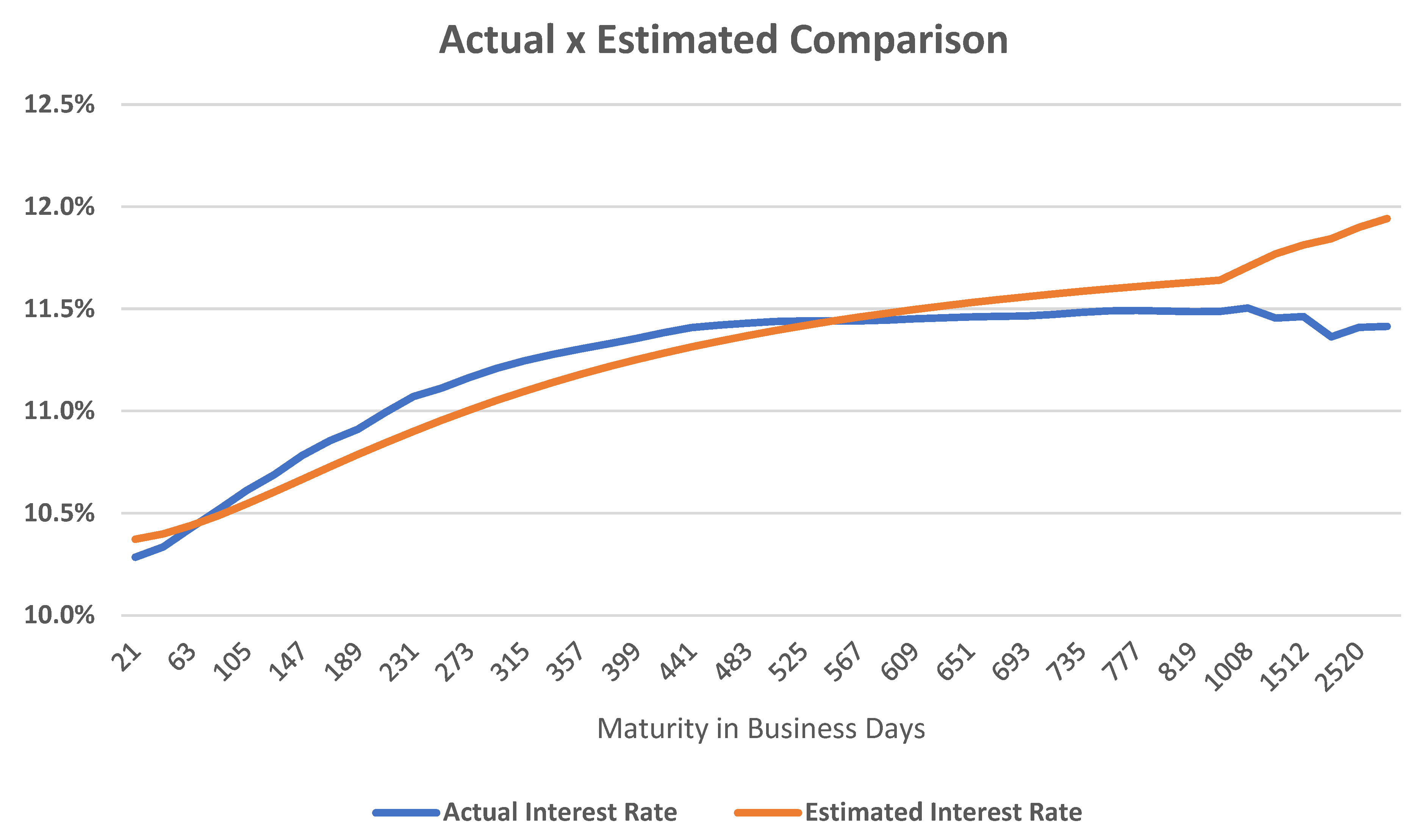
4.2. The Model in Operation

The model was employed to replicate the yield curve over time and assess the discrepancies between the model-generated yield curves and those observed in reality. To quantify these discrepancies, the variance between the model and the observed yield curve was calculated for each maturity, effectively measuring the tracking error of the estimates.
Equation (3), with λ1 = 0.010108 and λ2 = 0.011155, was used to calculate the yield curve for each Friday within the selected period.
As illustrated in the Figure 5, the model’s adherence can be considered reasonable, with an error of ±0.7% per annum for longer terms 68% of the time.
Potential sources of error include the following:
  • Statistical model limitations: Forecasting models inherently have margins of error.
  • Data lag: Information used for forecasting was collected up to Thursday, while interbank deposit futures contracts traded on Friday or subsequent business days. This may result in incomplete information for Friday’s predictions.
  • Time-varying λ terms: The λ terms are influenced by macroeconomic variables, making them dynamic.
  • Residual autocorrelation: The models exhibited residual autocorrelation, suggesting potential deficiencies in statistical specifications and the need for additional explanatory variables.

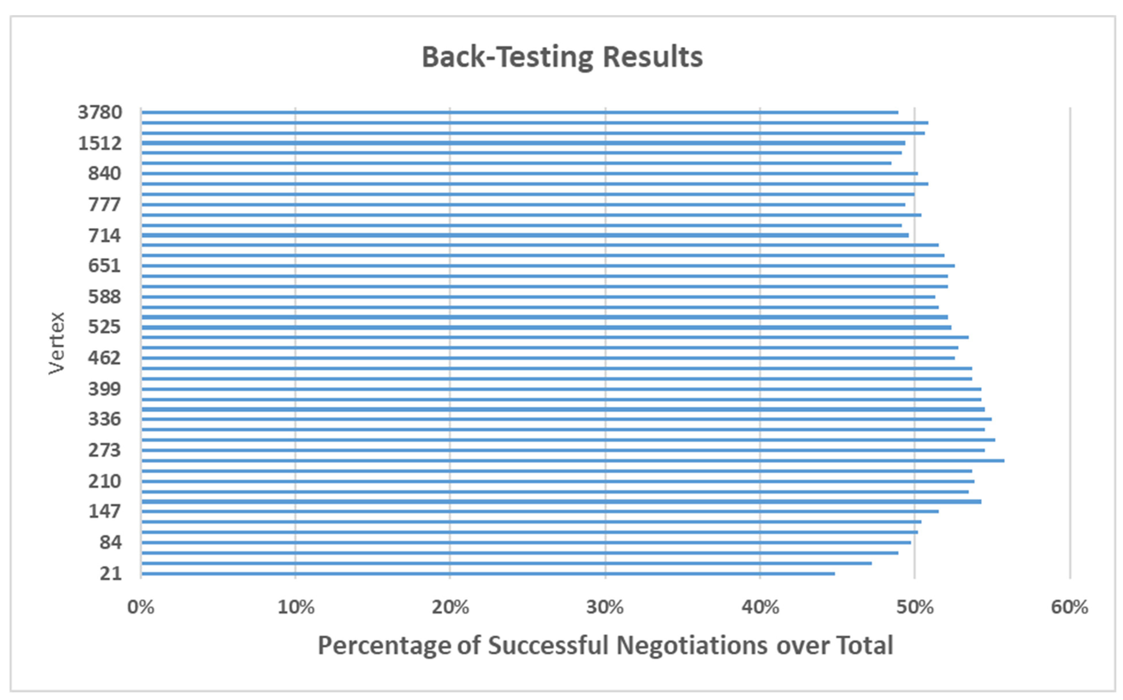
4.3. Usage in Algorithms

To evaluate the model’s ability to consistently estimate yield curve behavior, we compared the Thursday market closing value with the model’s Friday forecast for specific curve vertices. A hypothetical robot trader, triggering purchase and sale orders for interbank-deposit futures contracts, could be used to test the model’s predictions. However, to avoid potential biases from trading and immunization techniques, we conducted an in-sample routine: (a) On Thursday’s market close, the yield curve is known. (b) Additionally, relevant explanatory variables such as the Selic rate, the Focus Bulletin’s expected inflation and GDP rates, exchange rates, and CDS are available. (c) By inputting these variables into the model’s equation, we can forecast the Friday yield curve. (d) Vertices where the forecasted yield curve indicates a higher rate than Thursday’s are marked as “high”. (e) Vertices where the forecasted yield curve indicates a lower rate than Thursday’s are marked as “low”. (f) We then compare the actual Friday rates to the forecasted “high” and “low” designations. A correct prediction is marked as 1, and an incorrect prediction as 0.
The accuracy of the model can be measured by calculating the percentage of correct predictions for each vertex using the sum of the “1’s” obtained. The back-testing results can be visualized in the following graph:
The back-testing methodology employed in Figure 6 followed a systematic approach such as, it used Thursday’s market closing values and explanatory variables to forecast Friday’s yield curve, it marked vertices as “high” or “low” based on predicted movements, it compared predictions to actual Friday rates (1 for correct, 0 for incorrect), and it calculated percentage of correct predictions for each vertex. The model demonstrated levels of success across different maturity points, with the strongest performance in the 1–12 month range, achieving 55–60% prediction accuracy. The most effective predictions occurred in the 168–399 days segment and the performance declined for longer maturities (2–9 years), dropping below 50% accuracy.
The varying performance across vertices reflects some market characteristics showing that very short vertices (under 31.5 business days) show limited surprise due to monetary policy meeting intervals, moreover, longer-term vertices demonstrate reduced accuracy due to lower liquidity, also best results appear in vertices with higher market liquidity, and performance aligns with the most actively traded segments of the Brazilian interest rate futures market.
As the above experiment is equivalent to tossing a coin, its associated probability distribution is a B e p , with p = 50 % .
This distribution can be approximated by a normal distribution, in accordance with the equation
p ^ ~ N p ; p 1 p n
which is good when n p 5 .
Given that n = 4644 and p = 0.5 , a statistical test can be proposed, represented by
H0: 
The model’s prediction accuracy equals random chance (p = 0.5).
H1: 
The model’s prediction accuracy exceeds random chance (p > 0.5).
The results of this test are summarized in Figure 7:
The analysis shown in Figure 7 revealed the strongest predictive performances at 252 days (p-value = 1.22%) and 294 days (p-value = 2.59%). Additionally, it showed a statistically significant predictive power for vertices between 168 and 399 days, and finally, the p-values below 0.10 indicate performance significantly better than random for short/medium-term maturities.
Table 6 contains a summary of the vertices at which the model beats the tossing of a coin for a p-value with a limit of 10%.
The model’s outperformance at vertices between 168 and 399 days is particularly significant because these maturities represent the most actively traded segments of the Brazilian interest rate futures market. The strongest predictive power occurs at 252 and 294 days (with p-values of 1.22% and 2.59%, respectively), which precisely aligns with typical investment horizons in the Brazilian fixed income market. Moreover, these vertices correspond to the most liquid segments of the Brazilian interest rate futures market, where price discovery is most efficient. The model’s effectiveness in these segments is particularly valuable as they represent maturities where most market activity occurs, making the predictions practically applicable for market participants.
The predictive power aligns with Brazil’s monetary policy transmission horizon, making the findings valuable for policy analysis. The results are particularly relevant for analyzing market reactions around COPOM (Monetary Policy Committee) meetings, as these vertices capture both immediate and medium-term policy impacts. These results also corroborate Akram and Uddin (2021).
The findings have practical applications for the development of trading algorithms focused on medium-term rate movements; the use of risk management tools for financial institutions; market analysis around monetary policy events; and support for clearinghouses and financial information providers requiring reliable rate predictions.
Another highlight is that the varying performance across vertices reflects market microstructure aspects, such as very short vertices (under 31.5 business days), and shows less surprise due to monetary policy meeting intervals. On the other hand, longer-term vertices suffer from lower liquidity and rely on interpolation. The most reliable results appear in vertices with higher market liquidity.

4.4. Sensitivity Analysis

It is reasonable to assume that the impact of macroeconomic variables on the yield curve varies across different maturity horizons. The proposed model can be used to qualitatively assess this phenomenon.
To examine how the macroeconomic environment influences the yield curve over time, we focused on the year 2014, the most recent year within our sample. Table 7 presents the regression coefficients for the Svensson model parameters (β0, β1, β2, and β3), specifically for the year 2014, which serves as the baseline for sensitivity analysis. The table demonstrates how different macroeconomic variables influence each parameter of the yield curve.
The Long-term Factor (β0) showed sensitivity to long-term economic indicators and was a primary driver of the overall interest rate level. The Short-term Factor (β1) determined the slope of the yield curve and reflected immediate monetary policy impacts. The First Curvature Factor (β2) explained about 69% of curvature variations (R2 = 0.69), significantly influenced by the Selic rate level (positive relationship), CDS level (positive relationship), and expected inflation changes (negative relationship). And finally, the second curvature Factor (β3) showed similar behavior to β2, also explained approximately 71% of variations (R2 = 0.71), was affected by the same macroeconomic variables as β2, and provided additional flexibility in curve shape modelling.
Table 8 presents the “Variable Vector” containing macroeconomic data for the specific week of 26 September through 2 October 2014, which was used to estimate the Yield Curve for 3 October 2014.
The key components presented at Table 8 are the macroeconomic variables. It can be observed that the Selic rate was 10.90% per annum (10.35% in continuous terms), the exchange rate was an average of BRL 2.455/USD, the weekly variation was BRL 0.0608/USD, the CDS spread was 173.05 basis points, the inflation expectation was 6.31% (Focus Bulletin), the weekly change increased in 0.01 percentage points, and the GDP expectation was 0.92% (Focus Bulletin). The sensitivity testing showed how the yield curve responds to macroeconomic changes; moreover, it demonstrates the model’s predictive capabilities, and it validated theoretical relationships between variables.
When analyzing both tables together (Table 7 and Table 8) it can be observed that the model demonstrated how macroeconomic variables influence yield curve parameters, showed the model’s ability to capture market dynamics, and provided empirical support for theoretical relationships. This model offers a framework for yield curve estimation, shows how to incorporate macroeconomic data into predictions, and provides a tool for market analysis and forecasting. Furthermore, the risk assessment aspect helps understand sensitivity to various economic factors, allows for scenario analysis and stress testing, and supports risk management decisions.
Table 9 presents the calculated beta parameters (β0, β1, β2, and β3) for 3 October 2014, which were derived by multiplying the macroeconomic variables from Table 8 with their corresponding regression coefficients from Table 7. This table demonstrates the practical application of the Svensson model in estimating the yield curve.
The parameters presented in Table 9 show that the Long-term Factor (β0 = 0.1198) represents the asymptotic level of the yield curve and indicates the long-term interest rate level, and the value reflects the combined impact of inflation expectations, GDP growth expectations, and sovereign risk premiums. The Short-term Factor (β1 = −0.0087) determines the slope of the yield curve and the negative value indicates the downward pressure on short-term rates and the potential flattening of the yield curve and is primarily influenced by monetary policy stance. Subsequently, the first curvature factor (β2 = −0.0281) controls medium-term curve dynamics and the negative value suggests a downward pressure on medium-term rates, an adjustment in the curve’s hump shape and reflects market expectations and risk premiums. The second curvature factor (β3 = 0.0187) provides additional flexibility in curve shape, the positive value indicates an upward adjustment in longer-term segments, and the fine tuning of the curve’s shape helps capture complex yield curve patterns.
In relation to the model, it can be observed that these parameters are used to generate the estimated yield curve for 3 October 2014. The resulting curve is compared with actual market observations, and it demonstrates the model’s practical effectiveness in yield curve estimation. Moreover, the model’s performance achieved high goodness of fit, with R2 values above 0.95 and tracking errors remaining within approximately 0.7% annually for longer maturities, and it captures both the shape and level of the yield curve.
Finally, the model suggests that the instantaneous rate (β0 + β1) showed limited dependence on market liquidity conditions. The short-term rates are primarily driven by changes in expected inflation, GDP growth expectations, and monetary policy decisions.
The beta parameters in Table 9 generated the estimated yield curve shown in Figure 8. This comparison with observed rates validates the model’s accuracy and demonstrates the practical utility of the Svensson approach. This comprehensive analysis in Table 9 shows how the model effectively translates macroeconomic conditions into yield curve parameters, providing both theoretical insights and practical applications for market participants.
We generated the estimated Yield Curve below, plotted together with the Yield Curve observed on 3 October 2014:
The comparison between estimated and observed yield curves reveals that the model achieves high goodness of fit, with R2 values averaging above 0.95, tracking errors remaining within approximately 0.7% annually for longer maturities (68% confidence interval), and the model successfully capturing both the general shape and level of the yield curve.
The sensitivity analysis demonstrates how the yield curve responds to various macroeconomic shocks, such as (a) a 100 basis point increase in Selic rate primarily affects the curve’s level; (b) a 10% currency depreciation impacts both slope and curvature; (c) a 3% increase in CDS spreads influences the risk premium component, (d) a 50 basis point increase in inflation expectations affects the forward rate structure; and (e) a 50 basis point increase in expected GDP impacts the medium-term segment.
This analysis reveals that the interest rate level is influenced by Selic rate, exchange rate variations, CDS level, and variations in expected GDP and inflation. Additionally, the slope correlates positively with variations in inflation, GDP, CDS, and expected rates; and the instantaneous interest rate is primarily influenced by expected inflation and GDP variations. Finally, the curvature increases with Selic rate and decreases with positive variations in expected inflation.
The robustness of our findings is supported by a comprehensive body of evidence gathered through rigorous testing and analysis. We utilized a 15-year time series of yield curve data from B3, with the model showing superior performance (measured by R2) compared to the original Nelson–Siegel model. Statistical tests demonstrated better than random predictive ability for certain vertices, particularly in regions of greater statistical significance. Our results aligned with conventional economic theory, despite some residual autocorrelation, and provided empirical validation of how variables like SELIC rate, exchange rate variations, CDS levels, and expected GDP/inflation impact different aspects of the interest rate curve. Moreover, it includes back-testing within the sample, analysis of prediction accuracy compared to random outcomes, and sensitivity analysis for different macroeconomic scenarios. These elements collectively demonstrate that while the data period may not be current, the methodological contributions and structural relationships identified in our study remain valuable for understanding and analyzing Brazilian interest rate term structure.

5. Conclusions

Parsimonious models for fitting yield curves are well-established tools in market finance, employed by clearing houses, financial information providers, central banks, and financial institutions. The approach presented in this study, which involves integrating yield curve fitting with explanatory variables, remains a subject of ongoing academic interest.
Regarding the results obtained, several observations can be made, as while regression analyses generally produce satisfactory explanatory models, autocorrelation of residuals was evident in all cases. However, the stylized facts and signals from the estimators closely aligned with conventional economic theory. Moreover, the regressions relating curve parameters to macroeconomic variables required the inclusion of year-specific dummy variables. This suggests the presence of liquidity conditions and other factors not captured by quantitative or qualitative variables. Future studies could explore the impact of derivative trading volume on the B3 market.
According to the model, the level of interest rates (long-term interest rates) is influenced by the Selic rate, exchange rate variations, CDS level, and variations in expected GDP and inflation rates. An increase in any of these factors leads to an increase in the yield curve level. The slope of the yield curve is positively correlated with variations in inflation, GDP, CDS, and expected GDP and inflation rates. A positive inflation variation tends to yield a positively sloped curve, while a higher Selic rate has a negative impact on the slope. The instantaneous interest rate, a combination of level and slope parameters, is primarily influenced by variations in expected inflation and GDP, but with less intensity than long-term interest rates. Interestingly, it is not affected by liquidity conditions. Long-term rates vary across different years and the joint curvature, determined by the combination of λ1 and λ2, increases with the Selic rate and decreases with positive variations in expected inflation. It is not affected by variations in expected GDP.
This research aimed to model the aggregate behavior of agents involved in interest rate futures contracts and other instruments used to price the Brazilian yield curve, utilizing publicly available macroeconomic variables relevant to the Central Bank of Brazil’s decision-making process regarding interest rates. The Svensson (1994) model, a refinement of Nelson–Siegel’s original technique (Nelson & Siegel, 1987), was employed to fit the yield curve to real data. The regression equations obtained yielded promising results as the relationships between the model’s parameters and macroeconomic variables align with expectations from economic and financial theory. Finally, the model demonstrated predictive power for certain vertices, outperforming purely random events. This predictive power was particularly strong for shorter-term maturities, suggesting that the analysis could be further enhanced by focusing on a shorter time horizon and incorporating additional technical variables.
The primary contribution of our paper is methodological, demonstrating how the Svensson model can be effectively applied to emerging markets like Brazil. The structural relationships we identify between macroeconomic variables and term structure remain relevant regardless of the specific time. The fundamental economic relationships and market dynamics we analyze continue to hold true, as evidenced by the model’s ability to capture how the yield curve responds to changes in key variables such as Selic rate, exchange rate fluctuations, CDS levels, and expected GDP/inflation rates.
Furthermore, the contributions of this research emphasize the market and the economic academy. From a market perspective this study is the first to utilize B3 term structure data from up to 15-year maturities in Brazil, documenting lower precision in longer maturities due to low liquidity. It also demonstrated the Svensson model’s superior ability to capture yield curve sinuosity compared to the Nelson–Siegel model, particularly due to the second parameter. Moreover, the paper suggested that the Brazilian yield curve peaks at approximately one-third the time of the US curve based on decay parameters. The model showed good predictive power, specifically in key trading maturities (between first meeting and one year). From an economic perspective the results in this research documented relationships between macroeconomic variables and yield curve parameters that align with economic theory. Moreover, the research provided empirical evidence on how the Brazilian yield curve responds to changes in policy rate, exchange rate, and inflation expectations.
For future research, the following modifications could potentially improve model performance: selecting the optimal λ1 and λ2 values and considering plotting their joint distribution of R2 values. Furthermore, a restriction of the model to periods with higher liquidity, as liquidity constraints in certain vertices, especially longer ones, can affect the model’s predictive power. Also, we can incorporate additional variables such as the volume of positions in B3 derivatives markets, focusing on one-day interbank deposits. Analyzing the gap between foreign and local investors might also be insightful.

Author Contributions

Conceptualization, J.M.V.N. and C.B.; methodology, J.M.V.N.; software, J.M.V.N.; validation, J.M.V.N., C.B. and R.M.; formal analysis, J.M.V.N. and C.B.; investigation, J.M.V.N. and C.B.; resources, J.M.V.N.; writing—original draft preparation, J.M.V.N. and C.B.; writing—review and editing, J.M.V.N., C.B. and R.M.; visualization, J.M.V.N. and C.B.; supervision, R.M.; project administration, J.M.V.N. and C.B. All authors have read and agreed to the published version of the manuscript.

Funding

This research received no external funding.

Informed Consent Statement

Not applicable.

Data Availability Statement

The original contributions presented in this study are included in the article. Further inquiries can be directed to the corresponding author. Table 1 presents the websites where the public data can be found.

Conflicts of Interest

No potential conflict of interest was reported by the authors.

Notes

1
This public database can be accessed at Brazilian Central Bank’s time series database (www.bcb.gov.br), the Brazilian Treasury’s yield curve data (www.tesourodireto.com.br), and B3’s market data portal (www.b3.com.br). Accessed during 18 November 2015 to 18 December 2015.
2
This public database can be accessed at Central Bank’s Focus Market Report (www.bcb.gov.br/en/focus), B3 BOVESPA’s derivatives trading data, and Bank for International Settlements (www.bis.org) for global market structure analysis. Accessed on 25 February 2025.
3
More information about COPOM (Monetary Policy Committee in Brazil) can be see at https://www.bcb.gov.br/en/monetarypolicy/committee.
4
The methodology employs explanatory variables observed at time t–1 to predict values at time t. This approach helps mitigate potential endogeneity issues in the model. The use of lagged variables necessarily reduces the effective sample size by one observation. Moreover, this methodology requires using Thursday’s market close data to predict Friday’s values. This temporal alignment structure results in the loss of one additional observation. This approach ensures that all relevant information is properly incorporated into the model.

References

  1. Akram, T., & Uddin, S. A. H. (2021). An empirical analysis of long-term Brazilian interest rates. PLoS ONE, 16(9), e0257313. [Google Scholar] [CrossRef] [PubMed]
  2. Amihud, Y., & Mendelson, H. (1991). Liquidity, maturity, and the yields on US Treasury securities. The Journal of Finance, 46(4), 1411–1425. [Google Scholar] [CrossRef]
  3. Ariefianto, D., Amanda, C., & Ananto Husodo, Z. (2024). Term structure of interest rate and macro economy: An empirical study on selected emerging countries sovereign bond. Journal of Capital Markets Studies, 8(2), 195–211. [Google Scholar] [CrossRef]
  4. Bauer, M. D., & Rudebusch, G. D. (2020). Interest rates under falling stars. American Economic Review, 110(5), 1316–1354. [Google Scholar] [CrossRef]
  5. Caldeira, J. F. (2011). Estimação da estrutura a termo da curva de juros no Brasil através de modelos paramétricos e não paramétricos. Análise Econômica, 29(55). [Google Scholar] [CrossRef]
  6. Caldeira, J. F., Cordeiro, W. C., Ruiz, E., & Santos, A. A. (2025). Forecasting the yield curve: The role of additional and time-varying decay parameters, conditional heteroscedasticity, and macro-economic factors. Journal of Time Series Analysis, 46(2), 258–285. [Google Scholar] [CrossRef]
  7. Caldeira, J. F., Moura, G. V., & Santos, A. A. (2015). Measuring risk in fixed income portfolios using yield curve models. Computational Economics, 46(1), 65–82. [Google Scholar] [CrossRef]
  8. Chen, X., Wang, J., Wu, C., & Wu, D. (2024). Extreme illiquidity and cross-sectional corporate bond returns. Journal of Financial Markets, 68, 100895. [Google Scholar] [CrossRef]
  9. Coroneo, L., Giannone, D., & Modugno, M. (2016). Unspanned macroeconomic factors in the yield curve. Journal of Business & Economic Statistics, 34(3), 472–485. [Google Scholar]
  10. Cox, J. C., Ingersoll, J. E., & Ross, S. A. (1985). A theory of the term structure of interest rates. Econometrica, 53(2), 385–407. [Google Scholar] [CrossRef]
  11. Diebold, F. X., & Li, C. (2006). Forecasting the term structure of government bond yields. Journal of Econometrics, 130, 337–364. [Google Scholar] [CrossRef]
  12. Elton, E. J., & Green, T. C. (1998). Tax and liquidity effects in pricing government bonds. The Journal of Finance, 53(5), 1533–1562. [Google Scholar] [CrossRef]
  13. Gomes da Silva, C., Nunes, C. V. A., & Holland, M. (2011). Sinalização de política monetária e movimento na estrutura a termo de taxas de juros no Brasil (pp. 71–90). Escola de Economia de São Paulo, Fundação Getulio Vargas. [Google Scholar]
  14. Hull, J., & White, A. (1990). Valuing derivative securities using the explicit finite difference method. Journal of Financial and Quantitative Analysis, 25(1), 87–100. [Google Scholar] [CrossRef]
  15. Huse, C. (2011). Term structure modelling with observable state variables. Journal of Banking & Finance, 35(12), 3240–3252. [Google Scholar]
  16. Kumar, S., & Virmani, V. (2022). Term structure estimation with liquidity-adjusted Affine Nelson Siegel model: A nonlinear state space approach applied to the Indian bond market. Applied Economics, 54(6), 648–669. [Google Scholar] [CrossRef]
  17. Ludvigson, S. C., & Ng, S. (2009). Macro factors in bond risk premia. The Review of Financial Studies, 22(12), 5027–5067. [Google Scholar] [CrossRef]
  18. McCulloch, J. H. (1971). Measuring the term structure of interest rates. The Journal of Business, 44(1), 19–31. [Google Scholar] [CrossRef]
  19. McCulloch, J. H. (1975). The tax-adjusted yield curve. The Journal of Finance, 30(3), 811–830. [Google Scholar]
  20. Moench, E. (2008). Forecasting the yield curve in a data-rich environment: A no-arbitrage factor-augmented VAR approach. Journal of Econometrics, 146(1), 26–43. [Google Scholar] [CrossRef]
  21. Nelson, C. R., & Siegel, A. F. (1987). Parsimonious modelling of yield curves. Journal of Business, 60, 473–489. [Google Scholar] [CrossRef]
  22. Svensson, L. E. O. (1994). Estimating and interpreting forward interest rates: Sweden 1992–1994 [NBER Working Paper Series 4871]. National Bureau of Economic Research. [Google Scholar]
  23. Tavanielli, R., & Laurini, M. (2023). Yield curve models with regime changes: An analysis for the Brazilian interest rate market. Mathematics, 11(11), 2549. [Google Scholar] [CrossRef]
  24. Tsai, S. C. (2012). Liquidity and yield curve estimation. Emerging Markets Finance and Trade, 48(5), 4–24. [Google Scholar] [CrossRef]
  25. Ullah, W., Matsuda, Y., & Tsukuda, Y. (2015). Generalized Nelson–Siegel term structure model: Do the second slope and curvature factors improve the in-sample fit and out-of-sample forecasts? Journal of Applied Statistics, 42(4), 876–904. [Google Scholar] [CrossRef]
  26. Vasicek, O. (1977). An equilibrium characterization of the term structure. Journal of Financial Economics, 5(2), 177–188. [Google Scholar] [CrossRef]
Figure 1. Histogram λ —Nelson and Siegel Model.
Economies 13 00108 g001
Figure 2. Histogram λ 1 —Svensson Model.
Economies 13 00108 g002
Figure 3. Histogram λ 2 —Svensson Model.
Economies 13 00108 g003
Figure 4. Histogram of the daily R2 values.
Economies 13 00108 g004
Figure 5. Standard-deviation (actual rate–estimated rate) (% p.a.) (axes: error standard deviation (Y) and working days (X)).
Economies 13 00108 g005
Figure 6. In-sample back test of the model’s prediction.
Economies 13 00108 g006
Figure 7. p-values of hypothesis tests on the vertices.
Economies 13 00108 g007
Figure 8. Estimated and observed yield curve on 3 October 2014.
Economies 13 00108 g008
Table 1. Variables information.
DataSourceWebsite (Accessed on 25 February 2025)Period
Interest Rate MarketBrazilian Mercantile & Futures Exchange (B3), now part of B3www.b3.com.br/en_us/market-data-and-indices/Daily data from January 2006 to December 2014
Market Expectations
Expected Inflation (IPCA)Brazilian Central Bank’s Focus Market Reportwww.bcb.gov.br/en/publications/focusmarketreadoutWeekly
GDP growth expectationsBrazilian Central Bank’s Focus Market Reportwww.bcb.gov.br/en/publications/focusmarketreadoutWeekly
Domestic Economic Indicators
Current InflationIPC-FIPE (Consumer Price Index)www.fipe.org.br (São Paulo metropolitan area)weekly
Basic Interest Rate (Selic)Brazilian Central Bank (BCB)www.bcb.gov.brDaily updates
Exchange RateBrazilian Central Bank (BCB)www.bcb.gov.brDaily BRL/USD rate
Risk Measures
Country Risk5-year Brazil Credit Default Swap (CDS) quotesBloombergDaily quotes
Global RiskCBOE Volatility Index (VIX)—Chicago Board Options Exchangewww.cboe.comDaily
International Market
External Interest Rate10-year U.S. Treasury Bills—U.S. Treasury Departmentwww.treasury.govDaily
Commodity IndexCoreCommodity CRB IndexThomson ReutersDaily
Table 2. Total of Best R2 by Model.
Nelson and SiegelSvenssonTotal
224062246
99.70%0.27%100.00%
Table 3. Sample distribution criteria in the model.
VariableFrequency of DisclosureDisclosure DayModel Used
Expected inflationWeeklyFirst working day of the weekWeek t − 1
Expected GDPWeeklyFirst working day of the weekWeek t − 1
SELIC *DailyDailyThursday (Week t − 1)
VIXDailyDailyAverage (Week t − 1)
T-Bill 10 yearsDailyDailyAverage (Week t − 1)
Exchange RateDailyDailyAverage (Week t − 1)
CRBDailyDailyAverage (Week t − 1)
Current inflation (IPC-FIPE)WeeklyFirst working day of the weekconsidered those disclosed until Thursday (week t − 1)
Model betasDaily Friday (week t)
Note: * Brazilian Interest Rate.
Table 4. Summary of regression coefficients.
Variableβ0p-Valueβ1p-Valueβ2p-Valueβ3p-Value
CDS0.0000720.06%−0.0000860.10%−0.0018200.00%0.0017150.00%
DExchangeRate0.0244474.25%−0.0262742.87%----
DIPCA_Focus4.5427320.10%−3.9124880.17%48.6648104.20%−52.5651302.48%
DGDP_Focus1.8481000.48%−1.6566330.75%----
Selic--1.0251720.00%4.6467370.00%−4.4514620.00%
DSelic0.3886810.83%−0.6130910.00%6.4170511.75%−6.0071751.70%
D20060.1242580.00%−0.1246770.00%−0.3421330.00%0.3178610.00%
D20070.1028640.00%−0.1047420.00%−0.3706430.00%0.3517780.00%
D20080.1180930.00%−0.1169240.00%----
D20090.1080870.00%−0.1075910.00%−0.2465280.00%0.1901650.01%
D20100.1075140.00%−0.1072300.00%−0.1090951.26%0.0933012.57%
D20110.1041490.00%−0.1037260.00%−0.2497330.00%0.2338880.00%
D20120.0907970.00%−0.0941860.00%−0.4811330.00%0.4349700.00%
D20130.0956920.00%−0.0978510.00%−0.2939490.00%0.2693580.00%
D20140.1057840.00%−0.1056940.00%−0.1825410.01%0.1640100.01%
Table 5. Regression statistics.
RegressionR2Adjusted R2DW
β00.6940710.6852520.278329
β10.8260360.8206240.293314
β20.7279790.7213730.395231
β30.7109240.7039050.407741
Table 6. Relevant p-values for the model at the vertices.
Vertex
168210252273294315336357378399
p-Value6.33%9.47%1.22%5.12%2.59%5.12%3.27%5.12%6.33%6.33%
Table 7. Model parameters for 2014.
Macro Variableβ0β1β2β3
CDS0.00007−0.00009−0.001820.00172
Selic0.000001.025174.64674−4.45146
Dselic0.38868−0.613096.41705−6.00718
DExchangeRate0.02445−0.026270.000000.00000
DIPCA_Focus4.54273−3.9124948.66481−52.56513
DGDP_Focus1.84810−1.656630.000000.00000
D20140.10578−0.10569−0.182540.16401
Table 8. Variable vector for sensitivity test.
Macro VariableCDSSelicDselicDExchangeRateDIPCA_FocusDGDP_FocusD2014
Value173.0510.35%00.06080.010%0.010%1
Table 9. Betas parameters for 3 October 2014.
Beta Parametersze
β012.03%
β1−1.66%
β2−1.19%
β3−0.50%
Disclaimer/Publisher’s Note: The statements, opinions and data contained in all publications are solely those of the individual author(s) and contributor(s) and not of MDPI and/or the editor(s). MDPI and/or the editor(s) disclaim responsibility for any injury to people or property resulting from any ideas, methods, instructions or products referred to in the content.

