Estimating Interest Rate Setting Behavior in Brazil: A LSTR Model Approach

Abstract

Given limited research on monetary policy rules in emerging markets, this paper challenges the applicability of a nonlinear Taylor rule in characterizing the monetary policy behavior of the Brazilian Central Bank. It also investigates whether and how the process of setting interest rates has been developed in response to contingencies and special events. We extend the linear Taylor rule to a regime-switching framework, where the transition from one regime to another occurs in a smooth way, using a Logistic Smooth Transition Regression (LSTR) approach. In this sense, we empirically analyze the movement of the nominal short term interest rate of the Brazilian Central Bank using quarterly data, covering the period 1994.Q4–2012.Q2. We find that the nonlinear Taylor rule provides a better description of the Brazilian interest rate setting and is consistent with historical macroeconomic events. In particular, our results show that adopting a nonlinear specification, instead of the linear, leads to a costs reduction in terms of fit: 190 basis points in 1995 and 140 basis points in the mid-2002 presidential election campaign in Brazil. Moreover, the Brazilian monetary policy exhibits nonlinear patterns that better captures special events and may contain relevant information rendering it applicable to unusual conditions, i.e., a financial crisis, which require disconnection from the automatic pilot rule and use of judgement to make decision.

1. Introduction

Taylor (1993) [1], in his seminal contribution, proposed a simple monetary policy rule, linking mechanically policy interest rate to deviating of inflation from its target and output from its potential.

The Taylor rule has been a popular gauge for assessing monetary policy performance both advanced economies and emerging economies. At the same time, it is important to bear in mind that the Taylor rule has its limitations and pitfalls. In this respect, variants of Taylor-type regressions have been applied extensively in order to understand and model the behavior of monetary policy for many countries.

Some researchers include a lagged interest rate term to model the monetary policy inertia or interest rate smoothing behavior (Clarida et al. 1998 [2]). Others consider an augmented version of the linear Taylor rule by enclosing other variables in the conduction mechanism of monetary policy. Svensson (2003) [3] proposes an extension of the Taylor rule by incorporating the exchange rate in a rule designed for small open economies. His conclusion is in line with that of Batini et al. (2001) [4], who show that the descriptive power of the Taylor rule augmented by the exchange rate variable is higher than the standard Taylor rule for small open economies (i.e., the UK).

In addition, recent events show that sudden and sharp swings in financial and credit markets can have a potentially large impact on the macroeconomic outlook. However no clear consensus has been reached about whether the Central Banks should or not react to financial imbalances.

The supporters of including a measure of financial frictions into a Taylor-type monetary policy rule (Cecchetti et al. (2000) [5], Blanchard (2000) [6], Borio and Lowe (2002) [7], Goodhart and Hofmann (2002) [8], Chadha et al. (2004) [9], Rotondi and Vaciago (2005) [10], Gilchrist and Zakrajshek (2011) [11] and Stein (2014) [12]) argued that by allowing the articulation of the interest rate to restore and preserve financial aggregate, central banks would better promote financial stability.

On the contrary, Bernanke and Gertler (1999 [13], 2001 [14]), Bullard and Shaling (2002) [15] and Furlanetto (2011) [16] do not agree with adding asset prices to the reaction function.

Paralleling these evolutions of bodybuilding literature, the financial stability measures takes various forms since it can be based on the Credit Spread (Gerlach-Kristen (2004) [17], Piazzesi and Swansson (2008) [18], Faia and Monacelli (2007) [19], Curdia and Woodford (2010) [20]), asset (house) prices, Financial Stock (Christiano et al. (2010 [21], 2014 [22]), Gilchrist and Zakrajsek (2012) [23] and Agénor and Pereira da Silva (2013) [24], etc.). There are also Synthetic financial stability indicators such as financial stress indices (FSIs) and Financial Conditions indices (FCIs) (Goodhart and Hofmann (2001) [25], Montagnoli and Napolitaro (2005) [26] and Carlson, Lewis and Nelson (2012) [27], etc.).

A common feature of the above specifications of the Taylor rule is that they are linear specifications. Although this linear interest rate rule recognizes nowadays a renewed interest, it is not fully adapted to an environment strongly characterized by uncertainty. Indeed, in a context dominated by uncertainty, the evolution of monetary policy over a long period may entail structural changes in the behavior of monetary authorities. The failure to take into account these changes may bias the results. This opens the way to seek alternative policy rules that can provide better results even through macroeconomic structural changes occur continuously and/or the central bank has imperfect knowledge of the dynamic of the economy. Therefore, the recent literature tries to take nonlinearity into account.

A few works on monetary policy are laid to reconsider the monetary policy framework, in view of specific circumstance such as shocks. In addition, most recent studies focused on nonlinear Taylor rules are limited to industrialized countries, especially the US (Conrad and Eife, 2012 [28]; Lee and Son, 2013 [29]; Olsen et al. 2012 [30]), the UK, ECB, Japan and Canada (Kempa and Wilde, 2011 [31]; Kolman, 2013 [32]).

This paper contributes to current monetary debates through justifying why and when the CB adjusts its policy rule, when fitted in the context of financial distress, namely Brazil. In this vein, the aim of this paper is to adopt and extend the methodology proposed by Taylor (1993) [1] to a nonlinear, threshold models allowing to test the ability of financial conditions to best describe the nonlinear dynamics of interest rate in Brazil.

Accordingly, we investigate both linear and nonlinear Taylor-type monetary policy reaction functions in Brazil using inflation, output gap, lagged interest rate and Ted Spread as a proxy of financial stability. We also examine whether monetary policy following nonlinear Taylor rule model could provide additional information over a linear model and to what extent special regimes (currency crisis (Mexican, Asian, Russian), the victory of worker’s party candidate, Lula in mid-2002 and the Subprime crisis) are not detected by a linear Taylor rule.

The road map of the paper is as follows. Section 2 presents a justification of the nonlinear Taylor rule. Section 3 describes the econometric methodology. In Section 4, we present our dataset and we review the empirical result. The final section concludes.

2. The Theoretical Justification of Why a Central Bank Should Follow a Nonlinear Taylor Rule

While linear models dominate empirical econometric research, there are a number of reasons for expecting Nonlinearity in the policy rule, which can be motivated in at least three different ways.

First, the preferences of the policymaker might not be quadratic in output and inflation. There is a growing literature that relax the quadratic preference asymmetric preference specification (Nobay and Peel (2003) [33], Ruge-Murcia (2003) [34], Dolado, Maria-Dolores and Ruge-Murcia (2005) [35], Karagedikli and Lees (2004) [36], Surico (2007) [37], Cukierman and Muscatelli (2008) [38], etc.).

According to this view, the not quadratic (asymmetric) preferences imply that the Central Bank is assigning different weight to upwards and downwards deviations of aggregates from their expected values in its loss function. In contrast, what is important in a quadratic loss function is especially magnitude of deviation and not its sign. Which means that the Central Bankers put equal weights on positive and negative deviations of key macroeconomic variables such as inflation and output from their target values.

The second reason to explain nonlinear Taylor rule is to assume the underlying aggregate supply schedule might be nonlinear. Schaling (1998) [39], Nobay and Peel (2003) [33], and Dolado et al. (2005) [35] among others introduce convexity or concavity in a short-run Philips curve. Such nonlinearity of the Philips curve implies that the cost of decreasing inflation could not be the same in a recession and in an expansion. Eventually, this nonlinearity translates into a nonlinear interest rate adjustment.

Third, monetary policy is made in an environment of substantial uncertainty. Thus, the design of monetary policy rules must take into account of different types of uncertainty. In particular, one form of uncertainty that is ever present is data uncertainty when data are subject to severe measurement errors. As Theil (1958) [40] showed, rules that work well would be to behave “as if” everything was known with certainty. This is known as “certainty-equivalence”.

In addition, when people do not possess complete knowledge about economic circumstances, the Brainard (1967) [41] principle does hold. In his analysis, Brainard (1967) [41] argues that policy should exhibit conservatism in the face of uncertainty.

Facing model and shock uncertainties, economic agents may resort at two approaches to designing monetary policy rules. The first one, they can reduce uncertainty by learning, such a policy concept is known as “an adaptive learning approach” to policymaking, which sheds new light on the classical result of Brainard (1967) [41]. The intuition of this approach is that economic agents improve their knowledge of an economic model through a certain mechanism of learning. The second one, initiated by Hansen and Sargent (2002) [42] corresponds to “robust control approach”. This is a completely different strategy from adaptive learning; the special attention policy makers pay to the worst-case scenario.

In summary, ignoring these types of uncertainties can potentially lead policy astray.

3. Empirical Methodology

A Taylor-type equation has shown to be a popular gauge for assessments of the monetary policy performance of central banks across the world. Its original form could be expressed as follows.

$$i_t=\overline{r}+{\pi }^{\text{*}}+b_{\pi }\left({\pi }_t-{\pi }^{\text{*}}\right)+b_y\left(y_t-y_t^{\text{*}}\right)$$

(1)

i_t represents the nominal short term interest rate. $\overline{r }$ represents the equilibrium real interest rate. ${\pi }^{*}$ represents the target value of inflation. π_t is the inflation rate at time t calculated from the consumer price index (CPI), reflecting cost of acquiring a fixed basket of goods and services by an average consumer. ($y_t-y_t^{*}$) refers to the output gap, defined as the difference between actual output and potential output, which is measured using the Hodrick-Prescott (1997)’s [43] filter. b_π indicates the sensitivity of the interest rate policy to deviations of inflation from its target. b_y represents the coefficient of the reaction of the central bank to the output gap.

The rule recommends that short-term interest rate should rise if inflation π_t rise above its predetermined target or if output y_t increase above its potential level $y_t^{*}$.

In equilibrium, the deviation of inflation and output from their target values is zero and, therefore, the nominal short term interest rate i_t is the sum of the equilibrium real rate $\overline{r }$ plus the target value of inflation ${\pi }^{*}$.

Despite its simplicity, this rule has fitted the data relatively well in the literature. Some studies extend this linear rule by considering the effect of additional variables in the conduct of monetary policy.

Following Clarida et al. (1998) [2] and Rudebusch (2002) [44] among others, we augment the baseline specification by introducing the lagged interest rate that takes into account the inertia of monetary policy.

Clarida et al. (1998) [2] find that the interest rate smoothing parameter enters significantly in the Taylor rule. In fact, the reason of doing so is mainly due to fear to disturbing capital markets which are too sensitive to policy changes and could create financial instability via investors herding behavior, or the need to build consensus to support a policy change.

In addition, recent events show that large swings in financial variables can have a potentially large impact on the macroeconomic outlook. Views differ about whether monetary policy should respond to asset price movements. For instance, Bernanke and Gertler (1999 [13], 2001 [14]) argue that central bankers should pay no attention to asset price misalignments when shaping monetary policy whereas Cecchetti et al. (2000) [5] reach opposite conclusions arguing that volatilities in asset prices can have a significant impact on both inflation and real economic activity, and central banks might improve performance by providing more information. This leads them to argue that asset price misalignments should be used to guide central bank policy.

In this vein, the vice president of the European central bank, Papademos point out that “close monitoring and deeper analysis of asset price movements monetary and credit development…can provide valuable information for the conduct of monetary policy” [45].

For an early work using such financial variable, Castro (2008) [46] extends the Taylor rule to include monetary policy inertia and the financial condition index (computed as a weighted average of the real effective exchange rate (REER), real share price, real property, price as well as credit spread and futures interest rate spread). He shows that the interest setting process involved in response to financial instability.

Since financial variables are an obvious candidate to be admitted into a standard interest rate rule, we employ the TED Spread as a proxy of such concerns. This is calculated as the gap between three-month futures contacts for US Treasuries, as an indicator of risk free investment and three-month contacts for Eurodollars (measured by the LIBOR1), reflecting the credit rating of corporate borrowers.

A Rising TED Spread indicates an increasing default risk and investors will have a preference for safe investments. On contrary, a Falling TED Spread indicates a decreasing default risk and it shows an accelerating look of trust on financial system. Consequently, the TED Spread is a great indicator of perceived economic risk, solvency of financial institutions and perceived health of the banking system.

Thus, the CB usually reacts to such indicator by relaxing monetary policy stance. Therefore, we expect the variable to enter with a negative sign in the Taylor-type rule. This marks a significant point of departure for our paper; using inflation, output gap, lagged interest rate and a proxy for financial explanatory variable in the Taylor rule. To sum up, the main goal of this paper is to track as closely as possible the monetary policy decision making process of Brazilian Central Bank.

The model thus becomes:

$$i_t=a+b_{\pi }{\pi }_t+b_y{y}_t+\rho i_{t-1}+b_e{e}_t$$

(2)

where e_t is the TED Spread as a proxy of financial stability and ρ measures the degree of interest rate smoothing.

Indeed, in a context dominated by uncertainty, the evolution of monetary policy setting over longer period is structurally unstable. The failure to take into account these changes may bias the results. This opens the way to seek alternative policy rules that can provide better results even through macroeconomic structural changes occur continuously and/or the central bank has imperfect knowledge of the dynamic of the economy. Therefore, the recent literature tries to take nonlinearity into account.

To explain this nonlinear behavior, the common solutions used in the literature are the Markov-switching (MS) model and the smooth transition regression (STR) model. Moreover, the STR models have several advantages over the Markov-switching regime models by allowing gradual evolution of the model’s coefficients and do not impose restrictions on the way parameters vary over time. If a linear functional form were correct, the STR would exclude nonlinear effects and the linear specification outperforms the nonlinear one. Instead, if some nonlinearity exists, the STR technique allows one to choose both the appropriate switching variable and type of the transition function without entailing restrictions on the speed, the intensity and the persistence of the changes. Consequently, we follow the STR approach in the current paper.

Following the work of Teräsvirta (1998) [47], the standard two-regime LSTR for a nonlinear Taylor rule could be derived as follows:

$$i_t= \phi Z_t+ \theta Z_{t}G\left(\gamma ,c,S_t\right)+ u_t, t=1,\dots ,T$$

(3)

where $G\left(\gamma ,c,S_t\right)={(1+\text{exp}\left\{-\frac{\gamma }{{\sigma }_{S_t}^k}{\displaystyle \prod }_{k=1}^k(S_t-c)\right\})}^{-1}$ with γ > 0.

$Z_t=\left(w_t^{\text{'}},x_t^{\text{'}}\right)$ is a vector of regressors including the exogenous variables, $x_t=\left(1,x_{1t},\dots ,x_{kt}\right)$ and lagged dependent variable, $w_t=\left(y_{t-1},\dots ,y_{t-p}\right)$.

The vectors $\phi =\left({\phi }_0,{\phi }_1,\dots ,{\phi }_n\right)$, $\theta =\left({\theta }_0,{\theta }_1,\dots ,{\theta }_m\right)$ represent $\left(\left(n+1\right)*1\right)$ and $\left(\left(m+1\right)*1\right)$ parameter vectors in the linear and nonlinear parts of the model, respectively. The disturbance term is iid with zero mean and constant variance, $u_t\to iidN\left(\theta ,{\sigma }^2\right)$. $G\left(\gamma ,c,S_t\right)$ is the transition function bounded by 0 and 1, and depends upon the transition variable S_t, the slope parameter γ and the location parameter c.

In terms of the above equation, the transition variable increases in tandem with the logistic function. Van Dijk et al. (2002) [48] demonstrate that as $S_t\to 0\left(or \infty \right)$, the transition function becomes abrupt, such that the model becomes indistinguishable from the linear autoregressive model.

Teräsvirta (1994) [49] proposes some procedures to build an STR model; these include linearity test, estimation and evaluation of the model. A linearity test is performed for the purpose of choosing the appropriate transition variable S_t and the most suitable form of the transition function among LSTR1 (with a single transition variable), LSTR2 (with two transition variables) and ESTR. In fact, the null hypothesis of linearity can be formulated as follows:

The null hypothesis of linearity consists in testing $H_0:\theta =0$ in Equation (3) against the alternative hypothesis of nonlinearity: $H_1:\theta \ne 0$.

Luukkonen et al. (1988) [50] argue that testing for linearity is not a straightforward task, due to the fact that the model is only identified under the alternative of nonlinearity. In particular, the parameters c and θ are nuisance parameters and are not present under the null of linearity. Teräsvirta (1998) [47] shows that this identification problem can be circumvented by approximating the transition function with a third Taylor expansion around $\gamma =0$. After reparametrization and rearrangement the approximation yields the following regression:

$${\text{i}}_{\text{t}}={\text{δ}}_0+{{\text{δ}}^{\prime }\tilde{\text{Z}}}_{\text{t}}+{\text{β}}_1^{\text{'}}{\tilde{\text{Z}}}_{\text{t}}{\text{S}}_{\text{t}}+{\text{β}}_2^{\text{'}}{\tilde{\text{Z}}}_{\text{t}}{\text{S}}_{\text{t}}^2+{\text{β}}_3^{\text{'}}{\tilde{\text{Z}}}_{\text{t}}{\text{S}}_{\text{t}}^3+{\text{v}}_{\text{t}}$$

(4)

Accordingly, the null hypothesis of linearity becomes: ${\beta }_1^{\text{'}}= {\beta }_2^{\text{'}}= {\beta }_3^{\text{'}}= 0$ and a LM-type test with F-distribution is used to test this null hypothesis of linearity. Teräsvirta (1998) [47] suggests a linearity test for each candidate transition variable. In terms of this approach, the variable with the lowest p-value (strongest rejection of linearity) is chosen as the transition variable.

Once the linearity is rejected against LSTR-type nonlinearity we follow Teräsvirta (2004) [51] and consider the following three tests:

$$H_{02}:{\beta }_3=0,H_{03}:{\beta }_2=\frac{0}{{\beta }_3}and{H}_{04}:{\beta }_1=\frac{0}{{\beta }_2}={\beta }_3=0$$

The above test statistics are labeled F₂, F₃ and F₄ respectively and are used to determine the number of regime shifts among LSTR1 and LSTR2. The decision rule is that the LSTR1 is chosen if the p-value of H₀₄ or H₀₂ is the lowest. Conversely, the LSTR2 is selected if the p-value of H₀₃ is the lowest.

The chosen model can then be estimated and evaluated as outlined in Eitreheim and Teräsvirta (1996) [52]. Several misspecification tests are used in the STR literature, such as test of no remaining nonlinearity, no residual autocorrelation and parameter constancy. These tests will be carried out in the empirical section.

4. Estimation Results

4.1. Data Description

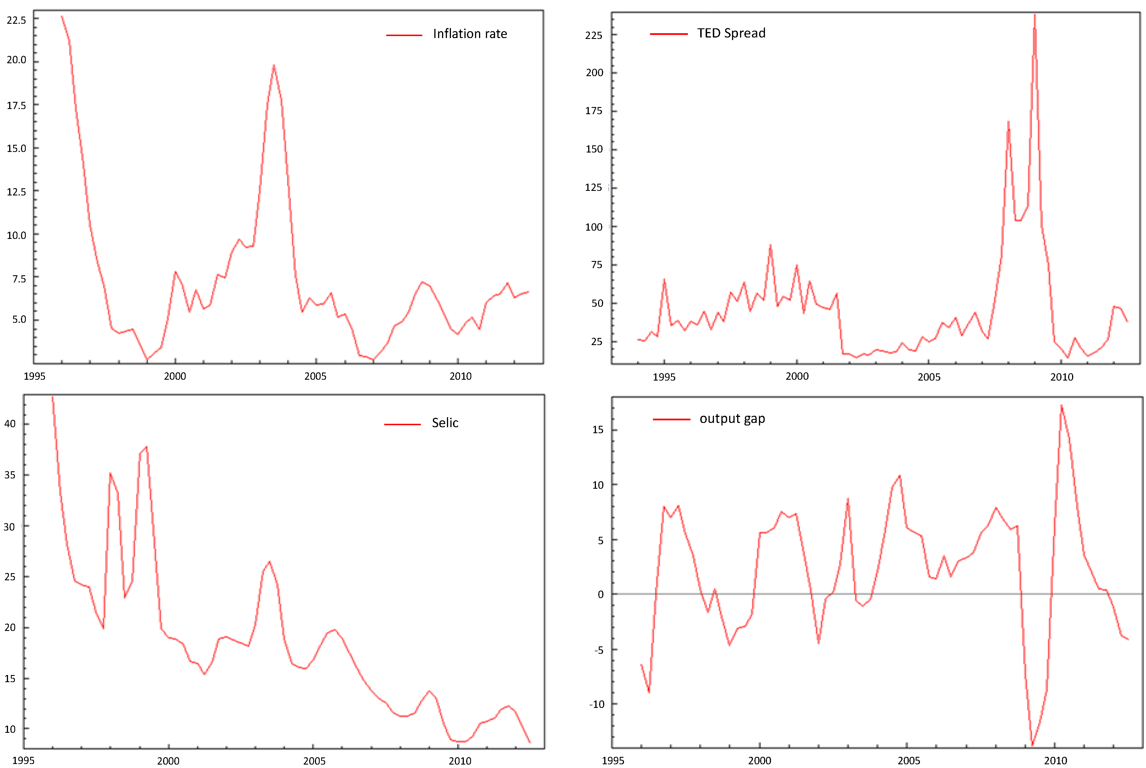
We use quarterly data over the period from 1994.Q4 to 2012.Q2. The data series, which includes the interest rate, inflation rate, output gap and the Ted Spread, is collected from International Financial Statistics (IFS) and Bloomberg databases. The period under investigation begins with the launch of the plano Real in 1994. It is interesting to note that during this period, there was a focus on a set of economic indicators, such as REER, credit spread, asset prices, output gap, balance of payments and fiscal policy.

Figure 1 shows that the plano Real was very successful in exterminating hyperinflation, which had stood at digit levels on an annualized basis and reached simple figures by 1995.

In July 1999, the country moved to an inflation targeting regime. The first time that the target was reached was in the period from 2004 to 2006 after the failure in 2001–2003. Most of this success can be credited to the massive appreciation of Brazilian Real during this period.

The movements in inflation are closely mirrored by the interest rate, the dynamics of which closely follow those of the inflation rate. During the currency crisis periods (Mexican, Asian and Russian), the domestic interest rate (Selic) increased remarkably to avoid further losses in foreign reserve.

With regard to the dynamic of the output gap, different episodes exist. In fact, the output gap experienced a period of high swings and moved from almost (−12) to (12) between 1994 and 2006. During the financial crisis, the output gap experienced a decrease but then increased rapidly, reaching a peak of 16 in 2011.

The general path of TED Spread showed a significant upward trend over the period 2007–2010, with the onset of the Sub-prime crisis in August 2007.

We note that a preliminary analysis suggests that all the considered time series follow a stationary process. Only the ADF test does not reject the null for the Ted Spread, with values of test statistics of around −1.5774. However, in line with common practice, the Ted Spread is treated as stationary.

Overall, the results indicate that at 1% and 5%, the regression conducted by these variables is not spurious. There is no need to difference them when estimating.

Figure 1. Time series dynamics.

Figure 1. Time series dynamics.

4.2. Linear Specification Results

The estimation results of the linear Taylor rule augmented simultaneously by the lagged monetary policy, and the TED Spread, are presented in Table 2.

Table 2. Estimation results of linear augmented Taylor rule.

	Estimate	Standard error
a	−5.531	146.642
bπ	0.137 **	0.352
bv	0.628 ***	15.822
be	−1.566 *	0.144
ρ	−0.737 ***	0.125
AIC	4.432
R2	0.545
ARCH (8)	1.8218	0.784

Note: This table reports the estimates of the linear Taylor rule augmented jointly by the lagged policy rate and the TED Spread considered in this paper. ***, ** and * indicate significance at the respective significance levels 1%, 5% and 10%.

Table 2. Estimation results of linear augmented Taylor rule.

	Estimate	Standard error
a	−5.531	146.642
bπ	0.137 **	0.352
bv	0.628 ***	15.822
be	−1.566 *	0.144
ρ	−0.737 ***	0.125
AIC	4.432
R2	0.545
ARCH (8)	1.8218	0.784

Note: This table reports the estimates of the linear Taylor rule augmented jointly by the lagged policy rate and the TED Spread considered in this paper. ***, ** and * indicate significance at the respective significance levels 1%, 5% and 10%.

Results in Table 2 show that all estimates are significant and have the expected signs. However, these coefficients are less than one, which violates the stability condition in the Taylor rule. Additionally, according to the R2 criteria, we notice a bad overall fit of the model. In addition, the residuals of the estimated linear augmented Taylor rule are Gaussian and not heteroscedastic, which indicates the absence of an ARCH effect in the residuals.

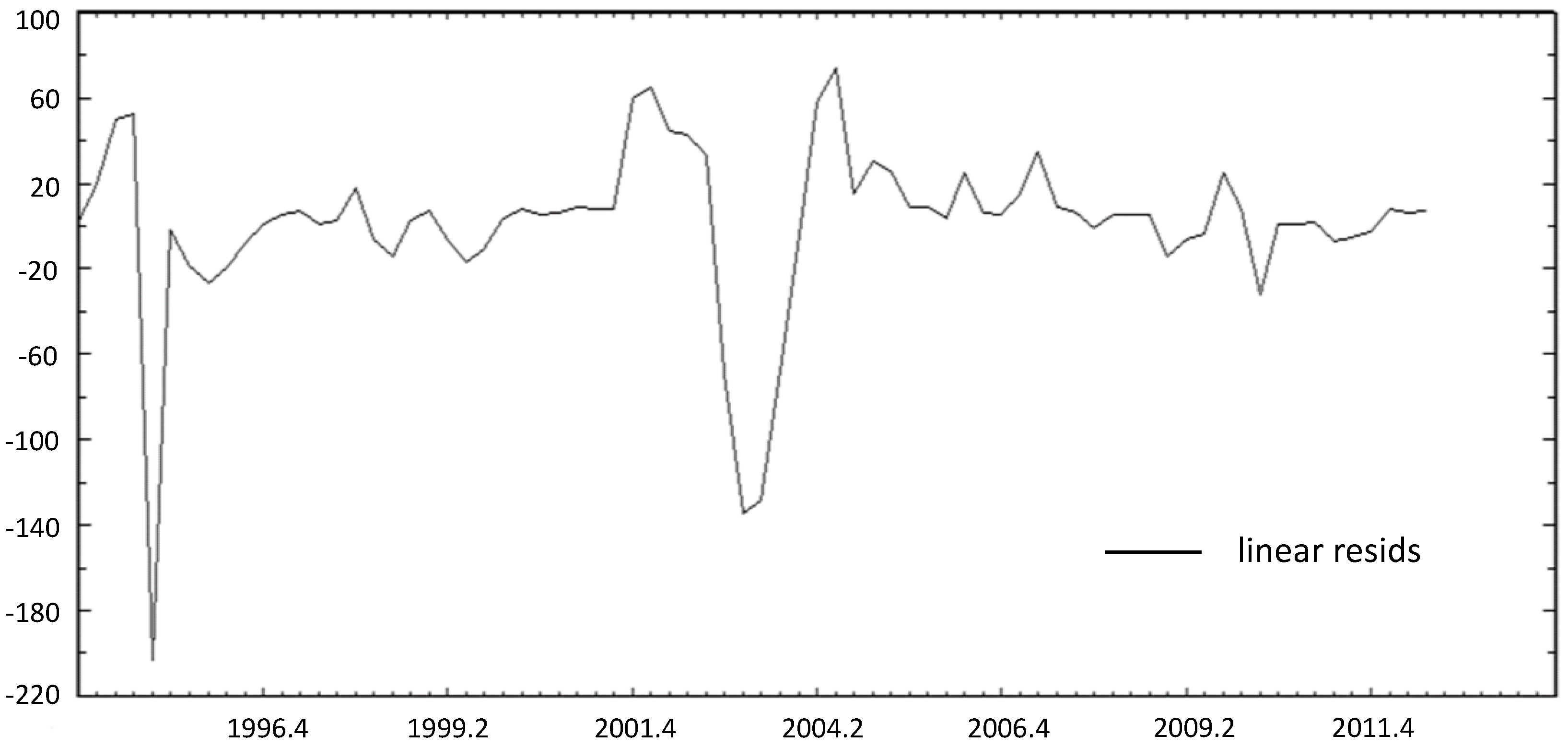
Moving to the graphical analysis (Figure 2), we plot the residuals series form of the regression of Equation (1).

At first sight, Equation (1) seems to fit the Brazilian actual policy rule remarkably well. However, it is interesting to note that there are large residual spikes for more than one period notably in 1995–1996, 2002–2003, 2008–2009 and 2010–2011. The fitted interest rate is, over these time intervals, correlated and remarkably different from the actual value.

Figure 2. Residual plot from Equation (2).

Figure 2. Residual plot from Equation (2).

Negative (positive) residuals correspond to periods when the estimated rule leads to a higher (lower) interest rate (Selic) than the actual ones. Accordingly, in such periods monetary policy appears to have been tightened (relaxed) beyond what was suggested by the inflation, the output gap, the lagged interest rate and the TED Spread deviations. This could be explained by the fact that a linear Taylor rule even augmented is not able to perfectly describe the conduct of monetary policy in the presence of unusual contingencies (Alcidi et al. (2011) [53] and Baaziz et al. (2013) [54]).

Interestingly, this time spam coincides with periods where monetary policy makers had to face the presence of unexpected contingencies. For example, the period 1995–1998 is associated with the currency crises (Mexican, Asian, Russian), that had severe negative spillover effects on Brazil.

Similarly, the Brazilian economy had been heavily influenced by the looming victory of the worker’s party candidate, Lula, which led to new economic tensions as international investors realized that suddenly Lula would default on Brazil’s macroeconomic policies.

Further, the Subprime crisis and its aftermath highlighted the consequence of Brazilian outdated financial institutional design.

At last, with the building zero lower bound in advanced economies since the subprime financial crisis and because of its high interest rate, its open capital account and its floating exchange rate regime, Brazil attracts more and more speculative capital flows.

The main danger induced by these capital inflows is rather linked to massive appreciation of Brazilian currency, what penalizes the Brazilian exportation of manufactured products and increasing the deindustrialization process.

Faced with such risk, the Banko Central do Brazil set up a series of measures to discourage inflows; starting by requiring banks to make a deposit reserve equal to 60% on their dollar selling position. Additional restrictions were put in place is to increase the Financial Operation tax, known as the (IOF).

In summary, we can deduce that although the linear Taylor rule describes well the board contours of Brazil’s behavior, it fails to detect significant changes in policy direction in response to the unusual contingencies which affected the economy of Brazil. Thus, the actual presence of finer monetary regimes corrupts the descriptive power of linear rules even augmented by the lagged policy rate and TED Spread.

The theoretical basis of the linear rule comes from the assumption that policymakers have a quadratic and symmetric loss function and that the aggregate supply or Phillips curve is linear. However, in reality, this assumption is unrealistic; monetary authorities may have asymmetric preferences (Surico, 2007, [37]) and the underlying aggregate supply schedule might be nonlinear leading to a nonlinear adjustment of the policy rate (Dolado et al. 2005 [35]).

Therefore, a nonlinear Taylor rule may be more appropriate to explain the behavior of monetary policy, and therefore the adoption of a nonlinear specification instead of the linear one would leads to fewer errors.

To get a deeper understanding of this phenomenon and investigate to what extent concerns of monetary policy makers are related to unexpected events, we adopt the LSTR model to test the hypothesis that the strength of the response of monetary policy to macroeconomic conditions depends on the level of risk facing the economy.

4.3. Nonlinear Specification Results

The results of the tests for the selection of the transition variable candidates are reported in Table 3.

Table 3. Testing Linearity against STR results.

	F	F4	F3	F2	Selected Model
yt	4.0336 × 10−1	8.7952 × 10−1	2.0809 × 10−1	2.0352 × 10−1	Linear
et *	9.6382 × 10−7	6.2954 × 10−6	4.2514 × 10−1	2.3134 × 10−3	LSTR1
πt	2.1695 × 10−2	7.0021 × 10−2	7.5068 × 10−2	1.6595 × 10−1	LSTR1
it−1	2.5804 × 10−1	4.6102 × 10−2	7.7489 × 10−1	6.4417 × 10−1	Linear

Note: This table reports the results of the test of linearity against the STR nonlinearity. All numbers in this table are p-values associated with the test. F refers to the test of linearity against LSTR while, F2, F3 and F4 allow to select the adequate LSTR model among LSTR with one threshold (LSTR1) and LSTR with two thresholds (LSTR2).

Table 3. Testing Linearity against STR results.

	F	F4	F3	F2	Selected Model
yt	4.0336 × 10−1	8.7952 × 10−1	2.0809 × 10−1	2.0352 × 10−1	Linear
et *	9.6382 × 10−7	6.2954 × 10−6	4.2514 × 10−1	2.3134 × 10−3	LSTR1
πt	2.1695 × 10−2	7.0021 × 10−2	7.5068 × 10−2	1.6595 × 10−1	LSTR1
it−1	2.5804 × 10−1	4.6102 × 10−2	7.7489 × 10−1	6.4417 × 10−1	Linear

Note: This table reports the results of the test of linearity against the STR nonlinearity. All numbers in this table are p-values associated with the test. F refers to the test of linearity against LSTR while, F2, F3 and F4 allow to select the adequate LSTR model among LSTR with one threshold (LSTR1) and LSTR with two thresholds (LSTR2).

Considering the above results, we conclude that there is strong evidence against the linear specification of the Taylor rule and that the behavior of the lagged interest rate, the output gap and the TED Spread, which are likely to be responsible for nonlinear behavior of BCB. Thus, the nonlinear specification can be defined using these variables as possible transition variables in the reaction function, implying that the response of interest rates to inflation, the output gap, the lagged interest rate and TED Spread depends on the inertia of monetary policy regime, the business cycle (recession/expansion) or financial conditions (crisis period/tranquil period).

With regard to the choice of the adequate transition variable, the selected variable is the TED Spread because it provides the lowest p-value of the computed F-statistics for the rejection of the null hypothesis of linearity. Therefore, switching between regimes is controlled by the financial conditions.

This is consistent with Alcidi et al. (2011) [53] identification of transition variable. They identify and use the BAA credit spread as a threshold variable. Thus the switching between regimes is controlled by concerns of the Fed about the health of the financial system.

According to the results in Table 3, the resulting nonlinear LSTR model to be estimated is reported in Equation (5) below:

$$i_t=a_1+{\rho }_1{i}_{t-1}+b_{\pi .1}{\pi }_t+b_{y.1}{y}_t+b_{q.1}{e}_t+(a_2+{\rho }_2{i}_{t-1}+b_{\pi .2}{\pi }_t+b_{y.2}{y}_t+b_{q.2}{e}_t)G(\gamma ,c,e_t)$$

(5)

LSTR model estimation results are reported in Table 4.

Table 4 confirms our conjectures; the estimates clearly reveal the existence of two regimes. The first regime is very close to the linear augmented rule reported in Table 2 while the second (that we will call the low interest rate regime) is at odds with the classical Taylor rule.

Table 4. Estimation results of LSTR model.

	Linear Part	Nonlinear Part
Intercept	57.878 *** (2.5412)	−129.8199 *** (−5.2826)
Selic (t − 1)	5.9412 *** (−4.0315)	2.41042 *** (7.064)
ygapt	3.03015 *** (−1.7236)	1.50074 *** (2.6430)
Inflation rate	0.24434 (0.8373)	0.3857 * (−1.3216)
TED Spread	−0.06 * (−0.0569)	0.0814 *** (5.327)
Gamma	10.006 *** (7.7418)
c	29.73066 *** (36.4122)
AIC	−1.534
R2	99.98%
Jarque-Bera	318.0837 [0.000]
ARCH(8)	15.3961 [0.519]

Note: This table reports the estimates of the nonlinear Taylor rule. Standard errors are between () and p-values are between [ ]. ***, ** and * indicate significance at the respective significance levels 1%, 5% and 10%.

Table 4. Estimation results of LSTR model.

	Linear Part	Nonlinear Part
Intercept	57.878 *** (2.5412)	−129.8199 *** (−5.2826)
Selic (t − 1)	5.9412 *** (−4.0315)	2.41042 *** (7.064)
ygapt	3.03015 *** (−1.7236)	1.50074 *** (2.6430)
Inflation rate	0.24434 (0.8373)	0.3857 * (−1.3216)
TED Spread	−0.06 * (−0.0569)	0.0814 *** (5.327)
Gamma	10.006 *** (7.7418)
c	29.73066 *** (36.4122)
AIC	−1.534
R2	99.98%
Jarque-Bera	318.0837 [0.000]
ARCH(8)	15.3961 [0.519]

Note: This table reports the estimates of the nonlinear Taylor rule. Standard errors are between () and p-values are between [ ]. ***, ** and * indicate significance at the respective significance levels 1%, 5% and 10%.

The TED Spread is chosen to be the threshold variable because of the important weight that the central bank places on this variable and because this variable provides the lowest p-value for the rejection of the linear model. This means that the reaction of BCB to shocks depending on whether the level of the TED Spread is above or below the threshold value of 29.73.

The transition speed parameter is statistically significant and has an estimated value equal to 10.006 indicating a smooth change from one regime to another. Indeed, from the estimated LSTR model.

Our estimates suggest that the parameters of the monetary policy rule seem to change overtime. We report that $1>b_{\pi .2}>b_{\pi .1}$. This result indicates a strong reaction of the Banko central do Brazil to inflation in the high-TED Spread regime while it did not do so in a tranquil period. We also note that the Taylor principle is not satisfied in either regime; the estimated coefficient on inflation is always lower than one, which indicates accommodative behavior of the interest rate to inflation.

We also note that $b_{y.2}<b_{y.1 }$, indicating an asymmetric response from the BCB to the output gap. A plausible explanation is that for a period of financial distress, the monetary authority is concerned about the expense of inflationary pressures, even at the expense of recession.

The results also reveal that ${\rho }_2<{\rho }_1$; that is, there an accommodative response to the inertia of monetary policy during the crisis period rather than in more routine circumstances.

Additionally, $b_{e.2}>b_{e.1}$, suggesting that, as the Ted Spread is on the rise, the Banko central do Brazil pays close attention to the TED Spread when establishing the interest rate. The response to this variable depends on the financial stability. This is in line with the finding of Alcidi et al. (2011) [53] for the case of the Fed which he argues that the Spread between Moody’s BAA corporate bond index yield and 10-year US Treasury note yield play a role in the monetary policy reaction function of the Fed.

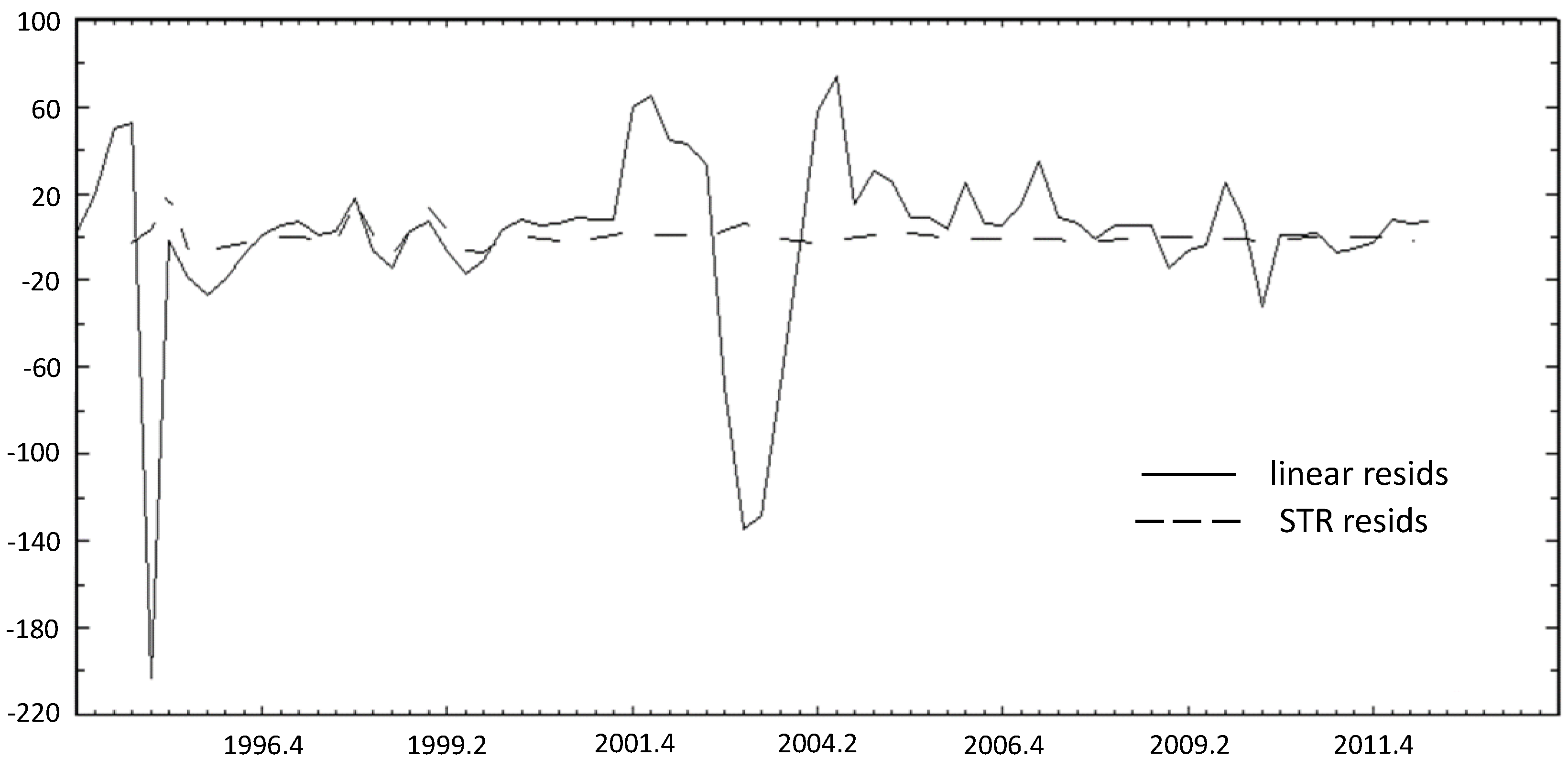
In order to better appreciate the gain in terms of fit obtained by leaving the linear rule for the nonlinear specification, we plot in Figure 3 both the residuals from the augmented linear Taylor rule and the nonlinear specification; we notice that allowing for the functional form to deviate from a constant parameter Taylor rule allows to catch well the broad contours of monetary policy conduct especially in periods of special regime and reveals less autocorrelation of the residuals compared with the linear Taylor rule.

Figure 3. Residual plot from the linear and LSTR models.

Figure 3. Residual plot from the linear and LSTR models.

These results indicate that even if a linear Taylor rule describes the broad contours of monetary policy conduct of BCB, the rule fails to detect significant changes in policy direction following the effects of currency crisis periods (Mexican, Asian and Russian) and the effect of global financial crisis.

These findings suggest that adopting a nonlinear specification instead of a linear one leads to a reduction in errors of 190 basis points in 1995 and 140 basis points in the mi-2002 presidential election campaign in Brazil.

We perform misspecification tests to check for the robustness of our results and determine whether there is an evidence of parameter instability, non-normality of residuals, and remaining nonlinearity. These tests have been proposed by Eitrheim and Teräsvirta (1996) [52]. The results of these tests are presented in Table 5.

Table 5. Diagnostic tests.

Parameter Constancy Test
Transition Variable	F-statistic		p-value
H1	6.4372		0.0015
H2	5.1652		0.0078
H3	4.731		0.0132
No Remaining Nonlinearity
Transition Variable	F	F2	F3	F4
et	5.85 × 10−3	1.031 × 10−1	6.135 × 10−3	3.731 × 10−1

Note: This table reports the diagnostic tests of parameter constancy and no remaining linearity. With regard to the parameter constancy test, H1, H2 and H3 refer to the three functional forms of the transition function considered by Eitrhem and Teräsvirta (1996) [51]. The no remaining linearity test uses the sequence of the F-statistics.

Table 5. Diagnostic tests.

Parameter Constancy Test
Transition Variable	F-statistic		p-value
H1	6.4372		0.0015
H2	5.1652		0.0078
H3	4.731		0.0132
No Remaining Nonlinearity
Transition Variable	F	F2	F3	F4
et	5.85 × 10−3	1.031 × 10−1	6.135 × 10−3	3.731 × 10−1

Note: This table reports the diagnostic tests of parameter constancy and no remaining linearity. With regard to the parameter constancy test, H1, H2 and H3 refer to the three functional forms of the transition function considered by Eitrhem and Teräsvirta (1996) [51]. The no remaining linearity test uses the sequence of the F-statistics.

On the basis of these diagnostic tests, we fail to reject the hypothesis of normality. In addition, the null hypothesis of “there is a conditional heteroskedasticity” is rejected. Thus, we assume that there is no ARCH effect in the residuals.

Moreover, the remaining nonlinearity test shows that some of the nonlinearity was absorbed by an LSTR model with two regimes. Therefore, we come to find evidence for the validity of our empirical nonlinear model. In addition, the parameter constancy test shows that the parameters do not vary over time. These various results therefore confirm the idea that the monetary policy followed by the BCB exhibits some nonlinearity.

5. Conclusions

This paper has shed more light on challenging the suitability of the nonlinear Taylor rule in characterizing the behavior of the Brazilian Central Bank, especially in periods of financial distress.

Using monthly data from 1994 to 2012 to analyze the movement of the nominal short term interest rate for Brazilian Central Bank, we confirm the occurrence of nonlinearity in the Taylor rule. The contribution of this paper is two-fold. First, it support the idea that the nonlinear Taylor rule improves its performance with the advent of currency crisis (Mexican, Asian and Russian) and the effect of presidential election campaign that unfolded in Brazil since mid-2002, providing the best description of the BCB’s interest rate setting behavior.

Second, it provides evidence that the Brazilian policy-makers pay close attention to the financial stability when establishing interest rate.

We conclude that for the analysis of historical monetary policy, the LSTR approach is a viable alternative to track actual interest rate movements to linear reaction function. Building on this view, this paper has provided evidence that it is possible to characterize the behavior of the Brazilian Central Bank as two-state Taylor rule with different coefficients depending on whether the Ted Spread is below or above the estimated threshold value of 29.73. This means that when this financial indicator index exceeds that value, monetary policy enters the finer regime (period of financial distress). These finer regimes require disconnection from the automatic pilot rule of the Central Bank and involving a range of judgmental factors that cannot be condensed into a parametric approach when setting monetary policy decision.

Overall, we can infer from this study that the nonlinear models outperform the linear ones in the sense that the linear specification, by imposing a unique constant regime over the entire sample, fails to capture the special events and unexpected contingencies. In particular, adopting a nonlinear specification instead of the linear leads to a costs reduction in terms of fit: 190 basis points in 1995 and 140 basis points in the mi-2002 presidential election campaign in Brazil.