Abstract
The objective of this paper is the joint application of two different methodological concepts for the detection of lead-lag relationships in economic time-series in order to investigate their consistency and their potential complementarity. The first methodology, a time domain analysis based on vector error correction model, provides evidence about the existence of long-run equilibrium of the time-series and the short-run lead-lag behaviors. The second methodology, a time-frequency concept based on the phase difference of the cross-wavelet coherence, analyzes the lead-lag relationships across various timescales and reveals the altering of leadership over time. The two methods are applied to time-series of wealth-to-income ratio of four developed countries over the period 1970–2010 and analyze the lead-lag relationships of the countries in the long-run and in the short-run. The results show that the two methods are consistent in their major long-run findings, however, they reveal different aspects regarding the short-run dynamics of the lead-lag relationships. Furthermore, the results suggest the complementarity of the two methodologies in the context of a complete framework for the analysis of the lead-lag relationships in non-stationary economic time-series.
Keywords:
lead-lag relationships; vector error correction model; wavelet coherence; wealth-to-income ratio JEL Classification:
N30; O57
1. Introduction
Lead-lag relationships, also known as leader-follower relationships, between economic time-series have been extensively researched in studies of empirical economics and finance. A characteristic example of such relationships constitutes the link between the stock market and oil prices which has been examined both within-in a country (Cong et al. 2008) and across countries (Rault and Arouri 2009). Another example is the link between the index futures and the cash market, where many researchers have found that the futures market leads the cash market (Gwilym and Buckle 2001; Stoll and Whaley 1990). A number of empirical studies have established leader-follower relationships across portfolios, particularly when formed on a size-related basis (Campbell et al. 1997). From another perspective, the leader-follower outcomes regarding economic and market interdependences can be considered as indicators of the economic cycles holding important implications for their determination and tracking of recession periods and of business cycles (Estrella and Mishkin 1998) and are of considerable interest to academics, regulators and practitioners. The dynamics of lead-lag relationships, including the altering of leadership over time, has been also examined in the bibliography (Ajayi and Mougouė 1996; Koutmos 1996). The literature review paper of (Zavadska et al. 2018) focuses on the lead-lag relationship between spot and future prices of crude oil and its historical behavior. The authors highlight a key controversy within the extant literature, as to whether spot or futures prices are the main crude oil price indicator. The literature review indicates that the lead-lag relationship between the variables is a dynamic one, especially during periods of sustained uncertainty, which leads to significant disagreements among researchers regarding the price that plays a dominant role. The lead-lag relationship between crude oil spot and futures markets is a debatable issue, as can be confirmed in the many publications on this topic since the paper by (Silvapulle and Moosa 1999). Changes in spot and futures prices may be due to fundamental shifts in supply and demand; but they could also be due to speculation (Polanco-Martínez and Abadie 2016). Other examples of studies providing evidence for dynamic lead-lag relationships between economic variables include the link between the euro area sovereign bond yield spreads against Germany and their underlying determinants (Afonso et al. 2015) and the study of the determinants of sovereign bond yield spreads across 10 countries of the European economic and monetary union (Bernoth and Erdogan 2012).
In terms of methodology, there are two main methodological pillars for the detection of lead-lag relationships: the time domain methodologies and the time-frequency domain methodologies. The research devoted to the detection and the modeling of lead-lag relationships between economic variables using the traditional methods in the time domain is voluminous. However, the traditional methodologies fail to capture the time-varying (dynamic) nature of the lead-lag relationships. Such approaches require the condition of stationarity of the studied series. In addition, the typical time domain methods study the elemental properties of an economic variable whose realizations are recorded at a predetermined frequency, so such approaches do not produce any clue in relation to multiple periodical components of the underlying variables. Due to the above mentioned limitations of the traditional time domain approaches, there has been recently a growing interest in examining lead-lag relationships using the time-frequency domain. In order to identify time-varying lead-lag relationships in economic time-series, studies that are more recent have applied the methodology of the wavelet transform (Ramsey 2002). Wavelet techniques explore both the time and the frequency domain by decomposing the original time-series into different time-frequency scales, also known as layers of resolution or simply as timescales, allowing the analysis of co-movements in various time horizons. The wavelet methods can analyze linkages between two variables without any requirement of stationarity or cointegration of the variables. In addition, such methodologies provide evidence about the dynamics of the lead-lag structures especially in the case where the leadership of one variable over the other switches over the time period of interest (Aguiar-Conraria and Soares 2014).
The motivation of this paper comes from the need for consistent and complete methodological frameworks for the discovery of lead-lag relationships between economic variables. The paper aims to investigate the potential for enhancement of the understanding of the lead-lag relationships between economic time-series by using evidence both from time domain and from the time-frequency domain. More specifically, this applies two different methodological concepts for the detection of lead-lag relationships of time-series on the same dataset in order to investigate the consistency of the methods and to provide evidence on their potential complementarity. The two methodological concepts under comparison are the vector error correction model for the time domain analysis and the wavelet cross coherence for the time-frequency domain analysis.
For the demonstration of the methodological framework, a dataset of time-series of the private wealth-to-income ratio of France, Germany, the United Kingdom and the United States of America has been selected. The private wealth-to-income ratios of developed economies have been documented recently (Piketty and Zucman 2014; Piketty 2014; Piketty and Zucman 2015). The data of the above-mentioned papers shows that the wealth-to-income ratio has fluctuated grossly over time in Europe, whereas it has been both lower and more stable in the US (Piketty and Zucman 2014). The importance of the investigation of the long-term evolution of the wealth-to-income ratio is driven by its implications to both the economic and the financial sector of a country. Understanding how the level and structure of private wealth-income ratio have evolved in the long-run is one of the most important economic questions; studying the evolution of wealth-income ratios can also help improve our knowledge on the structure of wealth, savings and investment (World Inequality Report 2018). (Grossmann and Steger 2016) argued that rising wealth-to-income ratios appear to be an important trigger for the long-term growth of the finance industry. A long-term increase in the wealth-to-income ratio may change the functional income distribution to the advantage of capital income recipients (Piketty 2014) and has important implications in the housing sector (Rognlie 2015). Finally, the evolution of the private wealth-to-income ratio can offer insight to the evolution of the national wealth-to-income ratio, as upward trends in national wealth-to-income ratios can exclusively been the result of the increase of the private wealth-to-income (Piketty and Zucman 2014). Leading indicators at cross-country level are important as they are frequently used as auxiliary forecasting tools in conjunction with econometric models for a cross-country economic analysis (Moore 1975).
This study contributes to the existing literature on the detection of lead-lag relationships by presenting the results of the joint application of the two methodologies on a common dataset and by providing empirical evidence about their consistency in the short-run, in the log-run as well as about the dynamics of the lead-lag behavior over time. The main findings of this study are the agreement of the results of the two approaches in the long-run and the complementarity of the results of the methods in the short-run. The findings of the paper suggest that the application of both methodologies results in a more informative understanding of the dynamic nature of lead-lag relationships over time. With regards to the application of the methodologies to the dataset of wealth-to-income ratio, this paper contributes to the existing literature by providing new evidence on the lead-lag relationships of the wealth-to-income ratio of France, Germany, the United Kingdom and the United States of America both in the long-run and in the short-run. The empirical country-by-country comparison of the private wealth-to-income ratios and the detection of lead-lag relationships among them enhances our understanding about the underlying dependencies of the economies.
The article is organized as follows: Section 2 presents the literature review of the methodologies for the detection of lead-lag relationships and Section 3 describes the data being analyzed. Section 4 presents the analytical methodological steps of the two methodologies towards a detailed identification of lead-lag relationships and Section 5 includes the empirical results of the analysis and includes a discussion on the complementarity of the methods. Section 6 concludes this paper and its findings.
2. Literature Review
This section focuses on previous empirical studies aiming the detection of lead-lag relationships between economic time-series. The literature review is organized in two subsections; initially the traditional approaches of the time domain are summarized, and then the more recent approaches of the time-frequency domain, which have attracted the interest of researchers during the recent years, are presented.
2.1. Time Domain Analysis
The studies to discover lead-lag relationships using a time domain analysis constitute the largest part of the literature. Initially the investigations on linkages between time series were pursued through simple correlation or rolling window correlation (Nijman and de Jong 1997; Granger and Morgenstern 1970), however, it was fairly quickly understood that, unlike regression, correlation has not a natural direction (Hoover 2008). Many empirical studies analyze multivariate systems with lags. For example, the vector autoregressive (VAR) model is a general framework used to describe the dynamic relationship among a collection of covariance stationary time-series (Chung and Liu 1994; Corhay et al. 1993). The Vector Error Correction (VEC) model can be seen as a restricted VAR designed for use with non-stationary series that are known to be cointegrated (Baum 2013). By using a VAR or a VEC model, the existence of non-zero and statistical significant lagged coefficients of the explanatory variables determines the existence of lead-lag relationships of the involved time-series. Given the dynamic nature of time-series, the above two models are usually accompanied by a first step to determine the stationarity of the time-series using unit root tests or the order of integration of the series in order to determine whether the series stand in a long-run relationship between them; that is, that they are co-integrated. The presence of cointegration suggests that the data should be modelled using a VECM model, rather than using a VAR model.
According to Granger (1988), cointegration between two variables implies existence of long-run causality for at least one direction. After this development, the discovery of lead-lag relationships has been associated in many cases with the causal inference (Jackline and Deo 2011; Visvikis et al. 2002) after fitting a VAR model to the data. The most common methodology of this category is the Granger causality test which assesses the causal effects of one variable on another group of variables and vice versa (Toda and Phillips 1994). More precisely, the Granger causality test can identify whether two variables move one after the other or contemporaneously and they test includes a VAR model and an F-test to jointly test for the significance of the lags on the explanatory variables.
Although the above mentioned time domain methodologies have been widely used, these classical time-series methods can only be used for stationary time-series. Another limitation of these methods lies in their inability to capture the dynamic nature of lead-lag relationships. Considering that the underlying lead-lad relationships between the variables are unlikely to remain stable over time, the traditional methods are inappropriate in the context of dynamic leadership behaviors.
2.2. Wavelet Analysis
Wavelet analysis appears particularly attractive because it is well suited to the analysis of non-stationary time-series. The basic properties of the wavelet approach and characteristic examples of its use in economic studies are reviewed here. The concept of wavelets was initially introduced to economics and finance by (Ramsey and Lampart 1998) with the analysis of relationships between income and expenditure. In the growing body of wavelet literature (Ramsey 1999; Gençay et al. 2002), recent studies employing the wavelet methodology have identified co-movement and causality between oil and renewable energy stock prices (Reboredo et al. 2017), dynamic properties regarding the relationship between stock returns and inflation (Kim and In 2005) and link between oil prices and US dollar exchange rates (Reboredo and Rivera-Castro 2013). The study of (Tonn and McCarthy 2010) used the correlation in the wavelet domain in order to study the relationship between futures prices of natural gas and oil. The wavelet analysis provided evidence that the prices of natural gas futures and oil futures have high covariance and the volatility of neither time series consistently leads the other. The authors in (Chang and Lee 2015) investigated the time-varying correlation and the cointegration relationship between crude oil spot and futures prices using wavelet coherency analysis. Given the results of the analysis, the authors provided reasons for the structural changes in oil prices and recommended investment strategies corresponding to risk diversification. The authors in (Polanco-Martínez and Abadie 2016) argued that from a practical point of view, oil time series can be not stationary and involve heterogeneous agents who make decisions over different time horizons and operate on different time scales (frequencies). Thus, the mathematical tool of wavelet transform, which can handle non-stationary time series, is able to work in the combined time-and-scale domain. The dynamic relationship among the time series of prices of seven oil commodities across different time horizons was studies in (Polanco-Martínez et al. 2018b). The strong wavelet correlations revealed that heating oil, diesel and kerosene maximize the correlation with respect to the other oil variables on different scales, indicating that these products are the most dependent variables in the crude-product/price system.
The wavelet approach has been also used in frameworks of causality detection in economic time-series. For instance, the linear and non-linear causality between spot and futures oil prices examined by (Alzahrani et al. 2014). The study employed the wavelet transform and found consistent bidirectional causality between spot and futures oil markets on different time scales. In addition, (Polanco-Martínez et al. 2018a) studied the number of uni-directional and bi-directional causalities of the EU peripheral stock markets by using a rolling-window wavelet correlation analysis and non-linear causality tests for the pre-crisis and crisis periods. The analysis showed that the direction of the cause-effect varies depending on the studied time period and considered time-scales. (Olayeni 2016) proposed a continuous wavelet transform method to localize causality in time and frequency. The method was applied to analyze the time-frequency causal effects in the relationship between the USA financial stress and economic activity and revealed that financial stress has been causing economic activity.
Towards a more complete approach, many studies have employed the joint application of time domain and time-frequency domain methodologies to examine the dynamic relationships of the economic variables over time. For instance, (Ko and Lee 2015) used both the time and the frequency domain to examine the link between economic policy uncertainty and stock price in USA. The wavelet analysis revealed that the relationship of the variables changes over time exhibiting low to high frequency cycles and the findings provided insight with regards to the policy uncertainty. Similarly, another study employing a joint framework of the time domain and the time-frequency domain shed light on the nonlinear relationships among variables of the Chinese stock market and the commodities markets of crude oil and gold (Huang et al. 2016). The nonlinearity caused by hidden frequency information was revealed using causality tests in different frequency bands.
Using the wavelet perspective, the dynamic lead-lag relationships in economic time-series are analyzed mainly through the phase difference on the basis of a cross wavelet transform. A review of such economic studies and the interpretations of the phase difference was presented in (Funashima 2017). The authors in (Marczak and Beissinger 2016) used the wavelet concept of phase angle to determine the lead-lag relationship between investor sentiment and excess returns and concluded that sentiment is leading returns in the short-run but the opposite is observed after a three-month period. The wavelet cross-correlation was also used to analyze the co-movement and the lead-lag relationship between the stock markets of Germany, Austria, France and the United Kingdom resulting in the conclusion that co-movement between stock market returns is a scale-dependent phenomenon. The empirical study of Chen (2016) used similar methodology to find the lead-lag linkages between economic growth and health progress in the USA. (Polanco-Martínez and Abadie 2016) contributed to the literature on the lead-lag relationship between spot and futures crude oil prices by using a stochastic model to estimate long-term futures. The relationships between the two variables was analyzed in different time-scales (short, medium and long-term scales) using a wavelet correlation graphical tool. Overall, the studies employing the wavelet analysis observe the lead-lag relationships in an intuitive way as this methodological tool can assess whether the relationship varies across frequencies as well as how it evolves over time.
3. Data
The data of this study is annual time-series of private wealth-to-income ratio of four developed countries; namely France (), Germany (), the United Kingdom () and the United States of America () over the period of 18700–2010. The data was retrieved from the World Wealth and Income Database (WID Database 2017) and its main characteristics are summarized in Table 1. The original paper documenting the construction of the WID Database is (Piketty and Zucman 2014). The WID Database constitutes the most extensive database on the historical evolution of the world distribution of income and wealth, both within and between countries (World Inequality Report 2018). The private wealth-to-income ratio, whose calculation is based on the net private wealth which equals the sum of the end-of-year market value of the wealth of households (including both financial and non-financial assets), represents the net private wealth as a percentage of the national income and is expressed as the nominal net wealth possessed per citizen of the nation in year divided by the net national nominal income in year . The variables of wealth-to-income ratios do not rely on price indexes. There are no missing observations in the time-series. According to the WID database, regarding in 1950–1990, the wealth-to-income ratio reflects the situation in West Germany; from 1991-on reflects the situation in re-unified Germany. Figure 1 plots the evolution of the wealth-to-income ratios for the four economies. A short description of Figure 1 follows. High values are observed in Europe in the nineteenth century (600–700%) and in every country, there appears a fall at unusually low levels the decades before and after the World War I (WWI) and World War II (WWII). A gradual rise of wealth-income ratios is observed in recent decades, from about 200–300% in 1970 to 400–600% in 2010. The graph shows that although the series do appear to move together, the pairwise relationships fluctuate grossly over time; there are periods when there are significant deviations from a long-run pattern of co-movement.

Table 1.
Descriptive statistics of the dataset. WFR: France; WGE: Germany; WUK: the United Kingdom; WUS: the United States of America.
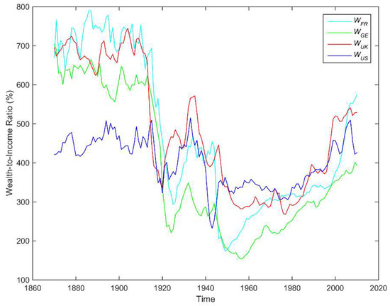
Figure 1.
The annual series of wealth-to-income ratio of the four countries covering the period 1870–2010.
The economic insights with regard to the selection of the dataset of wealth-to-income ratios are the following: a comparative analysis of the lead-lag relationships of private wealth-to-income ratios between four developed economies enhances our understanding about the underlying dependencies of these economies. The long-term evolution of the wealth-to-income ratio has implications to both the economic and the financial sector of a country (World Inequality Report 2018). In addition, the detection of leading indicators at cross-country level is useful as the latter are frequently employed as auxiliary forecasting tools in econometric models for cross-country economic studies (Moore 1975). The results of the paper shed light on the dynamic nature of the relationship between the wealth-to-income ratios of the four countries; they reveal changes in leadership in the short-run but static structures of leadership in the long-run. The evidence from such a study is innovative as no other study, to the best of our knowledge, focuses on this research question.
In addition, other advantages resulting from the selection of this dataset is that the dataset is open source, publicly available and reproductible. Thus, validation and/or extension of the current paperwork can be easily performed. As this is the first study, to our knowledge, that applies a comparison of two different methodological concepts for the detection of lead-lag relations, a dataset of annual time-series without complexity, such as seasonality or sensitivity due to high frequency variations, is considered as appropriate for the purpose of the demonstration of the comparison as well as for the interpretation of the findings.
4. Methodology
4.1. Time Domain Analysis
In order to investigate the pairwise lead-lag relationships between the wealth-to-income ratios of the countries using a time domain methodology, a bivariate econometric approach is employed. Let and be two time-series representing the wealth-to-income ratio , of two countries . For every pair of and included in the dataset, the following methodological steps are applied:
- Investigation of the stationarity of and to determine the order of integration of the variables.
- Specification of the lag order to include in the cointegration analysis.
- Investigation of the cointegrating relationship between and .
- Estimation of the coefficients of the VEC model in order to determine the lead-lag relationship between and .
Stationarity Test. The first step of the time domain methodology is to check the stationarity of the time-series. The Augmented Dickey–Fuller (ADF) unit-root test (Dickey and Fuller 1979) is performed on the original time series and on the time-series where is the first-order difference operator. The same procedure is followed for the time-series . For the ADF test, the null hypothesis is that contains a unit root or equivalently the time-series is non-stationary and the alternative is that was generated by a stationary process. In fact, the ADF test assumes that the series follows an AR() process where is the number of lagged difference terms of the variable in the regression. As the usual practice when performing the ADF test, in order to remove serial correlation in the residuals of the regression, whereas in case of the test corresponds to the standard (simple) Dickey-Fuller test. The t-statistic is used to test and finally the p-value for the test of against is reported.
The result of the stationarity test is important as it determines latter the choice of the bivariate time-series analysis model to be used; either a VAR model or a VEC model. A VAR model is selected in case that both time-series are integrated of order (denoted as ) whereas a VEC model is selected in case that the time-series are integrated of order (denoted as ) and there is evidence of cointegration among the series. The rest of the methodology sections continues with the regards to the case that both and are variables as this is the case of the time-series of the paper’s dataset based on the stationarity results.
Selection of optimal lag order. Before testing for co-integration or before fitting a VEC model, the optimal number of lags, also known as lag order or lag length, should be specified for the pair of and . The selection of optimal lag order requires attention because inference based on multivariate model is dependent on its correctness (Hacker and Hatemi-J 2008). The optimal lag order is decided based on the following three information criteria: the Final Prediction Error criterion (FPE) (Ljung 1999), the Akaike’s information criterion (AIC) (Akaike 1973) and the Hannan and Quinn information criterion (HQIC) (Hannan and Quinn 1979). As suggested by (Nielsen 2006), these lag-order selection methods can be employed in case of variables. According to each one of the criteria, the optimal model is selected as the one that minimizes the following score correspondingly:
where is the sample size (i.e., the number of observations), is the vector of predition errors, are the estimated parameters, is the number of estimated parameters in the model and is the maximized log-likelihood of the model. Given the results of the above three scores, the optimal lag order is selected as the number of lags suggested by the majority of the information criteria.
Testing for cointegration. The purpose of this step is to determine whether the pair of the series and are cointegrated or not. In case of cointegration, the number of cointegrating vectors existing between the variables is also computed. According to Engle and Granger (1987), a linear combination of two or more non-stationary time-series may be stationary. The definition of a bivariate cointegrating relation requires that there exist a linear combination of the variables that is . More specifically, if there are two parameters and , , such that is , then and are cointegrated meaning that they move together in the long-run. If such a stationary linear combination exists, this combination, known as the co-integrating equation, is interpreted as a long-run equilibrium relationship among the variables. If is a vector of variables, i.e., for a set of variables, the parameters and constitute the cointegrating vector , such that is a vector of variables.
Let consider a VAR process with lagged terms, denoted as VAR():
where are matrices of parameters, is a vector of constants (also known as intercepts) and is vector of error. Then, we may rewrite the VAR in the form of a VEC model:
where , , v and remain as in (4). It worth noting that a VEC() model can be converted to a VAR() model in levels with . For definitions, the term “lag order” in this paper refers to the order of the underlying VAR.
According to (Engle and Granger 1987), if all variables in are , the matrix has rank , where is the number of cointegrating relations. Regarding (also known as cointegrating rank), there are the following cases:
- If , there is no cointegration among the non-stationary variables and a VAR in their first differences is consistent.
- If , all the variables in are and a VAR in their levels is consistent.
- If then can be expressed as where and are matrices of rank .
The cointegration rank shows the number of cointegrating vectors. For instance, a rank of indicates that one linearly independent combination of the non-stationary variables and is stationary.
There are several different frameworks for estimation and inference in cointegrating systems. The paper of (Maddala and Kim 1998) surveys all these methods. In this study, for determining the number of co-integration relationships , the Johansen’s method (Johansen 1995) is employed as this method is recommended by several comparative studies including (Gonzalo 1994) and (Hubrich et al. 2001). According to (Johansen 1995), the null hypothesis is that there are no more than cointegrating relations. The Johansen’s maximum likelihood estimator of the parameters of the cointegrating VEC and two likelihood-ratio (LR) tests are applied for inference on . These LR tests are known as the trace statistic and the maximum-eigenvalue statistic because the log likelihood can be written as the log of the determinant of a matrix plus a simple function of the eigenvalues of another matrix. Let be the eigenvalues used in computing the log likelihood at the optimum. Johansen’s testing procedure starts with the test for zero cointegrating equations (i.e., a maximum rank of zero) and then accepts the first null hypothesis that is not rejected. By using the null hypothesis and restricting the number of cointegrating equations to be or less implies that the remaining eigenvalues are zero. According to (Johansen et al. 2000), the trace statistic is:
where is the number of observations and the are the estimated eigenvalues. For any given value of , large values of the trace statistic are evidence against the null hypothesis that there are or fewer cointegrating relations in the VEC model. The rest of the methodology sections continues under the assumption both and are and cointegrated as this is the case of the time-series of the paper’s dataset based on the results of stationarity and cointegration tests. Thus, a VEC model, rather than a VAR model, is to be fitted to the time-series during the next methodological step.
Estimation of the coefficients of the VEC model. Having determined that and are cointegrated, the next step is to estimate the parameters of a bivariate VEC model for the two series. The VEC model restricts the long-run behavior of the endogenous variables to converge to their cointegrating relationships while allowing for short-run adjustment dynamics. The cointegration term is known as the error correction term since the deviation from long-run equilibrium is corrected gradually through a series of partial short-run adjustments. The following part of the methodology assumes that there exists cointegrating relationships between the variables of and thus can be expressed as . The Equation (5) can be rewritten as:
The parameters of interest in the above VEC model are:
- the parameters of the cointegrating matrix ,
- the parameters of the adjustment matrix and
- the parameters of the short-run coefficient matrix .
In the case of a bivariate VEC with cointegrating equation, and are vectors, that is , and is matrix given by
Based on the Equation (7), we express the individual variables and as follows:
where
is the error correction term lagged one period (also known as the cointegration term).
An interpretation of the parameters of interest is given as follows. According to the theory of the VEC model, the parameters of the cointegrating vector show the long-run equilibrium relationships between levels of variables. In other words, contains the cointegrating relationship which represents the linear combination of and . Considering the definition of the cointegration:
the parameters that to be estimated are two. However, if is , so is for any finite, nonzero, real number . Thus, a normalization is performed and the coefficient of in (11) is unity. If and deviate from the long-run equilibrium, the error correction term will be nonzero and each variable adjusts to partially restore the equilibrium relation. The coefficients , also known as loading coefficients, measure how and react to deviations from the long-run equilibrium. In other words, they measure the speed of adjustment of the endogenous variable and correspondingly towards the equilibrium; the greater the coefficient, the higher speed of adjustment of the model from the short-run to the long-run. Finally, the parameters of the matrix show the short-run changes occurring due to previous changes in the variables.
The lead-lag relationship between the two variables is decided based on the values of the coefficients of the Equations (8) and (9). The following cases are possible:
- If the coefficients are non-zero or the error correction coefficient has a significant value, there is some information in that will be assimilated in later values of ; meaning that leads . More specifically:
- ○
- The existence of non-zero and significant coefficients in (8), i.e., the lagged coefficients of in the regression of indicate that there is a short-run causality between and : causes .
- ○
- The existence of a significant error correction coefficient indicates that there is a long-run causality between and : causes .
- If the coefficients are non-zero or the error correction coefficient has a significant value, there is some information in that will be assimilated in later values of ; meaning that leads . More specifically:
- ○
- The existence of non-zero and significant coefficients in (9), i.e., the lagged coefficients of in the regression of , indicates a short-term causality; causes .
- ○
- The existence of a significant error correction coefficient indicates that there is a long-run causality; causes .
- If all coefficients , , , have significant values, there is a two-directional relationship between the variables and .
4.2. Wavelet Analysis
In this part of the methodology, the wavelet concept is used to characterize how the relationship of two time-series evolves over time. More specifically, the continuous cross-wavelet transform is used to investigate the evolution of covariance of two time-series and the phase analysis of the wavelet coherence is employed to characterize the co-movement of the two series in the time-frequency domain. In the bibliography, there are many wavelet functions that one may choose from and many more that can be designed. In this paper, the Morlet wavelet function (also known as Gabor wavelet) is used as it is frequently employed in economic and financial studies to study the dynamic relationship of a pair of variables. In the following paragraphs, the concept of wavelet transform is briefly presented.
The basic Morlet wavelet function (also called mother wavelet), which can be seen as a Gaussian modulated harmonic function, is defined as:
where is a non-dimensional frequency and is a measure of the spread or support and satisfies the condition and . Traditionally, the parameters and are defined as (Strang and Nguyen 1997): and . This is the basic wavelet function and based on it, a family of wavelet functions can be constructed by varying the wavelet scale and translating along the time axis, as follows:
where is a normalization constant that guarantees that the wavelet has unit variance and where and are the translation (localization) and scale parameters that determine the exact position of the wavelet and wavelet dilution correspondingly. The scaling factor controls the wavelet’s width and the translation parameter controls the wavelet location (sliding) in the time axis.
The Morlet wavelet transformation for a time-series at scale and translation is defined:
where denotes the complex conjugate of the Morlet wavelet . In addition, the wavelet power spectrum is given by and can be interpreted as a measure of the local variance for the series at each time scale.
The cross-wavelet transform of two time-series, and , is defined as follows:
where and are the Morlet wavelet transformation of the time-series and respectively and denotes the complex conjugate. Τhe cross-wavelet spectrum is given by and can be interpreted as the local covariance of the two series at each time and frequency.
The complex wavelet coherency is defined as follows:
where represents a smoothing operator for both time and scale.
The wavelet coherence is the absolute value of the complex wavelet coherence and is given by:
resembles the correlation coefficient with low values providing evidence of weak correlation between two time-series and high values indicating strong correlation between two time-series. The wavelet coherence allows for a three-dimensional analysis, considering the time and frequency components as well as the strength of correlation. Thus, the wavelet coherence allows the detection of local correlation between the two series, the identification of structural changes over time as well as the short-run and long-run relations across frequencies. The theoretical distribution of the wavelet coherence is unknown, so statistical significance of its values is obtained using Monte Carlo procedures (Torrence and Compo 1998). Considering the Equation (17), the wavelet coherence is a positive value, so we cannot distinguish between positive and negative correlation. However, the phase difference, between two time-series is used to capture positive or negative correlation and the lead-lag relationships between the two time-series in the time-frequency space. In the polar form, the complex wavelet coherence can be expressed as .
The wavelet coherence phase difference (or phase angle) is the angle of the complex wavelet coherence and is defined as:
where and are the imaginary and real part of the smooth power spectrum respectively. We distinguish the following cases (Tiwari et al. 2013):
Phase difference between two time-series are indicated in the wavelet coherence plots by means of arrows. Here is a short description of the notation of the phase arrows. Arrows pointing to the right indicate that and move in-phase (analogous to positive correlation); arrows to the right and up mean that is leading whereas arrows to the right and down mean that is leading. Arrows pointing to the left indicate that and move anti-phase (analogous to negative correlation); arrows to the left and up mean that is leading whereas arrows to the left and down mean that is leading.
5. Empirical Results
This section presents the results of the application of the above described methodologies to the dataset. Initially, the empirical evidence using the time domain methodology is presented and the results of the wavelet analysis follow. A discussion on the consistency and on the complementarity of the two approaches is presented at the end of the section.
5.1. Time Domain Analysis
The results of the ADF unit root tests are reported in Table 2. A series of tests was performed for the variables , , , as well as their first difference and the number of autoregressive lags ranged in in order to determine the order of integration. The critical values of the t-statistic based on the tables in Fuller (1996) are −2.577 (10% critical value), −2.887 (5% critical value) and −3.497 (1% critical value). Statistically significant values of the t-statistic are indicated at *** 99% confidence, ** 95% confidence or * 90% confidence in Table 2. The decision of inclusion of trend and/or intercept in the implementation of the ADF test, involved a combination of theory and visual inspection of the data. There is no evidence in the bibliography that the ratio of wealth-to-income favors a particular null hypothesis in order to choose trend and/or intercept based on that. In addition, the data do not show a clear upward trend over the period of years 1870–2010. Thus, the ADF tests performed did not include intercept and linear time trend.
Table 2.
Results of unit root tests.
For all four countries, the ADF test indicates that the null hypothesis, regarding the presence of a unit root, is rejected for the original time-series (, , and ). Thus, the series are non-stationary at level. When the ADF test is performed on the first differences of the series (, , and ), there is evidence of stationarity. Thus, we consider that all the original series are integrated of the same order, i.e., . The same conclusion is retrieved when performing ADF tests including linear trend and/or intercept.
In the next step, the selection of appropriate lag length has been performed. Table 3 presents the scores of the three information criteria (FPE, AIC and HQIC) in terms of different lag orders () for each pair of variables. The minimum values for each criterion is indicated by “*”.
Table 3.
Score results of the criteria for lag order selection regarding the pairs of variables: , , , , and .
As determined by the most of the information criteria, the optimal lag order for the pair is 3, for the pair is 4, for the pair is 3, for the pair is 3, for the pair is 3 and for the pair is 4. The above mentioned lag orders are used for the cointegration analysis and for the fitting of the bivariate VEC models.
Following, the cointegration for each pair of variables has been tested using the Johansen’s trace. The results of these tests are shown in the Table 4. The first column of the Table 4 is the maximum rank, i.e., number of cointegrating relationships, used in the null hypothesis of the Johansen’s testing procedure. The rest columns present the trace statistic for each pair of variables in the dataset. The statistically significant values of the trace statistic are indicated by “*”. For the tests, the 5% critical value of the trace statistic is 15.41 for maximum rank = 0 and 3.76 for maximum rank = 1.
Table 4.
Results of the Johansen’s tests for cointegration.
For example, regarding the relationship between , the trace statistic at maximum rank = 0 equals 16.4989 which exceeds its critical value of 15.41, thus, we reject the null hypothesis of no cointegrating equations. In contrast, when testing for maximum rank = 1, equals 1.8499 which is less than its critical value of 3.76, so, we cannot reject the null hypothesis that there at most 1 cointegrating equation. As Johansen’s method for estimating the maximum rank accepts the first rank for which the null hypothesis is not rejected, we accept that the rank equals 1 for . Based on the results of the cointegration tests and considering the rest pairs of variables, we conclude that there is one cointegrating equation for every pair. Thus, each pair of variables has a long-run equilibrium relationship. However, in the short-run there may be deviations from this equilibrium and the error correction mechanism of a VEC model provides a means to reconcile the short-run and the long-run behavior.
The estimated coefficients of the bivariate cointegrating VEC models are presented in the Table 5, Table 6, Table 7, Table 8, Table 9 and Table 10 for each pair of variables respectively. As an example, the description and interpretation of the VEC model between and is analyzed following. The estimated parameters of this cointegrating VEC model is presented in Table 6. Table 6 contains the estimates of the short-run coefficients , the estimates of the error correction parameters and the constant , along with their standard errors presented in parenthesis. The second (lower) part of Table 6 presents the estimated parameters of the cointegrating vector for this model; also here the standard errors are shown in parenthesis. Statistically significant parameters are indicated at *** 99% confidence, ** 95% confidence or * 90% confidence. Based on Table 6, the dynamics of the short-run and the long-run relationship between and are analyzed as follows. In the equation of , the existence of a statistically significant coefficient of the error correction term indicates the existence of a long-run causality between and . This causality is running from to . In other words, the changes in can be explained by the changes in . The negative sign of the coefficient represents the negative feedback necessary when is too high to bring it back towards the levels. The absolute value of the estimated coefficient of the error correction term indicates the rate of convergence to the equilibrium per year. More precisely, the speed of adjustment of any disequilibrium towards the long-run equilibrium is that 13.52% of the disequilibrium is corrected each year. As expected, the adjustment parameters and have adverse signs indicating the two adjustment directions towards the equilibrium. In the equation of , the positive loading coefficient implies that when the value of is too high, the adjusts toward at the same time that is adjusted. Regarding the estimated cointegrating equation, there is the normalized coefficient of unity on and an estimated coefficient of −1.2154 on and it is significantly different from zero. Thus, we can conclude that the linear combination is a variable in the long-run. It worth noting that the significance of the coefficient of the lagged error correction term and the significant coefficient estimated in the cointegrating equation indicates that a VAR model in first differences of the variables would result in inconsistent estimates. Finally, regarding the short-run relationship between the variables, the estimated coefficients of lagged one period in the equation are statistically significant at 90% confidence level indicating the presence of a short-run causality from to .
Table 5.
The estimates of the parameters of the bivariate cointegrating VEC model for the series of and (upper part) and of the cointegrating equation for this model (lower part).
Table 6.
The estimates of the parameters resulted from the bivariate cointegrating VEC model for the series of and .
Table 7.
The estimates of the parameters resulted from the bivariate cointegrating VEC model for the series of and .
Table 8.
The estimates of the parameters resulted from the bivariate cointegrating VEC model for the series of and .
Table 9.
The estimates of the parameters resulted from the bivariate cointegrating VEC model for the series of and .
Table 10.
The estimates of the parameters resulted from the bivariate cointegrating VEC model for the series of and .
Regarding the long-run relationships, Table 5, Table 6, Table 7, Table 8, Table 9 and Table 10 show that the cointegration equations for all pairs of the studied variables are highly significant at 99% confidence. The long-run relationship for is estimated as (1, −0.9848) with speed of adjustment −0.1220, for is estimated as (1, −1.2154) with speed of adjustment −0.1352, for is estimated as (1, −1.1670) with speed of adjustment −0.0460, for is estimated as (1, −0.8119) with speed of adjustment −0.0628, for is estimated as (1, −0.9265) with speed of adjustment −0.0188 and for is estimated as (1, −1.1875) with speed of adjustment −0.0294. The negative and statistically significant value of the error correction term (99% confidence for the first 4 relationships and 90% confidence for the latter 2 relationships) indicates the existence of a long-run causality between the pairs of variables. More specifically, the results provide evidence that in the long-run leads both and , leads , leads the variables of , and . In addition, the estimated cointegration for and exhibits the largest error correction mechanism (−0.1352).
Regarding the short-run relationships and according to the results of Table 5, Table 6, Table 7, Table 8, Table 9 and Table 10, there is a unidirectional short-run causality running from to as indicated by the coefficient in the equation of , there exists a bidirectional (two-way feedback) relationship between and and a bidirectional relationship between and as well.
5.2. Wavelet Analysis
This subsection presents the results obtained by the application of the wavelet analysis. The computation of the wavelet spectrum of the uni-variate case (namely, the wavelet spectrum of the wealth-to-income ratio of each one of the four countries) and the bi-variate case (namely, the cross-wavelet spectrum for every pair of wealth-to-income ratio), as well as the wavelet phase angle values has been carried out in MATLAB using the “wavelet coherence toolbox”cdescribed in (Grinsted et al. 2004). The source code of this toolbox is open source, freely available under the MIT copyright license and can be found in the webpage of (Grinsted 2014).
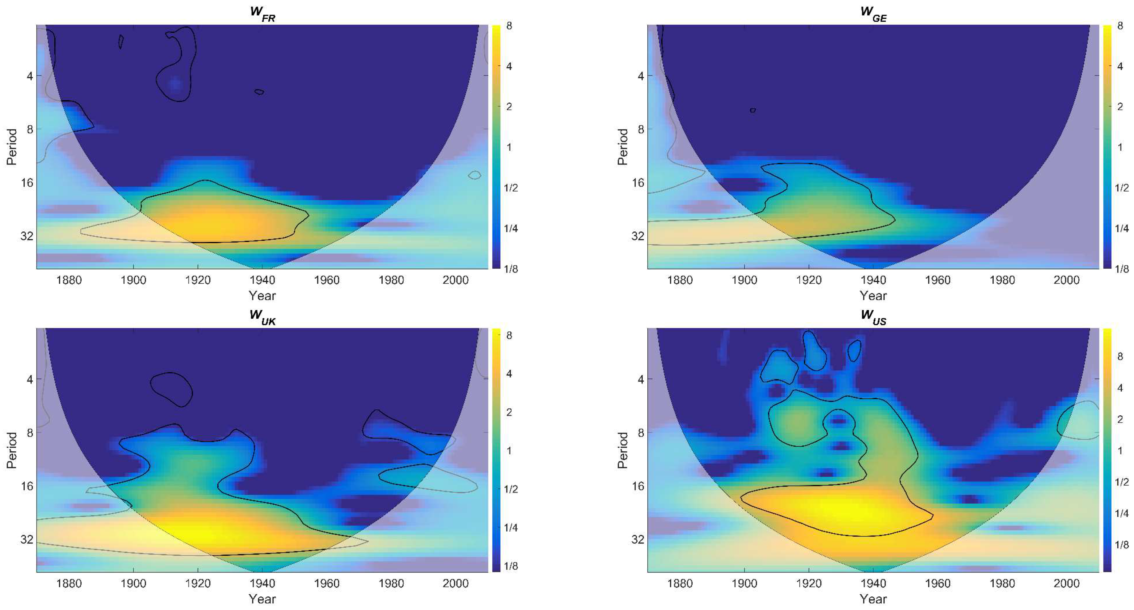
Figure 2 presents the wavelet power spectrum of , , and respectively. Although, the individual wavelet power spectrums do not bear any information for the lead-lag relationships between the pairs of the variables, they are presented as they form the basis for the wavelet coherence (WTC). In all plots of Figure 2, the time dimension is displayed on the horizontal axis and the frequency dimension, i.e., period cycles, is presented on the vertical axis. The frequency is classified into four bands: 1–4, 4–8, 8–16 and 16–32 years frequency bands. These frequency bands can be described as short-run, medium-run, long-run and very long-run periods (Chen 2016). The power is presented by color, ranging from the blue (low power) to yellow (high power). As the time-series are of finite length, errors may occur at the beginning and end of the wavelet power spectrum; the cone of influence (COI), shown with thick black lines, indicates the region affected by the edge effects. As the results outside the COI region may not be reliable (Aguiar-Conraria and Soares 2014), this study focuses only on the wavelet power spectrums included in the COI. Regarding the significance levels of the wavelet power spectrum, the null hypothesis is defined as follows: it is assumed that the time series has a mean power spectrum; if a peak in the wavelet power spectrum is significantly above this background spectrum, then it can be assumed to be a true feature with a certain percent confidence. For definitions, “significant at the 5% level” is equivalent to “the 95% confidence level” and implies a test against a certain background level, while the “95% confidence interval” refers to the range of confidence about a given value. The thick contoured closed regions in the plots of Figure 2 indicate the 95% confidence level for the corresponding spectrum. For example, in Figure 2, the 95% confidence level for is shown by the thick contour indicating that during 1900–1950 the variance in the 16–32 year band is significant at 95% confidence level. Regarding , a similar result is presented during 1900–1940. For and , the variance shows a gradual increase with period, primarily during 1900–1970 and there are a few isolated significant regions around the cycle of 4 years. In all plots of Figure 2, the significant volatilities at difference frequency bands identified over various periods suggest that WWII is likely to have influenced the wealth-to-income ratio in all ranges of frequency bands (from short to very long-run) in all four countries.
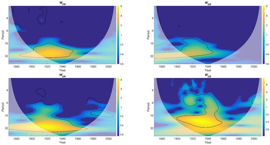
Figure 2.
The decomposition in the time and frequency domain for the time-series of wealth-to-income ratio of the four countries.
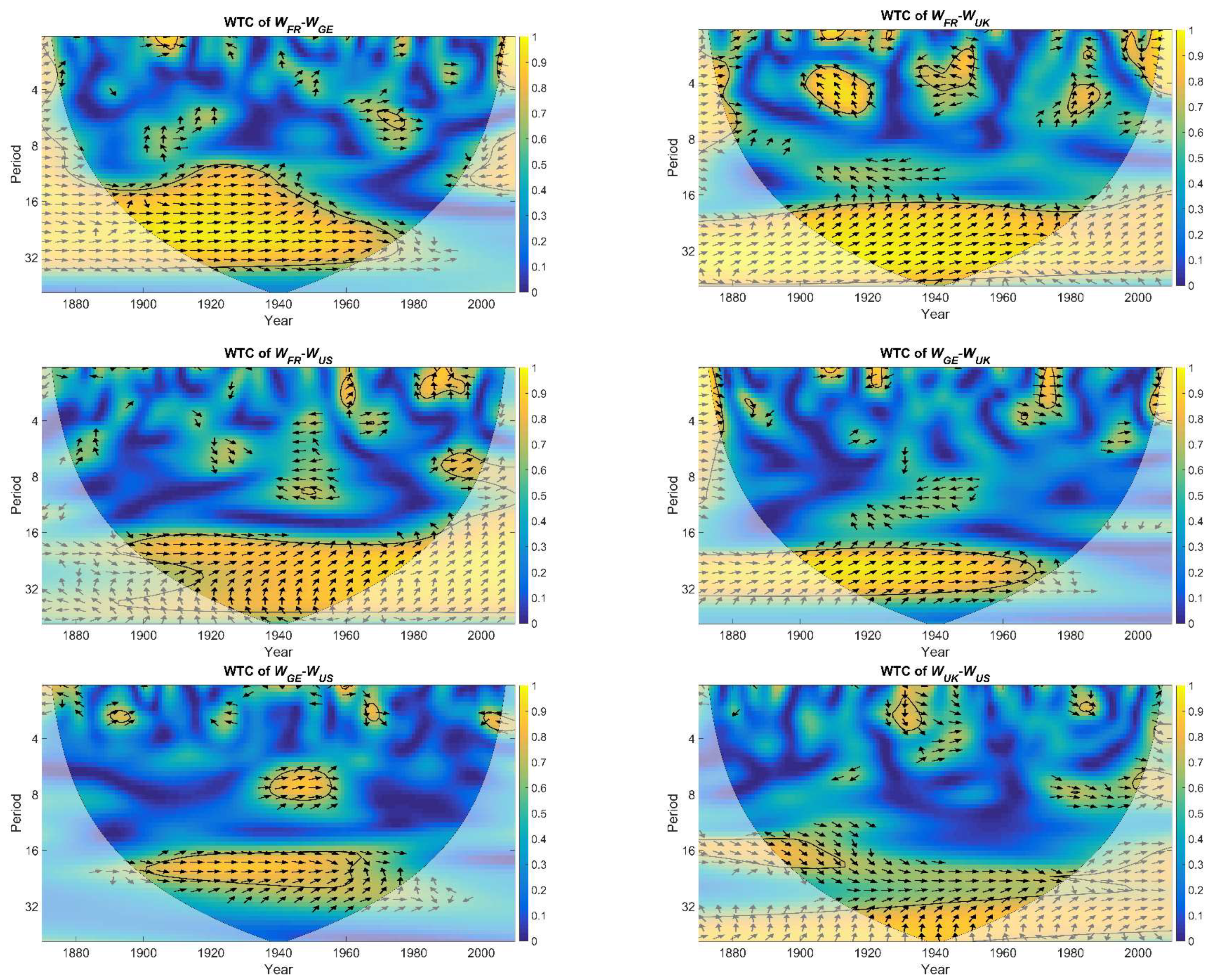
In order to investigate the pairwise lead-lag relationships between the four studied variables, Figure 3 presents the WTC between all the pairs of the studied variables. As the wavelet coherence finds regions in the time-frequency plane where the time-series co-vary, there are high correlations at 5% significant level in the 16–32 year band during the period 1900–1960. Considering that there exists one value of the wavelet phase difference for every combination of time point (year in the x-axis) and frequency band (point in the y-axis), the arrows in Figure 3 represent a subset of the values of the phase angle across blocks of years and across blocks of frequency bands. This representation is performed for visualization purposes and in addition, only values of wavelet phase difference where the underlying wavelet coherence is are presented. The cross-wavelet transform between and and between and are analyzed following as examples and the dynamics of the significant lead-lad relationships between all variables of the study are summarized in Table 11. Regarding the first example, Figure 3 demonstrates that and move in-phase (i.e., the phase difference approximately equals ) in the long-run and in the very-long run and leads . An isolated significant cluster around 1970 at the frequency band of 4–8 years indicates a significant positive (in-phase) relationship between the and which may be related to the historical fact of the creation of the European Economic Community in 1969. Regarding the second example pair, the four largest clusters of significant correlations indicate the following cases; and move anti-phase in the short-run around 1915 and around 1945 (i.e., around WWI and WWII respectively) where leads , they move in-phase in the medium-run around 1980 where leads , and they move in-phase where leads in the very long-run.
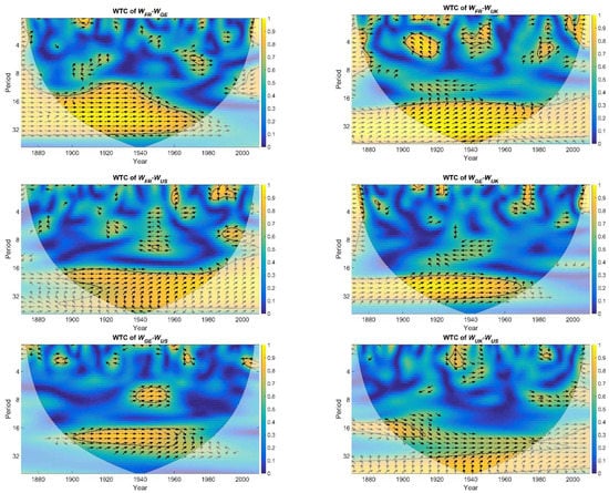
Figure 3.
The wavelet coherence and the phase difference for every pair of wealth-to-income ratio.
Table 11.
Presentation of the lead-lag relationships for all pairs of the studied variables based on the phase angle difference of the wavelet coherence.
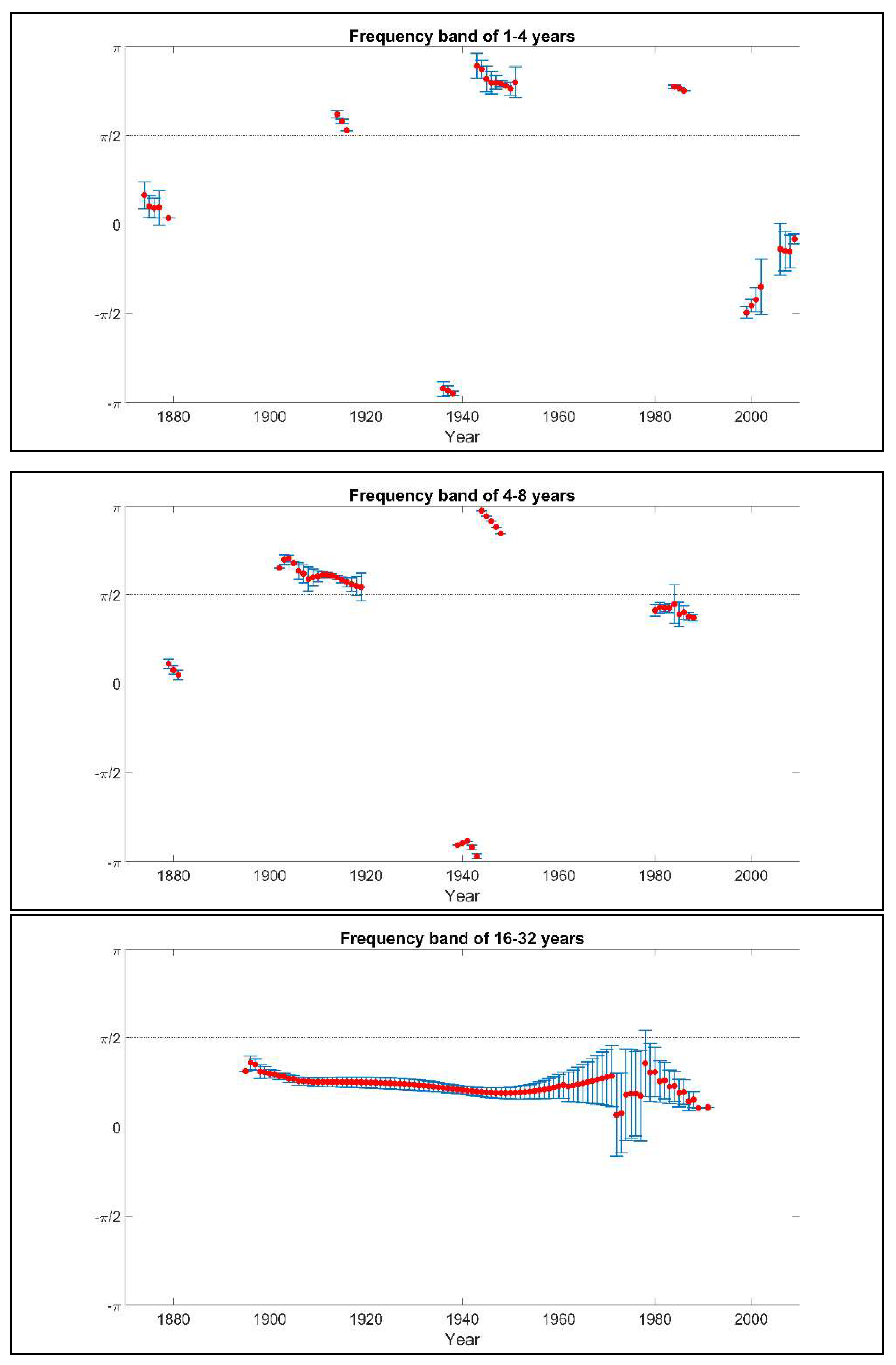
In order to obtain a detailed representation of phase angle values and in order to reduce the complexity in its representation, it is useful to derive the tendency in the relationship between the series in the time dimension and scale dimension. For that purpose, based on the calculation of the wavelet phase difference for every combination of time point (year) and frequency point (frequency band), we focused on the statistically significant values of phase angle and then we averaged the phase angle values over time separately for each frequency band. Due to space limitations, we show in detail only the case of the plots of the phase angle for the pair of and in Figure 4. Figure 4 includes three plots of the phase angle for the frequency band 1–4 years, 4–8 years and 16–32 years respectively; the frequency band of 8–16 years includes no statistically significant phase angle values. For example, in the medium-run leads in the periods 1902–1920 and 1945–1948 whereas leads in the periods 1879–1881, 1939–1943 and 1980–1988. The lead-lag results derived from the detailed analysis of the phase angle for the above-mentioned pair and for the rest pairs of the study are presented in Table 11. In Table 11, a lead-lag relationship is described in terms of a specific timescale (frequency band), a specific time period (indicating by starting and ending year) and the leading variable. The correlation between the variables, either positive (in-phase) or negative (anti-phase) is also presented in parenthesis. The results indicate that the leading variable in all relationships is not static over time but it is differentiated depending on the period and on the timescale. In the very long-run, the conclusions driven by the wavelet analysis are that leads , that leads both and , and that leads , and .
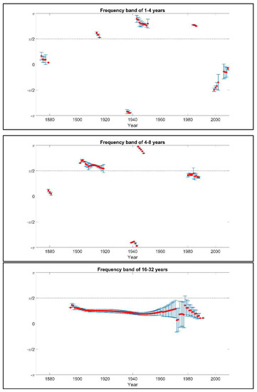
Figure 4.
Plot of the phase angle of the wavelet coherence between and for the three frequency bands respectively; 1–4 years (up), 4–8 years (middle), 16–32 years (down). Red dots represent the averaged phase angle over time and blue lines represent the corresponding variance.
Table 11 summarizes the lead-lag relationships between the six studied relationships where only the periods of significant correlation are presented. The relationship of each pair of variables is captured in terms of a specific timescale and the leading variable is indicated. The correlation between the two variables, either positive (in-phase) or negative (anti-phase), is presented in parenthesis. The results indicate that the leading variable in all relationships is not static over time and it is differentiated depending on the period and on the timescale. In the timescale of 16–32 years, the conclusions driven by the wavelet analysis are that leads , that leads both and , and that leads , and .
5.3. Comparison of the Two Methodologies
To uncover the behavior of the lead-lag relationship between pairs of time-series two different concepts are employed. The fitting of a VEC model to the non-stationary but cointegrated series provides evidence of both the short-run relation and existence of a long-run equilibrium relation between the independent and dependent variable. In addition, the model computes the speed of adjustment of any disequilibrium towards the long-run equilibrium; it can also be seen as the rate of convergence to the equilibrium state per time cycle (i.e., per year in case of annual time-series). On the other hand, the computation of the phase angle of wavelet coherence offers two main advantages; first, it uncovers the dynamic patterns between the variables by allowing for time-varying leadership between the independent and dependent variable and second, it decomposes the lead-lag relationship over various time horizons. In order to compare the time horizon of the long-run equilibrium of the VEC model to the timescales of the wavelet analysis, we consider that the long-run equilibrium of the first methodology corresponds to the timescale of 16–32 years of the second methodology. In the following, the term long-run refers to the long-run equilibrium of the VEC model.
The application of the methodologies to the wealth-to-income ratios of four developed economies yields several important results. First, the long-run results of the two methodologies are consistent, i.e., leads , that leads both and , and that leads , and . Regarding the series of and , for example, both methods confirm the leadership of towards in the long-run. The VEC model provides evidence that the linear combination is an variable in the long-run with speed of adjustment −0.1352 and this result is significant at the 95% confidence level. The coefficient of the error correction term in the equation has a statistically significant and negative value indicating that causality runs from to . The examination of the causal relationship between based on the phase angle statistics reveals that leads over the period 1889 – 1968 in the timescale of 16–32 years and this result is significant at the 95% confidence level. When comparing the short-run results derived from the two methodologies, the VEC model detects a short-run causality from to as the lagged one period coefficients of is statistically significant at 90% level of significance in the equation. From the wavelet perspective of analysis, a causality from to is detected over the period 1970–1977 in the timescale of 4–8 years. Table 12 presents a comparative summary of the main statistically significant findings of the two methodologies; regarding the time domain methodology the long-run and the short-run results (if any) are presented and regarding the time-frequency domain methodology the results in terms of the long-run, the short-run and the medium-run are summarized. Table 12 as well as the detailed results of the two methodologies presented in Section 5.1 and Section 5.2 suggest that the lead-lag relationship between two time-series is best uncovered using methods both from the time and from the time-frequency domain. The contribution of the phase angle analysis of wavelet coherence is especially useful in cases where an altering in leadership takes place over time; an example is the relationship between where in the timescale of 4–8 years leads in 1902–1920 and 1945–1948 whereas leads in 1879–1881, 1939–1943 and 1980–1988. Thus, we conclude that the two methodologies bear complementary information regarding the relationship of the variables and the use of both a time domain and a time-frequency domain approach provides a more detailed understanding in the context of time-varying lead-lag effects.
Table 12.
Main findings of the two methodologies regarding the lead-lag relationships for all pairs of the studied variables.
6. Conclusions
In this article, the detection of lead-lag relationships in economic time-series is addressed by the joint application of two conceptually different methodologies. Even though, the research question of lead-lag relationships has been examined in a large number of studies using either a time domain method or a time-frequency domain method, this article enriches the existing literature by presenting a joint application of the two methods on a dataset and by providing a detailed comparison of their results. Based on the joint application of the two frameworks, the question of their consistency and their potential complementarity is addressed. This study provides empirical evidence about the consistency of the two methodologies in the short-run, in the log-run as well as about the dynamics of the lead-lag behavior over time. In addition, the study reveals that each methodology provides evidence on different aspects of the lead-lag relationships and suggests the complementarity of the results of the methods in the short-run. The results of the paper confirm that the joint application of the two studied methodologies results in a more informative understanding of the dynamic nature of lead-lag relationships over time.
More specifically, the VEC model is selected among the time domain methods as it suitable for the investigation of the relationship of non-stationary but co-integrated time-series. The phase angle of the wavelet is adopted among the methods of the time-frequency domain to demonstrate the dynamic nature of the lead-lag relationships over time and across various timescales. The VEC model provides the speed of adjustment from any disequilibrium to the long-run equilibrium, information which is not provided when using the wavelet analysis. In addition, the VEC model detects short-run causal relationships, which according to the theory of the model remain static all over the time-period of study. On the other hand, the wavelet analysis is able to demonstrate changes in leadership over time and in multiple time horizons such as the short-run, the medium-run and the long-run. This capability of the wavelet analysis is not provided when applying the VEC analysis.
The application of the two methodologies to the dataset of wealth-to-income ratios of the economies of France, Germany, UK and USA. With regards to the application of the methodologies to the dataset of wealth-to-income ratio, this paper contributes to the existing literature by providing new evidence on the lead-lag relationships of the wealth-to-income ratio of France, Germany, United Kingdom and the United States of America both in the long-run and in the short-run. The empirical country-by-country comparison of the private wealth-to-income ratios and the detection of lead-lag relationships among them enhances our understanding about the underlying dependencies of these economies. More specifically, the results of the study indicate that the main long-run findings of the two methods in terms of leadership are consistent; leads , that leads both and , and that leads , and . Further conclusions driven by the wavelet analysis regarding the short-run and medium-run perspective demonstrate changes in the leadership depending on the time period and indicate the dynamic nature of leadership between the variables. Overall, the combination of the two methodological concepts provides a more informative picture on the dynamics of the lead-lag relationship between two time-series compared to the results retrieved only by each one of the two methodologies.
Funding
This research received no external funding.
Acknowledgments
The author is grateful to the Professor of Finance Theoharry Grammatikos, University of Luxembourg, for his fruitful discussions during the preparation of this study. In addition, the author expresses gratitude to Christos Tsinos for his valuable recommendations on the wavelet methodology.
Conflicts of Interest
The author declares no conflict of interest.
References
- Afonso, António, Michael G. Arghyrou, George Bagdatoglou, and Alexandros Kontonikas. 2015. On the time-varying relationship between EMU sovereign spreads and their determinants. Economic Modelling 44: 363–71. [Google Scholar] [CrossRef]
- Aguiar-Conraria, Luís, and Maria Joana Soares. 2014. The continuous wavelet transform: Moving beyond uni and bivariate analysis. Journal of Economic Surveys 28: 344–75. [Google Scholar] [CrossRef]
- Ajayi, Richard A., and Mbodja Mougouė. 1996. On the dynamic relation between stock prices and exchange rates. Journal of Financial Research 19: 193–207. [Google Scholar] [CrossRef]
- Akaike, Hirotogu. 1973. Information theory as an extension of the maximum likelihood principle. In Second International Symposium on Information Theory. Budapest: Akademiai Kiado, pp. 267–81. [Google Scholar]
- Alzahrani, Mohammed, Mansur Masih, and Omar Al-Titi. 2014. Linear and non-linear Granger causality between oil spot and futures prices: A wavelet based test. Journal of International Money and Finance 48: 175–201. [Google Scholar]
- Baum, Christopher F. 2013. VAR. SVAR and VECM Models. EC 823: Applied Econometrics, Boston College, Spring 2013. Available online: http://fmwww.bc.edu/EC-C/S2013/823/EC823.S2013.nn10.slides.pdf (accessed on 14 March 2019).
- Bernoth, Kerstin, and Burcu Erdogan. 2012. Sovereign bond yield spreads: A time-varying coefficient approach. Journal of International Money and Finance 31: 639–56. [Google Scholar] [CrossRef]
- Campbell, John Y., Andrew W. Lo, and Archie Craig MacKinlay. 1997. The Econometrics of Financial Markets. Princeton: Princeton University Press. [Google Scholar]
- Chang, Chun-Ping, and Chien-Chiang Lee. 2015. Do oil spot and futures prices move together? Energy Economics 50: 379–90. [Google Scholar] [CrossRef]
- Chen, Wen-Yi. 2016. Health progress and economic growth in the USA: The continuous wavelet analysis. Empirical Economics 50: 831–55. [Google Scholar] [CrossRef]
- Chung, Pin J., and Donald J. Liu. 1994. Common stochastic trends in Pacific Rim stock markets. Quarterly Review of Economics and Finance 34: 241–59. [Google Scholar] [CrossRef]
- Cong, Rong-Gang, Yi-Ming Wei, Jian-Lin Jiao, and Ying Fan. 2008. Relationships between oil price shocks and stock market: An empirical analysis from China. Energy Policy 36: 3544–53. [Google Scholar] [CrossRef]
- Corhay, Albert, A. Tourani Rad, and Jean Pierre Urbain. 1993. Common stochastic trends in European stock markets. Economics Letters 42: 385–90. [Google Scholar] [CrossRef]
- Dickey, David A., and Wayne A. Fuller. 1979. Distribution of the estimators for autoregressive time series with a unit root. Journal of the American Statistical Association 74: 427–31. [Google Scholar]
- Engle, Robert F., and Clive W. J. Granger. 1987. Co-Integration and error correction: Representation, estimation, and testing. Econometrica 55: 251–76. [Google Scholar] [CrossRef]
- Estrella, Arturo, and Frederic S. Mishkin. 1998. Predicting U.S. recessions: Financial variables as leading indicators. Review of Economics and Statistics 80: 45–61. [Google Scholar] [CrossRef]
- Fuller, Wayne A. 1996. Introduction to Statistical Time Series, 2nd ed. New York: Wiley. [Google Scholar]
- Funashima, Yoshito. 2017. Time-varying leads and lags across frequencies using a continuous wavelet transform approach. Economic Modelling 60: 24–28. [Google Scholar] [CrossRef]
- Gençay, Ramazan, Faruk Selçuk, and Brandon J. Whitcher. 2002. An Introduction to Wavelets and Other Filtering Methods in Finance and Economics. San Diego: Academic Press. [Google Scholar]
- Gonzalo, Jesus. 1994. Five alternative methods of estimating long-run equilibrium relationships. Journal of Econometrics 60: 203–33. [Google Scholar] [CrossRef]
- Granger, Clive W. J. 1988. Some recent development in a concept of causality. Journal of Econometrics 39: 199–211. [Google Scholar] [CrossRef]
- Granger, Clive Wiliam John, and Oskar Morgenstern. 1970. The Predictability of Stock Market Prices. Lexington: Health Lexinghton Book. [Google Scholar]
- Grinsted, Aslak. 2014. Wavelet Toolbox by Grinsted. Available online: http://www.glaciology.net/wavelet-coherence (accessed on 14 March 2019).
- Grinsted, A., J. C. Moore, and S. Jevrejeva. 2004. Application of the cross wavelet transform and wavelet coherence to geophysical time series. Nonlinear Processes in Geophysics 11: 561–66. [Google Scholar] [CrossRef]
- Grossmann, Volker, and Thomas Michael Steger. 2016. Das House-Kapital: A theory of wealth-to-income ratios. In Annual Conference of Demographic Change 145936. Augsburg: German Economic Association. [Google Scholar]
- Gwilym, Owain Ap, and Mike Buckle. 2001. The lead-lag relationship between the FTSE100 stock index and its derivative contracts. Applied Financial Economics 11: 385–93. [Google Scholar] [CrossRef]
- Hacker, Scott R., and Abdulnasser Hatemi-J. 2008. Optimal lag-length choice in stable and unstable VAR models under situations of homoscedasticity and ARCH. Journal of Applied Statistics 35: 601–15. [Google Scholar] [CrossRef]
- Hannan, Edward J., and Barry G. Quinn. 1979. The Determination of the order of an autoregression. Journal of the Royal Statistical Society, Series B 41: 190–95. [Google Scholar] [CrossRef]
- Hoover, Kevin D. 2008. Causality in economics and econometrics. In The New Palgrave Dictionary of Economics, 2nd ed. Edited by Steven N. Durlauf and Lawrence E. Blume. New York: Palgrave Macmillan. [Google Scholar]
- Huang, Shupei, Haizhong An, Xiangyun Gao, and Xuan Huang. 2016. Time–frequency featured co-movement between the stock and prices of crude oil and gold. Physica A: Statistical Mechanics and Its Applications 444: 985–95. [Google Scholar] [CrossRef]
- Hubrich, Kirstin, Helmut Lütkepohl, and Pentti Saikkonen. 2001. A review of systems cointegration tests. Econometric Reviews 20: 247–318. [Google Scholar] [CrossRef]
- Jackline, Stella, and Malabika Deo. 2011. Lead-lag relationship between the futures and spot prices. Journal of Economics and International Finance 3: 424–27. [Google Scholar]
- Johansen, Søren. 1995. Likelihood-Based Inference in Cointegrated Vector Autoregressive Models. Oxford: Oxford University Press. [Google Scholar]
- Johansen, Søren, Rocco Mosconi, and Bent Nielsen. 2000. Cointegration analysis in the presence of structural breaks in the deterministic trend. Econometrics Journal 3: 216–49. [Google Scholar] [CrossRef]
- Kim, Sangbae, and Francis In. 2005. The relationship between stock returns and inflation: New evidence from wavelet analysis. Journal of Empirical Finance 12: 435–44. [Google Scholar] [CrossRef]
- Ko, Jun-Hyung, and Chang-Min Lee. 2015. International economic policy uncertainty and stock prices: Wavelet approach. Economics Letters 134: 118–22. [Google Scholar] [CrossRef]
- Koutmos, Gregory. 1996. Modelling the dynamic interdependence of major European stock markets. Journal of Business Finance & Accounting 23: 975–88. [Google Scholar]
- Ljung, Lennart. 1999. System Identification: Theory for the User, 2nd ed. Prentice-Hal PTR Information and System Sciences Series; Upper Saddle River: Prentice Hall. [Google Scholar]
- Maddala, Gangadharrao S., and In-Moo Kim. 1998. Unit Roots, Cointegration, and Structural Change. Cambridge: Cambridge University Press. [Google Scholar]
- Marczak, Martyna, and Thomas Beissinger. 2016. Bidirectional relationship between investor sentiment and excess returns: New evidence from the wavelet perspective. Applied Economics Letters 23: 1305–11. [Google Scholar] [CrossRef]
- Moore, Geoffrey H. 1975. Economic indicators and econometric models. Business Economics 10: 45–48. [Google Scholar]
- Nielsen, Bent. 2006. Order determination in general vector autoregressions. IMS Lecture Notes-Monograph Series, Time Series and Related Topics 52: 93–112. [Google Scholar]
- Nijman, Theo, and Frank de Jong. 1997. High frequency analysis of lead-lad relationships between financial markets. Journal of Empirical Finance 4: 259–77. [Google Scholar]
- Olayeni, Olaolu Richard. 2016. Causality in continuous wavelet transform without spectral matrix factorization: Theory and application. Computational Economics 47: 321–40. [Google Scholar] [CrossRef]
- Piketty, Thomas. 2014. Capital in the 21st Century. Cambridge: Harvard University Press. [Google Scholar]
- Piketty, Thomas, and Gabriel Zucman. 2014. Capital is back: Wealth-income ratios in rich countries 1700–2010. Quarterly Journal of Economics 129: 1255–310. [Google Scholar] [CrossRef]
- Piketty, Thomas, and Gabriel Zucman. 2015. Wealth and inheritance in the long run. Handbook of Income Distribution 2: 1303–68. [Google Scholar]
- Polanco-Martínez, Josué, and Luis Abadie. 2016. Analyzing crude oil spot price dynamics versus long term future prices: A wavelet analysis approach. Energies 9: 1089. [Google Scholar] [CrossRef]
- Polanco-Martínez, Josué Moises, Javier Fernández-Macho, Marc Neumann, and Sérgio Henrique Faria. 2018a. A pre-crisis vs. crisis analysis of peripheral EU stock markets by means of wavelet transform and a nonlinear causality test. Physica A: Statistical Mechanics and its Applications 490: 1211–27. [Google Scholar]
- Polanco-Martínez, Josué M., Luis M. Abadie, and Javier Fernández-Macho. 2018b. A multiresolution and multivariate analysis of the dynamic relationships between crude oil and petroleum-product prices. Applied Energy 228: 1550–60. [Google Scholar]
- Ramsey, James B. 1999. The contribution of wavelets to the analysis of economic and financial data. Philosophical Transactions of the Royal Society of London Series A 357: 2593–606. [Google Scholar] [CrossRef]
- Ramsey, James B. 2002. Wavelets in economics and finance: Past and future. Studies in Nonlinear Dynamics & Econometrics 6: 1–29. [Google Scholar]
- Ramsey, James B., and Camille Lampart. 1998. The decomposition of economic relationships by time scale using wavelets: Expenditure and income. Studies in Nonlinear Dynamics and Econometrics 3: 23–42. [Google Scholar] [CrossRef]
- Rault, Christophe, and Mohamed El Hedi Arouri. 2009. Oil Prices and Stock Markets: What Drives What in the Gulf Corporation Council Countries? Working Paper No. 960. Ann Arbor, MI, USA: William Davidson Institute. [Google Scholar]
- Reboredo, Juan C., and Miguel A. Rivera-Castro. 2013. A wavelet decomposition approach to crude oil price and exchange rate dependence. Economic Modelling 32: 42–57. [Google Scholar] [CrossRef]
- Reboredo, Juan C., Miguel A. Rivera-Castro, and Andrea Ugolini. 2017. Wavelet-based test of co-movement and causality between oil and renewable energy stock prices. Energy Economics 61: 241–52. [Google Scholar] [CrossRef]
- Rognlie, Matthew. 2015. Deciphering the fall and rise in the net capital share. Brookings Papers on Economic Activity 2015: 1–69. [Google Scholar] [CrossRef]
- Silvapulle, Param, and Imad A. Moosa. 1999. The relationship between spot and futures prices: Evidence from the crude oil, market. Journal Futures Markets 19: 175–93. [Google Scholar] [CrossRef]
- Stoll, Hans R., and Robert E. Whaley. 1990. Stock market structure and volatility. Review of Financial Studies 3: 37–71. [Google Scholar] [CrossRef]
- Strang, Gilbert, and Truong Nguyen. 1997. Wavelets and Filter Banks. Wellesley: Wellesley-Cambridge Press. [Google Scholar]
- Tiwari, Aviral Kumar, Mihai Mutascu, and Alin Marius Andries. 2013. Decomposing time-frequency relationship between producer price and consumer price indices in Romania through wavelet analysis. Economic Modelling 31: 151–59. [Google Scholar] [CrossRef]
- Toda, Hiro Y., and Peter C. B. Phillips. 1994. Vector autoregressions and causality: A theoretical overview and simulation study. Econometric Reviews 13: 259–85. [Google Scholar] [CrossRef]
- Tonn, Victor Lux, and Joseph McCarthy. 2010. Wavelet domain correlation between the futures prices of natural gas and oil. The Quarterly Review of Economics and Finance 50: 408–14. [Google Scholar] [CrossRef]
- Torrence, Christopher, and Gilbert P. Compo. 1998. A practical guide to wavelet analysis. Bulletin of American Meteorological Society 79: 61–78. [Google Scholar] [CrossRef]
- Visvikis, Ilias, Panayotis Alexakis, and Manolis G. Kavussanos. 2002. An investigation of the lead-lag relationship in returns and volatility between cash and stack index futures: The case of Greece. Paper presented at European Financial Management Association Annual Meeting, London, UK, June 26–29. [Google Scholar]
- WID Database. 2017. The World Wealth and Income Database. Available online: http://www.wid.world/#Database (accessed on 14 March 2019).
- World Inequality Report. 2018. Available online: https://wir2018.wid.world/part-3.html (accessed on 14 March 2019).
- Zavadska, Miroslava, Lucía Morales, and Joseph Coughlan. 2018. The lead-lag relationship between oil futures and spot prices—A literature review. International Journal of Financial Studies 6: 89. [Google Scholar] [CrossRef]

© 2019 by the author. Licensee MDPI, Basel, Switzerland. This article is an open access article distributed under the terms and conditions of the Creative Commons Attribution (CC BY) license (http://creativecommons.org/licenses/by/4.0/).