A Review of the Main Issues on the Loan Contracts: Asymmetric Information, Poor Transparency, and Hidden Costs

Abstract

The well-known subprime mortgage crisis, which began to manifest in early 2007, since when the effects of the speculative bubble begin to become evident from the increase in default rates in residential mortgages, has triggered a global crisis that has pushed various legislations over time to implement a series of financial reforms with the specific objective of avoiding that similar phenomena could be repeated over time. The ability to repay a loan is strongly influenced by the amortization algorithm that the bank has decided to adopt. This appears even more evident in variable interest rate loans since, as the economic conditions of the indexation parameter change, the definition of the loan balance and the related portion of interest will be decisive in relation to the borrower’s ability to repay the loaned capital. A study of the main amortization algorithms and the related descriptions in the bank contracts will allow us to show which are the main issues due to an information asymmetry that, unfortunately, characterizes this type of contract and would seem to be one of the main reasons that lie at the root of the aforementioned crisis of subprime mortgages in the USA. Moreover, the authors will provide a clear analysis of the financial indicators usually reported in loan contracts and how often these indications are insufficient to characterize the actual cost of the loan. Furthermore, by highlighting the discretionary choice that banks often obtain following the contractual loan schemes commonly offered to retail and corporate clients, we will show how this often translates into greater cost to the borrower. Finally, we will propose two possible solutions to the problems highlighted, thus allowing us to reduce this information gap, which unfortunately translates into greater costs for customers with the associated increase in default rates, or the so-called nonperforming loan (NPLs) contracts. Therefore, the objective of this contribution is to show which are the most critical aspects of the bank contracts related to contractual transparency and to the presence or otherwise of hidden costs, i.e., not expressly shown in the contract. Specifically, we refer to the loan contracts issued in Italy both with reference to the local banking legislation and to the European one to which Italy must often refer.

1. Introduction

The financial crisis has shown that irresponsible behavior by market operators can put the basics of the financial system at risk by creating a lack of trust between all the parties involved, in consumers in particular, and potentially serious socio-economic consequences. Many consumers have lost confidence in the financial sector and borrowers have found themselves increasingly struggling to meet their loans, which has led to an increase in the number of defaults and forced sales (Tang et al. 2008). When the bank pays a loan to a borrower, one of the main features that are the object of bargaining between the parties is the amortization schedule or the principal balance repayment algorithm that the bank proposes to the borrower for the repayment of the loaned capital and the related accrued interest. Some causes of these problems concern ineffective, inconsistent, or nonexistent regimes for credit intermediaries and noncredit institutions that provide credits for residential real estate. The problems identified may have significant cascading effects on the macroeconomic plan, causing harm consumers, acting as an economic or legal barrier to cross-border activities, and creating unequal conditions for market operators (Peng 2009). To this is added the presence of policies of poor transparency in the drafting of banking contracts with specific reference to the agreed amortization algorithm. Incorrect policies have been found by some financial operators who have offered consumers complex loan repayment algorithms that are not easily understood and that, in practice, have generated excessive borrowing for the borrower, often generating insolvencies or corporate defaults, which produce inevitable socioeconomic consequences. For this reason, specific attention must be given to the agreement of the loan amortization algorithm (Zhu and Yan 2013).

An amortization schedule is a table reporting each periodic payment of an amortizing loan according to the adopted algorithm. Amortization refers to the process of paying a debt through specific on-time payments. At each payment, the borrower pays a portion of interest while the remaining amount is computed towards the loaned principal balance. The percentage of interest versus principal is determined by the adopted amortization schedule. The adopted amortization algorithm schedule differentiates the portion of payment that belongs to interest from the portion used to repay the debt.

While a portion of every payment is applied towards both the interest and the principal balance of the loan, the exact amount applied to principal each time varies (with the remainder going to interest).

Due to the risk that the banks bear in relation to the nonrepayment (total or partial) of the loan granted, the latter performs accurate checks on potential borrowers, appropriately assessing the so-called credit risk. Multiple models for assessing credit risk and assessing customers (credit rating/scoring) have been proposed in the literature (Kellison 1970; Lasher 2008; Ross et al. 2000).

To the above, the risk of a legal action is added due to a nonexact correspondence between what is reported in the loan contract compared to what is actually applied by the credit institution in relation to the agreed amortization schedule. This kind of risk is linked to the so-called problem of “Asymmetric Contract Information” studied by some authors (Tian and Liu 2007).

Due to the aforementioned risks, legislation in various parts of the world has regulated the disbursement of loans and mortgages by banks in order to guarantee specific protection to both parties. With specific reference to the European continent, in relation to the protection of the borrower, the European community has issued several directives over time, the last of which is the Directive 2014/17/EU 2014 MCD (Mortgage Credit Directive), which arises the objective of giving greater protection to the borrower, as the aim is to guarantee a high level of protection for those who sign credit agreements relating to real estate (Directive 2014/17/EU 2014). More specifically, in this contribution we will refer to the banking contracts of Italian law regulated at present by the so-called Banking Consolidation Act pursuant to Legislative Decree 1 September 1993, n. 385 called “Consolidated Law on Banking and Credit Law”, recently updated with amendments by the law 20 May 2019, n. 41. In addition to this legislation, there are some provisions of the civil code concerning the drawing up of contracts (see among all articles 1346, 1418, 1419 of the Italian civil code), in addition to those relating to the accrual of interests in onerous contracts articles 820–823, 1283, 1284, 1815 of the Italian civil code. Specifically, article 1283 of the civil code prohibits the adoption, in Italian loan banking contracts, of amortization algorithms that include compound interest (the so-called anatocism), while article 1284 requires that the determination of the interest rate must be determined and determined with unambiguous and precise accuracy.

In the following paragraphs, the author will introduce the main methods of amortization of loans highlighting the analytical characteristics. Then, the criticalities of each of these schedules and the policies often adopted by the credit institutes in the drafting of the loan contracts will be analyzed (with specific attention to the Italian banking contracts). The article will conclude by suggesting possible solutions to the problematic issues.

2. The Main Loan Amortization Schedules

In scientific literature, different amortization methods have been proposed, even though the main schedule used by the financial banks are the following (Brealey et al. 2000):

• Straight-line;
• Annuity;
• Bullet;
• Balloon (amortization payments and large end payment);

Amortization schedules usually perform the debt repayments in chronological order. The first payment is assumed to take place one full payment period after the loan was taken out, not on the first day (the origination date) of the loan. The last payment completely pays off the debt. Often, the last payment will be a slightly different amount than all the other ones. Usually, an amortization schedule includes, for each payment, a detailed description of the portion of interest and principal amount, as well as information about the interest paid to date, principal paid to date, and the remaining principal balance on each payment date. The following subsections report a brief mathematical description of each of the above mentioned amortization algorithms.

2.1. Straight-Line

The straight-line amortization method is the simplest way to amortize a loan because it allocates an equal amount of principal over each installment (the interest portion is computed according to the defined interest rate). The straight-line amortization mathematical model is computed by dividing the total borrowed balance amount by the number of periods. At the beginning of the loan, installment payments will usually be higher. Over time, the amount of each payment becomes lower as the outstanding balance decreases.

Formally, we have:

$$C={\displaystyle \sum }_{k=1}^{mn}\left(\frac{C}{mn}\right); R_m^k=\frac{C}{mn}+\left(\frac{D_{k-1}·i\left(t_k\right)·t_k}{Dcc·100}\right)$$

(1)

$$D_k=D_{k-1}-\frac{C}{mn}=C-\left(k-1\right)\frac{C}{mn}$$

(2)

In Equation (1) we have denoted C as total borrowed principal amount, $R_m^k$ represents the installment of period k, m the periodicity of the payments (monthly, quarterly, etc.), n the loan duration, nm is clearly the number of loan terms, while i(t_k) represents the annual percentage interest rate (APR) over the period t_k. The term D_cc represents the so called day count convention, which determines how interest accrues over time for a variety of investments, including loans (Ross et al. 2000). It is clear from (1) that the principal amount during the repayment schedule is fixed and constant, while the accrued interest I_k may be computed as follow:

$$I_k=\left(\frac{D_{k-1}·i\left(t_k\right)·t_k}{Dcc·100}\right)$$

(3)

$$Q_k=\frac{C}{mn}$$

(4)

$$R_k=\frac{C}{mn}+\left(\frac{D_{k-1}·i\left(t_k\right)·t_k}{Dcc·100}\right).$$

(5)

In Equation (2), we have reported the computation method for outstanding loan balance D_k for each period k. As it is evident from Equation (5), the installment determined by this amortization scheme is not constant and therefore, it is not often used by credit institutions—also due to the fact that it presents a rate of reduction of the outstanding balance, which overall involves—for the same interest rate—lower interest payments with respect to the other amortization schemes mentioned below.

2.2. Annuity

An annuity is a series of payments made at equal intervals. Examples of annuities are regular deposits to a savings account, monthly home mortgage payments, monthly insurance payments, and pension payments. Annuities can be classified by the frequency of payment dates. The payments may be made weekly, monthly, quarterly, yearly, or at any other regular interval of time. A loan amortization schedule can be obtained by means of the classical annuity mathematical model (with compounded interest) reported as follows (Ross et al. 2000):

$$C={\displaystyle \sum }_{k=1}^{mn}{R}_m^k{\left(1+i_{1/m}\right)}^{-k}={\displaystyle \sum }_{k=1}^{mn}{R}_m^k{\left(1+i\right)}^{-k/m}.$$

(6)

In the case in which the installment is fixed (R_m) constant for the entire duration of the amortization (a particularly frequent case in banking practice), by applying simplifications referred to as the geometric progression of reason included in the compact [0,1], the model becomes:

$$C=R_m{a}_{\overline{n|i_{1/m}}}^{\left(m\right)}={\displaystyle \sum }_{k=1}^{mn}{R}_m{\left(1+i_{1/m}\right)}^{-k}={\displaystyle \sum }_{k=1}^{mn}{R}_m{\left(1+i\right)}^{-k/m}=R_m\frac{1-{\left(1+i_{1/m}\right)}^{-mn}}{i_{1/m}}$$

where we can compute the following relationships:

$$R_m=C{\left[\frac{1-{\left(1+i_{1/m}\right)}^{-nm}}{i_{1/m}}\right]}^{-1}$$

(7)

$$D_k=D_{k-1}-C\frac{{\left(1+i_{1/m}\right)}^k-1}{{\left(1+i_{1/m}\right)}^n-1}$$

(8)

$$I_k=i_{1/m}C\frac{{\left(1+i_{1/m}\right)}^n-{\left(1+i_{1/m}\right)}^{k-1}}{{\left(1+i_{1/m}\right)}^n-1}$$

(9)

$$Q_k=R_m{\left(1+i_{1/m}\right)}^{k-1-n}.$$

(10)

In Equation (6), we report a classical mathematical model of annuity used for amortizing a loan of C as total principal amount. In Equation (6), the term i is the APR, while i_1/m represents the compounded infra-annual interest rate as the payments are made with m periodicity (monthly or quarterly etc.). In Equation (7), we determine the corresponding installment R_m. The full loan duration has been denoted with n. The outstanding loan balance D_k is computed in Equation (8), while the portion of interest “I_k” and principal “Q_k” for each payment is reported in Equations (9) and (10), respectively.

In the above models, we supposed that the payments are made at the end of payment periods, so that interest accrues between the issue of the annuity and the first payment.

In the case of the payment occurring at the beginning of the payment periods, the model became as following:

$$C=R_m\left(1+i_{1/m}\right)a_{\overline{n|i_{1/m}}}^{\left(m\right)}=R_m\left(1+i_{1/m}\right)\frac{1-{\left(1+i_{1/m}\right)}^{-mn}}{i_{1/m}}$$

(11)

$$R_m=C{\left(1+i_{1/m}\right)}^{-1}{\left[\frac{1-{\left(1+i_{1/m}\right)}^{-nm}}{i_{1/m}}\right]}^{-1}$$

(12)

$$D_k=D_{k-1}-C\left(1+i_{1/m}\right)\frac{{\left(1+i_{1/m}\right)}^k-1}{{\left(1+i_{1/m}\right)}^n-1}$$

(13)

$$I_k=i_{1/m}C\left(1+i_{1/m}\right)\frac{{\left(1+i_{1/m}\right)}^n-{\left(1+i_{1/m}\right)}^{k-1}}{{\left(1+i_{1/m}\right)}^n-1}$$

(14)

$$Q_k=R_m\left(1+i_{1/m}\right){\left(1+i_{1/m}\right)}^{k-1-n}.$$

(15)

The amortization scheme reported by Equations (6)–(10) is the most used in Italian banking contracts. However, it presents a series of critical issues with respect to Italian legislation and, in some respects, compared to the European one. Specifically, we refer to the problem of anatocism due to the adoption of the compound regime in the structuring of the installments and the amortization scheme. Let’s try with simple models that show how the adopted amortization scheme generates compound interest or the production of interest on interest. We begin by rewriting the outstanding balance with the update equation reported in the Equation (13):

$$D_k=D_{k-1}\left(1+i\right)-R_m^k$$

(16)

Equation (16), known as the recurring equation of the outstanding balance, provides that the initial debt of an amount equal to C is gradually updated until the final period, in which the residual debt is expected to be zeroed. The financial meaning of Equation (16) alone would be enough to explain what will be shown later in this discussion with a better analytical formalization. The update of the residual debt at each maturity provides that the interest accrued on the outstanding balance of the previous period is incorporated into the debt, which in fact, is updated to the value $D_{k-1}\left(1+i\right)$, consistent with the typical compound capitalization scheme.

In order to make it clear that the adoption of the annuity amortization scheme generates interest on interest, we appropriately rewrite the calculation equations for the interest and principal amounts shown above:

$$I_k=R_m\left(1-{\left(1+i_{1/m}\right)}^{k-n-1}\right)$$

(17)

$$Q_k=R_m{\left(1+i_{1/m}\right)}^{k-n-1}$$

(18)

$$D_k=R_m{\displaystyle \sum }_{j=1}^{n-k}{\left(1+i_{1/m}\right)}^j$$

(19)

$$R_k=Q_k+I_k.$$

(20)

It is clear that by putting together the Equations (17)–(20) the interests that have to be capitalized are computed and accounted for in all subsequent installments, which are not paid periodically but only in the payment of the corresponding installment. The consideration often used, both in the stipulation of the contract and in the courts, in disputes in banking and finance to affirm that in the annuity amortization does not occur the phenomenon of the calculation of the interest on the interest already accrued, whereby, in each period, the interest amount is calculated on the outstanding balance in the previous payment, is clearly incorrect and does not take into account the underlying mathematical Equations (17)–(20) which instead show the exact opposite.. These statements are clearly sources of “information asymmetries”, in that they transmit information to borrowers that although “theoretically” correct, in fact do not correspond to actual amortization.

In fact, such an assertion that there is no anatocism in the annuity-type amortization scheme ignores all the considerations clearly expressed in Equations (17)–(20) and above all the fact that the outstanding balance is a function of the principal amount, which in turn depends on the calculation of the constant installment, which we recall is calculated in the financial compounded interest.

It should not be forgotten that even ‘simple’ interests in the time interval, supposedly unitary, between two successive payments end up being incorporated into the principal amount that generated them, according to the typical scheme of compound capitalization. The annuity amortization schedule is a fixed-rate plan that is all supposed to be constant. The fact that there is financial compounding correlation between the installments that are paid and the initially contracted debt must necessarily permeate the entire amortization schedule and the amounts shown therein.

2.3. Bullet

A bullet loan is a loan where a payment of the entire principal of the loan, and sometimes the principal and interest, is due at the end agreed period. This arrangement is convenient to individuals who are expecting a huge cash flow in the form of bonuses or fixed returns in some months. It is rarely used in loan or mortgage amortization, while it is widely applied in the financial framework for such financial instruments (Brealey et al. 2000; Ross et al. 2000).

2.4. Balloon

A balloon payment of a loan does not fully amortize over the term of the note, thus leaving a balance due at maturity. The final payment is called a balloon payment because it usually includes a large payment. Balloon amortized loans are more common in commercial real estate than in residential real estate (Peng 2009). A balloon payment mortgage may have a fixed or a floating interest rate. Due to the fact that borrowers may not have the resources to satisfy the latest payment at the end of the loan term, a “two-step” amortization plan is usually proposed. With this option the borrower can “reset” the loan using current market interest rates for full repayment of the outstanding remaining balance by means of an ad-hoc amortizing payment schedule. That option is not necessarily automatic and may be available only if the borrower is at serious risk of insolvency. For balloon payment mortgages without a reset option or if the reset option is not available, the expectation is that either the borrower will have sold the property or refinanced the loan by the end of the loan term. That may mean that there is a refinancing risk.

Anyway, the amortization algorithm used during the “first step” repayment schedule is basically an “annuity” schema with exception of latest “large” payment (Ross et al. 2000).

3. The Loan Interest Rate Framework and the Issue of Asymmetric Information and Hidden Costs

An interest rate represents the amount of interest due per period, as a proportion of the amount lent, deposited, or borrowed (called the principal sum). Basically, the total accrued interest on an amount lent depends on the principal sum, the agreed interest rate, the compounding frequency, and the length of time over which it is loaned. It is defined as the proportion of an amount loaned, which a lender charges as interest to the borrower, normally expressed as an annual percentage (Brealey et al. 2000; Ross et al. 2000).

The main parameter of a loan is of course the interest rate. The interest rate is governed by intertemporal financial laws that characterize the dynamics of evolution. Let’s talk about evolution, because financial laws depend on time, and from very ancient times the use of a good, or a quantity of money, in any form, is compensated by a subsequent interest payment. There are many reasons behind this fact, and on which it is not in the case of penetrating, we need only think of the most intuitive: The devaluation of money over time because of the action, which directly affects the cost of life for everyone and each of us. So, the description of the financial laws that are established goes through rigorous writing of a functional link between invested capital at the initial time and accrued amount, including interest, at any subsequent time. Let’s define the capitalization method as the mathematical model suitable to compute the future value “M” of the loaned principal:

$$M:[0,+\infty )\times [0,+\infty )\to \mathfrak{N}$$

(21)

$$M\left(t;C\right)>0 \forall t\ge 0; \forall C>0$$

(22)

$$M\left(t;C+D\right)=M\left(t;C\right)+M\left(t;D\right) \forall t\ge 0; \forall C,D>0$$

(23)

$$M\left(t_1;C\right)<M\left(t_2;C\right)+M\left(t;D\right) \forall t_2>t_1>0; \forall C >0$$

(24)

$$M\left(0;C\right)=C ; \forall C>0.$$

(25)

The hypotheses from which we have obtained the model in (21) come from the rationality of economic agents, or more simply from common sense: Equation (16) states that the future value must be positive at every moment “t”; Equation (22), which is additive with respect to the principal “C”; Equation (23) in which, over time “t₁” and “t₂”, the future value increases to equal initial principal; while Equation (24) states that if there is no investment, which is to say that the duration of the investment is zero, the initial capital remains as it is.

In harmony with (25), it appears clear that the future value referred to a loaned principal increases over time and this is obviously due to the interest that gradually matures. Basically, the interest can be simple or compounded. We introduce formally both type of interest rate.

The simple interest is computed only on the principal amount, or on that portion of the outstanding remaining principal amount. It excludes the effect of compounding. Basically, the simple interest is correlated only to principal amount “C” and time “t” as reported in the following equation:

$$Q_i=C·i·t$$

(26)

$$M=C\left(1+it\right) t\in \left[0,+\infty \right)$$

(27)

where, both in (26) and (27), we have denoted with “i” the simple interest rate, “t” the time, while with “Q_i” the corresponding amount of accrued simple interest, and “M” the related future value of loaned principal amount, respectively. On the hand, the compound interest is the addition of interest to the principal sum of a loan or deposit, or in other words, interest on interest. It is the result of reinvesting interest, rather than paying it out, so that interest in the next period is then earned on the principal sum plus previously accumulated interest.

Compound interest is standard in finance and economics. In this case, if we want to compute the future value of the loaned principal amount, we obtain:

$$M=C{\left(1+i\right)}^t t\in \left[0,+\infty \right).$$

(28)

The compounding frequency is the number of times per year (or other unit of time) the accrued interest is paid out, or capitalized (credited to the account), on a regular basis. The frequency could be yearly, half-yearly, quarterly, monthly, weekly, daily, or continuously (or not at all, until maturity). If we indicate $r\left(t\right)={\left(1+i\right)}^t$ we obtain for the compounded interest rate:

$$r\left(t_1+t_2\right)=r\left(t_1\right)·r\left(t_2\right); \forall t_1,t_2>0.$$

(29)

While clearly the same property cannot be applied on the simple interest rate if we define $r\left(t\right)=\left(1+it\right)$. Having made this necessary premise, we are now going to characterize the typical problem of mortgage contracts with reference to the characterization of the interest rate applied. Often in the contracts concerning the loan of a sum of money, in addition to the loaned principal amount, the interest rate is stated in addition to the repayment duration and the installment amount.

The adopted amortization algorithm is usually of the “annuity” type. This adoption has the obvious consequence that the lending bank must guarantee the return of the capital within the agreed time by means of infra-annual payments. In other words, it must guarantee the aforementioned condition of capital closure, as specified below:

$$C=R_m{a}_{\overline{n|i_{1/m}}}^{\left(m\right)}={\displaystyle \sum }_{k=1}^{mn}{R}_m{\left(1+i_{1/m}\right)}^{-k}={\displaystyle \sum }_{k=1}^{mn}{R}_m{\left(1+i\right)}^{-k/m}=R_m\frac{1-{\left(1+i_{1/m}\right)}^{-mn}}{i_{1/m}}$$

(30)

$$C={\displaystyle \sum }_{k=1}^{mn}{Q}_k.$$

(31)

In the case of infra-annual payments, it is obvious that in order to allow the conditions referred to in Equations (30) and (31) the bank must adopt an amortization scheme that benefits from the property referred to in Equation (29) and therefore is forced to adopt a compound interest framework. This aspect is never highlighted in Italian credit agreements, nor in European ones.

This lack of contractual transparency translates into a clear information asymmetry, as it is not clear to the borrower, whether it is consumer or retail (which on average does not possess high financial mathematics skills), that the bank in the analyzed banking contract is proceeding to amortize the debt by means of one scheme with compound interest, therefore, as demonstrated in the previous section, producing interest on interest. This conduct is a typical conduct of poor transparency, asymmetric information, and, in practice, generates hidden costs since the interest rate indicated in the loan contract will never correspond to the actual interest rate that the borrower will be able to pay during the loan repayments. Specifically, in Italy, Article 117 paragraph 4 of the aforementioned Consolidated Banking Act states: “The contracts indicate the interest rate and any other applied price and condition including, for credit agreements, any higher charges …”. Well, through the covert adoption of an annuity-type amortization scheme, the bank does not in fact indicate the applied interest rate, as the one indicated in the contract—as specified in the next sections—is the nominal rate not the actual/applied interest rate, therefore, the actual loan contract costs remain undetermined or at least not clearly indicated. We report an instance of loan contract with annuity amortization scheme. We agreed the initial loaned principal amount C. This information is then combined with the periodicity of payments (monthly, quarterly, half-yearly) and sometimes the value of the infra-annual interest rate and installment amount. The following

Table 1. Instance of amortization schedule by means of the annuity algorithm.

Progress	Installment	Principal	Interest	Decreasing Balance	Cumulative Interest
1	6414.713	3914.713	2500	100,000.00	0
2	6414.713	4012.581	2402.132	96,085.29	2500
3	6414.713	4112.895	2301.818	92,072.71	4902.132
4	6414.713	4215.718	2198.995	87,959.81	7203.95
5	6414.713	4321.111	2093.602	83,744.09	9402.945
6	6414.713	4429.138	1985.575	79,422.98	11,496.55
7	6414.713	4539.867	1874.846	74,993.84	13,482.12
8	6414.713	4653.363	1761.349	70,453.98	15,356.97
9	6414.713	4769.698	1645.015	65,800.61	17,118.32
10	6414.713	4888.94	1525.773	61,030.92	18,763.33
11	6414.713	5011.163	1403.549	56,141.98	20,289.11
12	6414.713	5136.443	1278.27	51,130.81	21,692.66
13	6414.713	5264.854	1149.859	45,994.37	22,970.93
14	6414.713	5396.475	1018.238	40,729.52	24,120.78
15	6414.713	5531.387	883.3261	35,333.04	25,139.02
16	6414.713	5669.671	745.0414	29,801.66	26,022.35
17	6414.713	5811.413	603.2996	24,131.98	26,767.39
18	6414.713	5956.699	458.0143	18,320.57	27,370.69
19	6414.713	6105.616	309.0968	12,363.87	27,828.7
20	6414.713	6258.256	156.4564	0	28,137.8

reports a classical instance of the so structured loan (in Euro currency: C = 100,000,00; i = 5.00%; m = 2 (half-yearly); n = 20; i_1/m = 5/2%).

As said, no indication is normally given in the contracts examined regarding the financial interest rate, as the measurement of the nominal annual rate (also known as an annualized percentage rate or APR) is usually indicated in addition to the periodicity of payments (monthly, quarterly, half-yearly, etc.). It is said that in the economy, an interest rate is defined as nominal if the frequency of compounding (e.g., a month, quarterly, etc.) is not identical to the basic unit in which the nominal rate is quoted (normally a year). Therefore, the typical contractual information with regard to the onerous nature of the loan is strictly related to the indication of the APR. It is therefore clear that there is a substantial difference between the APR indicated in the contract with the effective and applied interest rate actually applied by the financial intermediary in the amortization of the agreed loan. A nominal interest rate for compounding periods less than a year is always lower than the equivalent rate with annual compounding (what the aforementioned Italian legislation calls “applied interest rate”).

Note, that a nominal rate without the compounding frequency is not fully defined: For any interest rate, the effective interest rate (EIR) cannot be specified without knowing the compounding frequency and the rate. In many cases, depending on local regulations, interest rates, as quoted by lenders and in advertisements, are based on nominal, not effective interest rates, and hence may understate the interest rate compared to the equivalent effective annual rate. This way of characterizing the onerousness of the loan contract in relation to the interest rate is often misleading and not very transparent for the borrower, as it will be better specified below.

Some examples of comparing the APR rate indicated in a loan contract with its equivalent effective interest rate can make clear what has been described up to this point. The following

Table 2. APR versus EIR comparison.

APR (%)	EIR (%)	Periodicity	Day Count Convention
5.00	5.11619	Monthly	360/360
5.00	5.09453	Quarterly	360/360
5.00	5.06250	Half-yearly	360/360
3.00	3.04159	Monthly	360/360
3.00	3.03391	Quarterly	360/360
3.00	3.02250	Half-yearly	360/360

reports some instances of APR/EIR comparison.

As mentioned, in the loan contracts generally offered to retail or corporate markets, the typical amortization algorithm is of the “annuity” type since the property referred to in Equation (29) is needed, therefore, the interest it is composed of the year according to the agreed payment periodicity. As such, the effective or applied interest rate of the annuity amortization loan with payment of the installments at an infra-annual frequency is always higher than the APR indicated in the contract, as shown in the previous table. In financial mathematics, the equation is well-known for this legal scenario using the APR rate (given a periodicity of payments equal to “p” with the actual one):

$$EIR={\left(1+\frac{APR}{p}\right)}^p-1.$$

(32)

When the frequency of compounding is increased up to infinity, we can compute the time-continuous equation of the EIR rate:

$$EIR=e^{APR}-1.$$

(33)

Sometimes, the lending bank uses a particular form of annuity-type amortization scheme, which is usually referred to as financial indexing in Italy. In practice, the bank negotiates a variable rate mortgage banking contract with an annuity type scheme where the principal amount of the installment is set at the value of the entry interest rate, whereas the interest amount of the periodic installment alone varies over time with the indexing parameter chosen to generate the change in the interest rate. In this way, an additional information asymmetry is generated towards the borrower since, as better specified by the following equations, the effective rate applied during the amortization substantially differs from the rate indicated in the contract (APR), generating further problems of contractual transparency.

In fact, referring to the annuity model previously referenced in this contribution, if we wanted to calculate the rate actually applied in the case of an annuity amortization scheme with financial indexing, we would have the following relationship:

$$\exists i_{eff}\in {ℝ}^{+}:$$

$$C={\displaystyle \sum }_{k=1}^{mn}\left({R^{\prime }}_m{\left(1+{i^{\prime }}_{1/m}\right)}^{k-1-n}+{i^{″}}_{1/m}C\frac{{\left(1+{i^{″}}_{1/m}\right)}^n-{\left(1+{i^{″}}_{1/m}\right)}^{k-1}}{{\left(1+{i^{″}}_{1/m}\right)}^n-1}\right){\left(1+i_{eff}\right)}^{-k}$$

(34)

where, obviously it referred to the prefixed capital Q’k at the initial rate determined by the following model:

$${Q^{\prime }}_k={R^{\prime }}_m{\left(1+{i^{\prime }}_{1/m}\right)}^{k-1-n}.$$

(35)

We have defined as ${R^{\prime }}_m$ the value of the installment at the initial interest rate i’ (${i^{\prime }}_{1/m}$ as the corresponding infra-annual interest rate), as well as ${Q^{\prime }}_k$ the corresponding principal amount.

Consequently, we indicated with the i″ (${i^{″}}_{1/m}$ is the corresponding infra-annual rate) the indexed interest rate and, therefore, the relative amount of interest periodically generated and incorporated in the installment. It is clear that the interest rate effectively applied i_eff will obviously be different from the rate i’ (initial APR) and I’’ (variable dynamic APR defined in the contract) and will be the solution of the equation indicated (34).

Therefore, to summarize: The effective applied interest rate “i_eff” differs in one important respect from the annual percentage rate (APR)—the APR method converts this weekly/monthly/quarterly interest rate into what would be called an annual rate, which does not take into account the effect of compounding. By contrast, in the EIR, the periodic rate is annualized using compounding. It is the standard in the European Union and a large number of countries around the world. As previously described, this is also required by the banking regulations in force in Italy.

The EIR is more precise in financial terms, taking into consideration the effects of compounding, i.e., the fact that for each period, interest is not computed on the principal, but on the amount of the previous period, including principal amount and accrued interest. Moreover, in case of annuity amortization schemes with financial indexing, the indication of the EIR would allow the borrower to understand exactly the applied interest rate and the mechanism by which the rate is generated during amortization, especially if this occurs in a variable regime. This would make it possible to meet the requirements of current legislation in the Italian context, specifically article 117 paragraph 4 of the Banking Consolidation Act, which requires, as mentioned, lenders to indicate the applied interest rate and not the nominal one. Furthermore, this would make it clearer to the borrower that the adopted amortization scheme (annuity) generates interest on interest, although this would seem to be prohibited in some legislations, as in Italy, where the composition of the interest is regulated by article 1283 of the civil code and other related directives.

In addition to what has just been said, it should be considered as the further defining element of the day count convention, which is often not very well considered in loan contracts. In fact, depending on the adopted day count convention, the amount of interest generated by amortization of the loan is different. The

Table 3. Amortization schedule day count convention (D_cc) = 360/360 − (C = 250,000.00; I = 3.00%; m = 2 (half-yearly); n = 20; i1/m = 3/2%).

Progress	Installment	Principal	Interest	Balance	Cumulative Interest
1	14,561.43	10,811.43	3750	250,000.00	0
2	14,561.43	10,973.61	3587.83	239,188.57	3750.00
3	14,561.43	11,138.21	3423.22	228,214.96	7337.83
4	14,561.43	11,305.28	3256.15	217,076.75	10,761.05
5	14,561.43	11,474.86	3086.57	205,771.47	14,017.20
6	14,561.43	11,646.98	2914.45	194,296.61	17,103.78
7	14,561.43	11,821.69	2739.74	182,649.62	20,018.23
8	14,561.43	11,999.01	2562.42	170,827.93	22,757.97
9	14,561.43	12,179.00	2382.43	158,828.92	25,320.39
10	14,561.43	12,361.69	2199.75	146,649.92	27,702.82
11	14,561.43	12,547.11	2014.32	134,288.23	29,902.57
12	14,561.43	12,735.32	1826.12	121,741.12	31,916.89
13	14,561.43	12,926.35	1635.09	109,005.80	33,743.01
14	14,561.43	13,120.24	1441.19	96,079.46	35,378.10
15	14,561.43	13,317.05	1244.39	82,959.21	36,819.29
16	14,561.43	13,516.80	1044.63	69,642.17	38,063.68
17	14,561.43	13,719.55	841.88	56,125.37	39,108.31
18	14,561.43	13,925.35	636.09	42,405.81	39,950.19
19	14,561.43	14,134.23	427.21	28,480.47	40,586.28
20	14,561.43	14,346.24	215.19	0.00	41,013.49

and

Table 4. Amortization schedule D_cc = 360/365 − (C = 250,000.00; I = 3.00%; m = 2 (half-yearly); n = 20; i1/m = 3/2%).

Progress	Installment	Principal	Interest	Balance	Cumulative Interest
1	14,531.96	10,833.33	3698.63	250,000.00	0.00
2	14,531.96	10,993.60	3538.36	239,166.67	3698.63
3	14,531.96	11,156.24	3375.71	228,173.08	7236.99
4	14,531.96	11,321.30	3210.66	217,016.83	10,612.70
5	14,531.96	11,488.79	3043.17	205,695.54	13,823.36
6	14,531.96	11,658.76	2873.20	194,206.75	16,866.52
7	14,531.96	11,831.25	2700.71	182,547.99	19,739.72
8	14,531.96	12,006.28	2525.67	170,716.74	22,440.43
9	14,531.96	12,183.91	2348.05	158,710.46	24,966.10
10	14,531.96	12,364.17	2167.79	146,526.55	27,314.15
11	14,531.96	12,547.09	1984.87	134,162.38	29,481.94
12	14,531.96	12,732.72	1799.24	121,615.29	31,466.81
13	14,531.96	12,921.09	1610.87	108,882.58	33,266.05
14	14,531.96	13,112.25	1419.70	95,961.49	34,876.91
15	14,531.96	13,306.24	1225.71	82,849.24	36,296.62
16	14,531.96	13,503.10	1028.86	69,543.00	37,522.33
17	14,531.96	13,702.87	829.08	56,039.90	38,551.19
18	14,531.96	13,905.60	626.36	42,337.02	39,380.27
19	14,531.96	14,111.33	420.63	28,431.42	40,006.62
20	14,531.96	14,320.10	211.86	0.00	40,427.25

below illustrates, with some examples, the impact of the day count convention (D_cc) on the cost of the loan analyzed.

The different quantification of interest according to the adopted day count convention is a factor to be taken into consideration when characterizing the actual rate of the loan contract. Specifically, considering that the day count convention can be indicated as a ratio between the days of actual interest calculation (N_d) with respect to the number of actual days of the year (N_y), the calculation of the effective rate can thus be re-determined:

$$EIR={\left(1+\frac{APR}{p·(N_d/N_y)}\right)}^{p·(N_d/N_y)}-1.$$

(36)

It is true that both the day count convention and the amortization schedule are chosen in concert between the bank and the borrower, however a clear indication of the real costs that one choice produces over another, must be clearly stated in the banking contract, precisely to avoid problems of transparency or information asymmetry.

From the consideration of the reiterated observations, the main issues of loan contracts are outlined due to a precise information asymmetry, which therefore does not make the clauses of the contract that characterize the adopted amortization algorithm clear and univocally interpretable. In fact, from the clauses of the contract, as mentioned, we can deduce the data of the agreed loan and in relation to the oneness of the product we limit ourselves to the mere indication of the APR rate and the frequency of payments without, however, (as often happens in Italy) giving timely information regarding the real cost of the loan (EIR i.e., applied interest rate) due to the adoption of an algorithm with compound interest, to which is added the lack of clarity regarding the definition of the day count convention actually understood by the lending bank.

One of the most obvious achievements of the aforementioned lack of banking transparency (or information asymmetry) is that it is therefore possible to have multiple repayment plans all compatible with the agreed contractual clauses, but each having a precise effective interest rate (EIR) with an obvious discretionary advantage for the lending bank in choosing one of these scenarios. Unfortunately, in practice, from a careful analysis of the amortization scheme typically adopted in the loan agreements issued by Italian credit institutions, it is noted that the lender bank, among the possible repayment schedules, adopts the most convenient one for itself(therefore more expensive for the customer). Below are the possible options for interpreting the loan contracts usually offered to retail and corporate customers (mainly in the European market with special focus given to Italian context) with the consequent amortization plans obtainable from them. As said, the following parameters are reported in a classical loan contract:

• Principal amount “C”;
• APR interest “i”;
• Periodicity payments “m”;
• Loan duration (in years) “n”;
• Indexing policy “f” of the interest rate (in case of variable interest rate);
• Adopted amortization algorithm: Annuity;

The following tables show the possible amortization plans deductible from the aforementioned contractual clauses considering that, as stated, the effective applied interest rate (EIR) of the loan contract as described above is not equal to the APR value and therefore, the information entered in the contract is not correct, besides being misleading for the retail or corporate customer.

3.1. Amortization Schedule Number 1 (Usually Adopted by the Banks)

In this possible interpretative choice, the lending bank supposes to amortize the loan by means of an interim annual interest rate “i_1/m” equal to the portion of the APR rate specified in the contract according to the adopted periodicity “m”:

$$i_{1/m}=APR/m.$$

(37)

In this case, it is clear that the effective interest rate (EIR) is not equal to the reported APR. In fact, if we compute the amount of accrued interest Q_i for a single year, the following inequality is obtained:

$$\begin{array}{ll}{Q}_i& =C{i}_{1/m}{\displaystyle {\displaystyle \sum }_{k=1}^m}{(1+i)}^{(1-(k/m))}\\ & =C{i}_{1/m}(1+i){\displaystyle {\displaystyle \sum }_{k=1}^m}{({(1+|i)}^{-(\frac{1}{m})})}^k\\ & =C{i}_{1/m}{(1+i)}^{1-(1/m)}\frac{1-({(1+i)}^{-1}}{1-({(1+i)}^{-(1/m)}}\\ & =C{i}_{1/m}\frac{i}{{(1+i)}^{(1/m)}-1}=C\frac{i^2}{m\left[{(1+i)}^{(1/m)}-1\right]}\ne Ci.\end{array}$$

(38)

Therefore, the total interest paid during the year “Qi” does not correspond to the APR (“i” in the Equation (38)) rate specified in the contract. This, of course, can be confusing to the borrower, who could therefore assume a loan at the annual rate equal to the contractual value of the APR and when it invests will pay a different effective annual rate. The same model can be rewritten if we consider the definition of the day count convention as described in the previous paragraphs:

$$\begin{array}{ll}{Q}_i& =C{i}_{1/m}{\displaystyle {\displaystyle \sum }_{k=1}^m}{(1+i)}^{(1-(k/\phi (m)))}\\ & =C{i}_{1/m}(1+i){\displaystyle {\displaystyle \sum }_{k=1}^m}{({(1+i)}^{-(\frac{1}{\phi (m)})})}^k\\ & =C{i}_{1/m}{(1+i)}^{1-(1/\phi (m))}\frac{1-({(1+i)}^{-1}}{1-({(1+i)}^{-(1/\phi (m))}}\\ & =C{i}_{1/m}\frac{i}{{(1+i)}^{(1/\phi (m))}-1}=C\frac{i^2}{m\left[{(1+i)}^{(1/\phi (m))}-1\right]}\ne Ci.\end{array}$$

(39)

In Equation (39), we have defined with $\phi \left(m\right)$ the effective adopted periodicity of infra-annual payments according to the defined day count convention. It is clear that in case that day count convention is missed, the amount of interest paid during each amortization year is further not accurately defined.

A further element of information asymmetry that can create further profiles of indeterminacy of the amortization plan is due to the possible indexation of the interest rate with respect to an external financial parameter. Usually in European loan contracts, it refers to the EURIBOR (EURo Interbank Offered Rate) rate. As is known, the EURIBOR (EURo Interbank Offered Rate) is a reference rate, calculated daily, which indicates the average interest rate of financial transactions, in Euro, between the main European banks. These major European banks constituted what was called the EBF Panel (European Banking Federation) which, since 20 June 2014, has officially become EMMI (European Money Markets Institute), a banking association to which such European banks operating in 32 countries belong. The EURIBOR-EMMI is a spot quoted interest rate (T + 2) with the act/360 day count convention presented at three decimal places and is calculated by THOMSON REUTERS at 11.00 (CET) of each day TARGET (Trans-European Automated Real-Time Gross Settlement Express Transfer) after the EMMI panel banks have sent their rates by approximately 10.45 (CET). The EURIBOR-EMMI listing will therefore be published, including the conversion of the EURIBOR-EMMI act/365, according to the current national currency. To correctly and unambiguously define the listing of the EURIBOR parameter it is therefore important to define the tenor “t” the fixing “f” the rates “r” and the daily basis “b”. Without these indications, the indexation of the interest rate with respect to the EURIBOR parameter is absolutely undetermined, considering the high price variability of said rate present in the market today. From a mathematical point of view, the indexation of the interest rate with respect to EURIBOR is correctly defined if the mapping function “M” between the EURIBOR quotation (defined in the space “$ℒ$”) and APR (in the space “$\varkappa$”) is a bijective function as follows:

$$ℳ:ℒ\left(EURIBOR,t,f,r,b\right)\to \varkappa \left(APR\right).$$

(40)

In mathematics, a bijective function is a function between the elements of two sets, where each element of one set is exactly paired with one, and only one, element of the other set, and vice versa. Usually, in the sets in which a bijective function is mapped there are no unpaired elements. Basically, from a mathematical point of view, a bijective function takes the proprieties to be injective and surjective over the defined sets. Therefore, the indexation clause of the interest rate with respect to the EURIBOR parameter is correctly determined if, and only if, the applicable rate of the EURIBOR is uniquely identified and if the calculation of the variation of the interest rate is determined through a bijective function in which exists one, and only one, value of the interest rate for the single sampled EURIBOR rate.

An unclear and ambiguous definition of the indexation criterion of the interest rate, with respect to the external parameter indicated in the contract, violates the current legislation in Italy, specifically article 1284 of the Civil Code, which requires that the determination of the interest rate must be determined and determinable with unambiguous precision. To make this clear, we give an example of a typical indexing clause that is sometimes found in the variable rate mortgage contracts provided by Italian credit institutions.

In characterizing the method with which to link the interest rate to the EURIBOR rate, a criterion is often used as specified below: “At each payment, the interest rate will be equal to the value of the EURIBOR-3M parameter monthly average previous month increased by 2 percentage points”.

Well, such a definition is absolutely ambiguous, not very transparent, and could generate hidden costs for the borrower since the mapping function between the EURIBOR rate and the interest rate is not bijective. In fact, it is not clear beforehand which EURIBOR rates the bank intends to refer to. For each banking rates relating to the EMMI panel, there is a listing of the EURIBOR quotations which may differ significantly from one another. It is not clear then, from the definition of the criterion, whether the bank intends to refer to the EURIBOR-EMMI quotation or to that published in a specialized financial newspaper, which differs by two days of currency (T + 2). Furthermore, it is not clear how to determine the monthly average. Is it an arithmetic mean or geometric mean? Weighted average? How long does the previous month cited in the criterion take? Should the average be calculated on actual days, only on days when there is a EURIBOR quotation or TARGET days? What daily basis do we refer to 360 or 365?

Well, for each combination of answers to the higher questions, a distinct value of EURIBOR will be sampled, therefore, a different cost for the borrower who has no elements to determine which, among the possible choices, the bank intended to refer to in the banking contract.

3.2. Amortization Schedule Number 2

As described in the previous subsection, the issue of the previous scenario is that the annual interest rate APR reported in the loan contract does not correspond to the effective interest rate EIR generating information, which is completely misleading to the customer to whom the contract is addressed about the real cost of the loan.

For these reasons, a scenario that the bank could adopt to make information about the interest rate concretely applied to the loan contract symmetrical and transparent is to calculate the infra-annual interest rate taking into account the composition of this, and therefore determining the periodic rate using the equivalent interest rate equation as specified below:

$$i_{1/m}={\left(1+APR\right)}^{\frac{1}{m}}-1.$$

(41)

In (41) we denoted with “i_1/m” the infra-annual interest rate as per agreed periodicity “m”. As for the previous case, if we replace the above equation to compute the amount of accrued interest Q_i for a single year, the following identity is obtained:

$$\begin{array}{ll}{Q}_i& =C{i}_{1/m}{\displaystyle {\displaystyle \sum }_{k=1}^m}{\left(1+i\right)}^{\left(1-(k/m\right))}\\ & =C{i}_{1/m}\left(1+i\right){\displaystyle {\displaystyle \sum }_{k=1}^m}{({\left(1+i\right)}^{-\left(1/m\right)})}^k\\ & =C{i}_{1/m}{\left(1+i\right)}^{1-\left(1/m\right)}\frac{1-({\left(1+i\right)}^{-1}}{1-({\left(1+i\right)}^{-\left(1/m\right)}}\\ & =C{i}_{1/m}\frac{i}{{\left(1+i\right)}^{\left(1/m\right)}-1}=Ci.\end{array}$$

(42)

in which we denoted with “i” the adopted APR. In this case, it is clear that the total accrued interest Q_i during each of the amortized years corresponds exactly to the agreed interest “i”. No issues of hidden costs or transparency are present in this possible amortization scheme which, unfortunately, the banks almost never adopt, at least in the Italian context.

3.3. Amortization Schedule Number 3

From the content of the contractual clauses typically included in a loan financial contract, it is never indicated whether the interest accrual method follows the law of simple or compound interest. In fact, even when it is understood that the amortization algorithm is of the ‘annuity “type this can also be calculated by simple interest. Therefore, no contractual provision would prohibit the bank from proceeding to determine the amortization plan using the simple interest. Obviously, in proceeding in this direction it is necessary to work through a mathematical framework that allows us to overcome the limitation of the simple interest that is not equipped with the property of Equation (29), that is, the bank can proceed with a backward criterion as follows:

$$\exists R_m^{\prime } : {R^{\prime }}_m=C{\left[{\displaystyle \sum }_{k=1}^{mn}{\left(1+k{i}_{1/m}\right)}^{-1}\right]}^{-1}$$

(43)

$$i_{1/m}={\left(1+APR\right)}^{\frac{1}{m}}-1$$

(44)

$$\exists i_{1/m}^{\prime } : C= R_m^{\prime }{{\displaystyle \sum }}_{k=1}^{mn}{\left(1+i_{1/m}^{\prime }\right)}^{-k}.$$

(45)

Basically, it is possible to determine the installment amount “R’_m” (including both principal and interest) from (43) to (44) through the simple interest algorithm. After that, we proceed to develop an annuity amortization algorithm (see Equation (45)) by using the installment value computed from Equation (43). In this way, we overcome the limitation of simple interest framework and at the same time we are able to provide an amortization schedule computed at the agreed interest APR, but with reduced amount of accrued interests due to usage of a simple interest-based algorithm. Specifically, it is possible to calculate the value of the outstanding paid principal at time k, for a generic amortization schedule structuring with simple interest:

$$C_k=R·\left[{\left(1+i\right)}^k{{\displaystyle \sum }}_{s=1}^n{\left(1+si\right)}^{-1}-{{\displaystyle \sum }}_{j=1}^k\left(\begin{array}{c}k\\ j\end{array}\right)i^{j-1}\right].$$

(46)

If we define k = n (full loan duration) we obtain the full repayment of the loan:

$$C_n=R·\left[{\left(1+i\right)}^n{{\displaystyle \sum }}_{s=1}^n{\left(1+si\right)}^{-1}-{{\displaystyle \sum }}_{j=1}^n\left(\begin{array}{c}n\\ j\end{array}\right)i^{j-1}\right]=C.$$

(47)

4. The EAPR: The Effective Annual Percentage Interest Rate

In many countries and jurisdictions, lenders are required to disclose the “cost” of borrowing in some standardized way and by means of appropriate information sheets. The effective APR (EAPR), also known as APRC (annual percentage rate of charge (Directive 2014/17/EU 2014), has been intended to make it easier to compare lenders and loan options. Even in Italy, the current legislation requires the indication in the EAPR bank loan agreements. However, the exact legal definition of “effective APR”, or EAPR, can vary greatly in each jurisdiction, depending on the type of fees included, such as participation fees, loan origination fees, monthly service charges, and so on. The effective APR has been called the “mathematically-true” interest rate for each year. In the EU market, the focus of EAPR standardization is heavily on transparency and consumer rights. The EU regulations were reinforced with directives 2008/48/EC, 2011/90/EU, 2013/36/EU, and the latest 2014/17/EU, fully enforced in all member states. A single method of calculating the EAPR was introduced in directive 98/7/EC and confirmed in subsequent revisions of the directive as per above indication (Directive 2014/17/EU 2014):

$${\displaystyle \sum }_{s=1}^m{C}_s{\left(1+EAPR\right)}^{t_0-t_s}={\displaystyle \sum }_{j=1}^{m\prime }{D}_j{\left(1+EAPR\right)}^{t_0-t_j}$$

(48)

where, we supposed in t₀ the date of stipulation of the loan agreement and C_s is the amount of drawdown, while t_s and t_j represent the related time interval, expressed in years and dates of the first drawdown (in t₀), and finally D_j denoted the amount of a repayment or payment of charges.

The above mathematical model can be rewritten by the following equivalent model:

$${\displaystyle \sum }_{s=1}^l{C}_s{\left(1+EAPR\right)}^{t_0-t_s}-{\displaystyle \sum }_{j=1}^m{S}_{ut}^j{\left(1+EAPR\right)}^{t_0-t_j}={\displaystyle \sum }_{k=1}^n\left(\left(R_k+{\displaystyle \sum }_{i=1}^{l^k}{s}_k^i\right){\left(1+EAPR\right)}^{t_0-t_k}\right).$$

(49)

in which we have explained the “one-off” costs S^j_ut that the borrower must pay at the time of obtaining the loan, and with sⁱ_k the recurrent costs that the borrower must pay for each payment R_k during the whole amortization.

Consequent to the legislation enforced in the country where the borrower concludes a loan contract with a bank, he receives the contractual indication of the EAPR indicator as the overall and all-inclusive cost of the agreed loan. Obviously, the reduced EAPR rate is certainly not an operating rate, nor does it provide information on the actual interest in terms of interest that the adoption of the agreed amortization plan may involve, depending on the scenarios described above. Therefore, its indication is not sufficient to compensate for the lack of precise explanation of the adopted repayment algorithm, always leaving the bank a wide margin of discretion regarding the applicable choices referred to in the subsections described above. In fact, in Italy for example, although the legislation requires the indication of the EAPR, this is considered a simple cost indicator and certainly does not allow for the correct characterization of the underlying overall loan cost, for the simple reason that in incorporating different cost items, it does not make it clear that the effective rate differs from the nominal rate due to the adoption of a compound interest-based amortization scheme. Furthermore, the cost items to be included, or not, in determining the EAPR vary from country to country (even within the European community. See for example the cost items indicated in the recent 2014/17/EU MC directive, which differ from those indicated by the Italian banking legislation), often making it difficult to understand the real cost of the loan. It is no coincidence that the Italian legislation requires, as previously stated above, the mandatory indication, in addition to the EAPR, of the applied effective interest rate EIR (article 117, paragraph 4 of the Banking Consolidation Act), which instead lends itself well to indicating the largest costs inherent in the depreciation scheme adopted.

Rather, the aforementioned indication is instead important to validate the loan contract with regard to the legislation on bank usury enforced in the national territory in which the lender and the borrower operate. In order to validate this aspect, the aforementioned model reported in (49) will have to be solved incognito to the EAPR indicator and vary the time interval of the payments and of the amount of the same having—at the time of stipulating the contract of loan—no certainty about the actual and effective dynamics of payments that will occur during the entire amortization. For this reason, simulations will be performed according to the contractual clauses, from which the maximum value of the EAPR rate will be determined and compared with the maximum legally permitted interest rate, according to the applicable banking usury legislation.

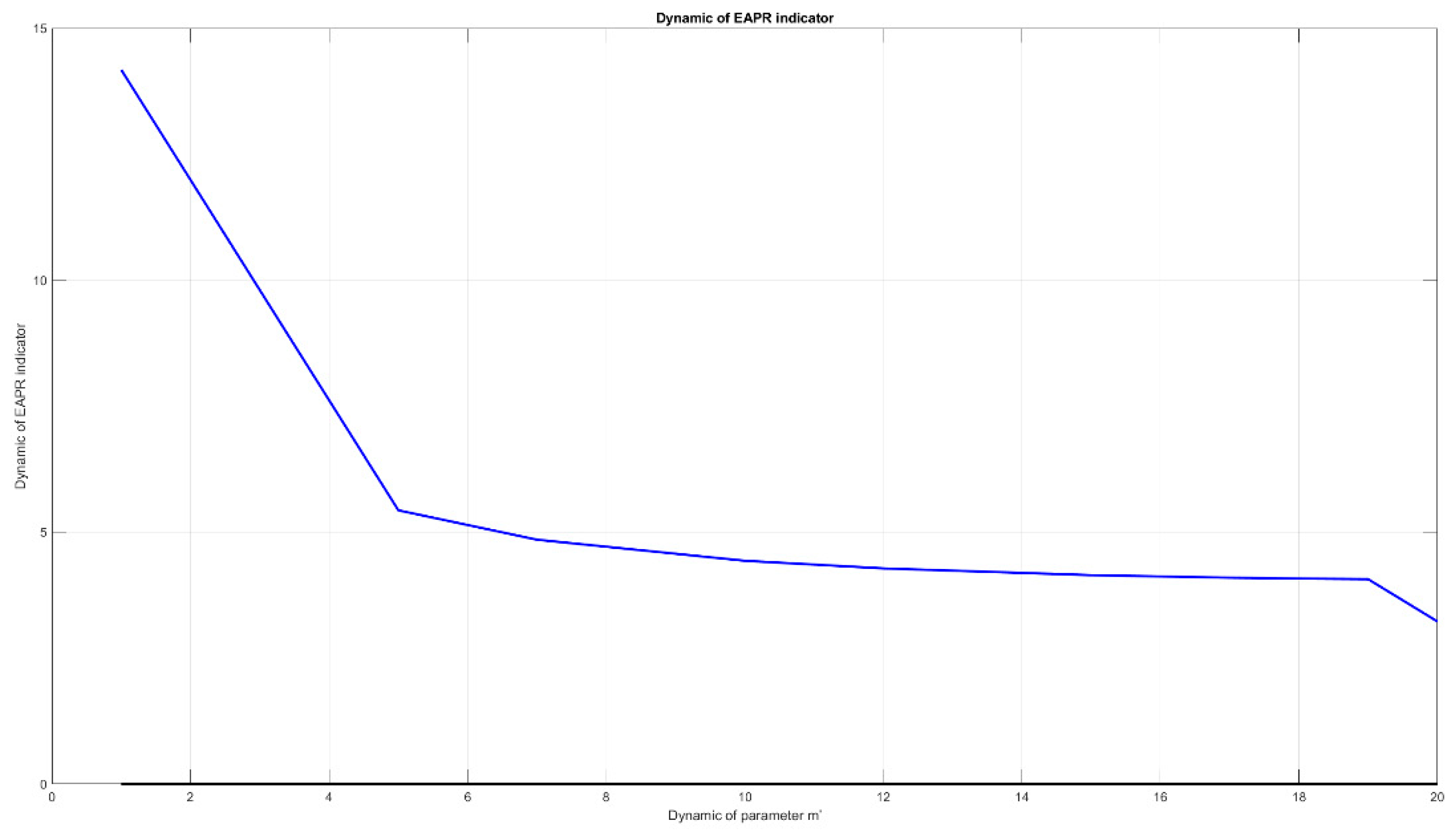
For illustrative purposes of the aforementioned description, the EAPR indicator variation curve is reported below when the “m’” parameter of Equation (48) changes in order to calculate the temporal dynamics of variation of the updated EAPR rate, actualized at the time of contractual stipulation t₀:

In Figure 1 we report an instance of EAPR dynamic curve for a loan structured as follows (

Table 5. Loan amortization parameters.

Principal Amount (Euro Currency)	APR (%)	Periodicity	Day Count Convention	Total Amount of Included “One-Off” Fees (Euro Currency)	Total Amount of Included Recurring Fees (Euro Currency)
250,000.00	3.00	Half-yearly	360/360	2400.00	2.00/installment

):

Unfortunately, even in this case, the contractual information is often not very transparent or is incomplete (therefore asymmetric) as the temporal dynamics of variation of the EAPR rate are almost never indicated and reported according to the possible evolution of amortization but, rather, the only punctual indication of a single value of the EAPR rate, usually the minimum, since the latter obviously is not representative of the real cost of the loan borne by the customer during the repayment plan.

5. Discussion

In this section, as a demonstration of what has been described in the previous paragraphs, we report financial benchmarks deduced from loan contracts typically offered in the retail and corporate market, highlighting the differences in terms of onerousness that derive from the various amortization hypotheses deductible from the contractual clauses. From the analysis of the tables and the benchmark graphs shown below, it will be possible to determine and quantify with extreme precision the additional cost that the borrower is often to pay due to the asymmetric contractual information widely described in this document. We describe two example of loan (one of C = 100,000.00 and another one with C = 250,000.00 both in euro currency) showing—for each of them—the onerousness that derives from the amortization according to the schemes described in the third section of this document. At the end, we highlight such comparison graphs in terms of accrued interests for each amortization schedules.

Specifically, in

Table 6. Loan amortization parameters—example number 1.

Principal Amount (Euro Currency)	APR (%)	Periodicity	Day Count Convention	Total Amount of Included “One-Off” Fees (Euro Currency)	Total Amount of Included Recurring Fees (Euro Currency)
100,000.00	5.00	Monthly (m = 12)	360/360	1500.00	5.00/installment

,

Table 7. Loan amortization schedule Number 1—example number 1.

Principal Amount (Euro Currency)	APR (%)	Periodicity	Day Count Convention	APR/Monthly (%)	EIR (%)
100,000.00	5.00	Monthly (m = 12)	360/360	APR/12	5.11619

,

Table 8. Loan amortization schedule number 1: Onerousness of the loan—example number 1.

Principal Amount (Euro Currency)	APR (%)	Periodicity	Day Count Convention	Total amount of Paid Interests (Euro Currency)	EIR (%)
100,000.00	5.00	Monthly (m = 12)	360/360	27,278.62	5.11619

,

Table 9. Loan amortization schedule number 2—example number 1.

Principal Amount (Euro Currency)	APR (%)	Periodicity	Day Count Convention	APR/monthly (%)	EIR (%)
100,000.00	5.00	Monthly (m = 12)	360/360	$i_{1/m}={\left(1+APR\right)}^{\frac{1}{m}}-1$	5.00

,

Table 10. Loan amortization schedule number 2: Onerousness of the loan—example number 1.

Principal Amount (Euro Currency)	APR (%)	Periodicity	Day Count Convention	Total Amount of Paid Interests (Euro Currency)	EIR (%)
100,000.00	5.00	Monthly (m = 12)	360/360	26,628.24	5.00

,

Table 11. Loan amortization schedule number 3—example number 1.

Principal Amount (Euro Currency)	APR (%)	Periodicity	Day Count Convention	APR/Monthly (%)	EIR (%)
100,000.00	5.00	Monthly (m = 12)	360/360	Simple Interest	5.00

,

Table 12. Loan amortization schedule number 3: Onerousness of the loan—example number 1.

Principal Amount (Euro Currency)	APR (%)	Periodicity	Day Count Convention	Total Amount of Paid Interests (Euro Currency)	EIR (%)
100,000.00	5.00	Monthly (m = 12)	360/360	24,034.62	5,00

,

Table 13. Loan amortization parameters—example number 2.

Principal Amount (Euro Currency)	APR (%)	Periodicity	Day Count Convention	Total Amount of Included “One-Off” Fees (Euro Currency)	Total Amount of Included Recurring Fees (Euro Currency)
250,000.00	3.00	Quarterly (m = 4)	360/365	2400.00	2.00/installment

,

Table 14. Loan amortization schedule number 1—example number 2.

Principal Amount (Euro Currency)	APR (%)	Periodicity	Day Count Convention	APR/Quarterly (%)	EIR (%)
250,000.00	3.00	Quarterly (m = 4)	360/365	APR/4	3.034076

,

Table 15. Loan amortization schedule number 1: Onerousness of the loan—example number 2.

Principal Amount (Euro Currency)	APR (%)	Periodicity	Day Count Convention	Total Amount of Paid Interests (Euro Currency)	EIR (%)
250,000.00	3.00	Quarterly (m = 4)	360/365	39,724.47	3.034076

,

Table 16. Loan amortization schedule number 2—example number 2.

Principal Amount (Euro Currency)	APR (%)	Periodicity	Day Count Convention	APR/Quarterly (%)	EIR (%)
250,000.00	3.00	Quarterly (m = 4)	360/365	$i_{1/m}={\left(1+APR\right)}^{\frac{1}{m}}-1$	3.00

,

Table 17. Loan amortization schedule number 2: Onerousness of the loan—example number 2.

Principal Amount (Euro Currency)	APR (%)	Periodicity	Day Count Convention	Total amount of Paid Interests (Euro Currency)	EIR (%)
250,000.00	3.00	Quarterly	360/365	39,263.45	3.00

,

Table 18. Loan amortization schedule number 3—example number 2.

Principal Amount (Euro Currency)	APR (%)	Periodicity	Day Count Convention	APR/Quarterly (%)	EIR (%)
250,000.00	3.00	Quarterly (m = 4)	360/365	Simple Interest	3.00

and

Table 19. Loan amortization schedule number 3: Onerousness of the loan—example number 2.

Principal Amount (Euro Currency)	APR (%)	Periodicity	Day Count Convention	Total Amount of Paid Interests (Euro Currency)	EIR (%)
250,000.00	3.00	Quarterly (m = 4)	360/365	36,186.37	3.00

the authors reported two examples of a loan amortized according to the algorithmic schemes described in Section 3 of this document and with reference to the same financed principal amount. From the comparison in terms of onerousness of the various amortization plans of the agreed principal as represented in Figure 2, Figure 3, Figure 4 and Figure 5, it is clear that at par of contractual conditions it is possible to amortize the capital in different ways, each having a very specific effective EIR interest rate and an EAPR. The above-described well represents the cost that the borrower has to pay due to the asymmetric contractual information described above, which translates into a broad discretion for the bank regarding the amortization algorithm applicable in practice.

The following Figure 3 shows the cumulative paid interests for each amortization schedule to be applied to the same loan as per Table 6.

As shown in Figure 3, with the same contractual parameters in relation to the agreed loan, the amortization algorithm could be applied in different ways resulting, for each of them, in a very specific effective interest rate, therefore causing higher or lower interest costs for the borrower.

6. Conclusions

The mathematical analysis of the main loan repayment algorithms in relation to the main contractual clauses in the loan contracts normally offered to retail and corporate customers has allowed us to determine the practical consequences that the information asymmetry typically found in the characterization of the repayment plan generates for the customer. The higher costs not highlighted or not easily understood by the contractual indicators, together with a more or less marked discretion in the field of choice of the lending bank, make it clear that this discrepancy between the information agreed upon and made known to the borrower and the actual operative, generates in practice for the borrower hidden (even significant) costs and therefore, a greater burden, which would seem to be one of the main reasons for the increase in default rates of the companies and the insolvency of the loans (the so-called NPLs issue i.e., the nonperforming loans management). Obviously, the absence of transparency or the presence of hidden costs is certainly not the only determining factor in the increase in default or insolvency rates linked to both the retail and corporate customers, as these obviously must also be linked to negative market trends or to problems of another nature that, however, are beyond the theme of this contribution. However, it is clear that the presence of hidden costs in loan contracts can certainly have an impact on the borrowers’ finances and therefore, ultimately, on their ability to repay the contracted debt. The above issues can be addressed in two ways. The first solution the author proposes is related to use of embedded STM32-based device, in which a deep learning natural language programming algorithm is running as firmware (Mazzillo et al. 2018; Ortis et al. 2013; F. Rundo et al. 2018). The results of automatic loan contract language processing allow us to determine the main features of the analyzed contract (principal amount, amortization schedule, APR rate, etc.). After that, an automatic amortization analysis algorithmic engine will be in charge to perform the analysis as described in Section 3. At the end, the system will provide as output the actual costs of the analyzed loan in terms of effective interest rate, EAPR, etc. The following Figure 6 shows the proposed pipeline:

The second solution the author proposes is to extend the typical set of financial information to be included in the loan contract. As shown in Section 3, there is not enough to indicate the APR and such information about the proposed amortization schedule. Rather, it is needed to add information about effective interest rates as well as actual costs that the client will have to face during the repayment of the contracted debt. In other words, the function that maps the space of the contractual parameters to the amortization algorithm actually adopted must be bijective, or rather it must allow the set of agreed financial parameters to correspond to one and only one amortization plan applicable to the interest rate indicated in the contract, zeroing out entirely any discretion in the bank regarding interpretative choices applicable due to unclear, asymmetrical, or ambiguous contractual clauses.

Further works aim to perform a nonlinear pattern analysis (by means of a specific embedded device) of the interest curve, in order to determine such features useful for early diagnosis of the default risk of the borrower (Rundo et al. 2019a; Rundo et al. 2017; Conoci et al. 2017). The author is analyzing the impact of some amortization schemes that have been applied in the healthcare market, rather than others, with particular reference to investments in the oncology field—specifically in relation to the considerably expensive chemotherapy treatments (Banna et al. 2018). The author is also analyzing specific applications of interest rate dynamics to such applications in the field of automatic trading systems (Rundo et al. 2018; Rundo et al. 2019b; Rundo et al. 2019c). Moreover, the authors are studying the correlation between defaults and insolvencies for the customers (in particular for companies) that have requested loan contracts with respect to some contractual parameters of these banking contracts. In doing this, they are obtaining particularly interesting results through the use of a particular correlation function (Ortis et al. 2013). The results of this study will be presented in a forthcoming contribution.

References

1. Banna, Giuseppe L., Andrea Camerini, Giuseppe Bronte, Giuseppe Anile, Alfredo Addeo, Francesco Rundo, Guido Zanghi, Rohit Lal, and Massimo Libra. 2018. Oral metronomic vinorelbine in advanced non-small cell lung cancer patients unfit for chemotherapy. Anticancer Research 38: 3689–97. [Google Scholar] [CrossRef]
2. Brealey, Richard A., Stewart C. Myers, Franklin Allen, and Pitabas Mohanty. 2000. Principles of Corporate Finance, 6th ed. London: Irwin McGraw-Hill, p. 49. [Google Scholar]
3. Conoci, Sabrina, Francesco Rundo, Salvatore Petralta, and Sebastiano Battiato. 2017. Advanced skin lesion discrimination pipeline for early melanoma cancer diagnosis towards PoC devices. Paper presented at IEEE European Conference on Circuit Theory and Design, ECCTD 2017, Catania, Italy, October 31. [Google Scholar]
4. Directive 2014/17/EU. 2014. Directive on credit agreements for consumers relating to residential immovable property and amending Directives 2008/48/EC and 2013/36/EU and Regulation (EU) No 1093/2010. Official Journal of the European Union L 60: 35–85. [Google Scholar]
5. Kellison, Stephen G. 1970. The Theory of Interest. Homewood: Richard D. Irwin, Inc., p. 45. [Google Scholar]
6. Lasher, William. 2008. Practical Financial Management. San Francisco: Thomson South-Western, p. 230. ISBN 0-324-42262-8. [Google Scholar]
7. Mazzillo, Massimo, Lidia Maddiona, Francesco Rundo, Antonella Sciuto, Sebania Libertino, Salvatore Lombardo, and Giorgio Fallica. 2018. Characterization of sipms with nir long-pass interferential and plastic filters. IEEE Photonics Journal 10: 1–12. [Google Scholar] [CrossRef]
8. Ortis, Alessandro, Francesco Rundo, Giuseppe Di Giore, and Sebastiano Battiato. 2013. Adaptive compression of stereoscopic images. In ICIAP 2013, Lecture Notes in Computer Science. Berlin/Heidelberg: Springer, vol. 8156, pp. 391–99. [Google Scholar]
9. Peng, Xing-Ting. 2009. The Real Estate Fictionization: Related to the Theory and Empirical Analysis of United States Subprime Mortgage Crisis. Paper presented at IEEE Second International Conference on Information and Computing Science, Manchester, UK, May 21–22; pp. 147–50. [Google Scholar]
10. Ross, Stephen A., Randolph W. Westerfield, and Bradford D Jordan. 2000. Fundamentals of Corporate Finance. Boston: Irwin/McGraw-Hill, p. 175. ISBN 0-07-231289-0. [Google Scholar]
11. Rundo, Francesco, Sabrina Conoci, Giuseppe L. Banna, Filippo Stanco, and Sebastiano Battiato. 2017. Bio-Inspired Feed-Forward System for Skin Lesion Analysis, Screening and Follow-Up. In International Conference on Image Analysis and Processing. Cham: Springer, vol. 10485, pp. 399–409. [Google Scholar]
12. Rundo, Francesco, Sabrina Conoci, Giuseppe L. Banna, Alessandro Ortis, Filippo Stanco, and Sebastiano Battiato. 2018. Evaluation of Levenberg–Marquardt neural networks and stacked autoencoders clustering for skin lesion analysis, screening and follow-up. IET Computer Vision 12: 957–62. [Google Scholar] [CrossRef]
13. Rundo, Francesco, Salvatore Petralia, Giorgio Fallica, and Sabrina Conoci. 2019a. A nonlinear pattern recognition pipeline for PPG/ECG medical assessments. Lecture Notes in Electrical Engineering 539: 473–80. [Google Scholar]
14. Rundo, Francesco, Francesca Trenta, Agatino Di Stallo, and Sebastiano Battiato. 2019b. Advanced Markov-Based Machine Learning Framework for Making Adaptive Trading System. Computation 7: 4. [Google Scholar] [CrossRef]
15. Rundo, Francesco, Francesca Trenta, Agatino Luigi di Stallo, and Sebastiano Battiato. 2019c. Grid Trading System Robot (GTSbot): A Novel Mathematical Algorithm for Trading FX Market. Applied Sciences 9: 1796. [Google Scholar] [CrossRef]
16. Tang, Junjun, Jing Wang, Cheng Huang, Guolun Wang, and Xiong Wang. 2008. Subprime Mortgage Crisis Detection in U.S. Foreign Exchange Rate Market by Multifractal Analysis. Paper presented at IEEE 9th International Conference for Young Computer Scientists, Zhang Jia Jie, China, November 18–21; pp. 2999–3004. [Google Scholar]
17. Tian, Hou-Ping, and Chang-Xian Liu. 2007. Contract Design in Mortgage Loans under Asymmetric Information: The Analysis When Firms are Short of Mortgage Assets. Paper presented at IEEE International Conference on Wireless Communications, Networking and Mobile Computing, Honolulu, HI, USA, August 12–16; pp. 4626–29. [Google Scholar]
18. Zhu, Zheng-Xuan, and Zu Yan. 2013. Prediction model of mortgage prepayment risk. Paper presented at IEEE International Conference on Management Science & Engineering, Philadelphia, PA, USA, November 7–9; pp. 418–23. [Google Scholar]
Figure 1. Dynamic of the the effective annual percentage interest rate (EAPR) indicator with the variation of the parameter m’ of the Equation (48).
Economies 07 00091 g001
Figure 2. Amortization schedule of the loan reported in Table 6: (a) Cumulative interests; (b) amount of principal for each payment; (c) amount of interests for each payment; (d) decreasing outstanding balance.
Economies 07 00091 g002
Figure 3. Benchmark in terms of paid interests for the loan reported in Table 6: The blue curve represents the cumulative paid interests for amortization schedule number 1 (Table 8); the red curve represents the cumulative paid interests for amortization schedule number 2—APR = EAPR—(Table 10); the black curve represents the cumulative paid interests for amortization schedule number 3—simple interest—(Table 12).
Economies 07 00091 g003
Figure 4. Amortization schedule of the loan reported in Table 13: (a) Cumulative interests; (b) amount of principal for each payment; (c) amount of interests for each payment; (d) decreasing outstanding balance.
Economies 07 00091 g004
Figure 5. Benchmark in terms of paid interests for the loan reported in Table 14: The blue curve represents the cumulative paid interests for amortization schedule number 1 (Table 15); the red curve represents the cumulative paid interests for amortization schedule number 2—APR = EAPR—(Table 17); the black curve represents the cumulative paid interests for amortization schedule number 3—simple interest—(Table 19).
Economies 07 00091 g005
Figure 6. The proposed deep learning STM32-based pipeline for automatic loan contract analysis.
Economies 07 00091 g006