Article

Gas Sensing with Nanoporous In2O3 under Cyclic Optical Activation: Machine Learning-Aided Classification of H2 and H2O

Department of Chemistry, Paderborn University, Warburger Str. 100, D-33098 Paderborn, Germany
*
Author to whom correspondence should be addressed.
Chemosensors 2024, 12(9), 178; https://doi.org/10.3390/chemosensors12090178
Submission received: 9 July 2024 / Revised: 7 August 2024 / Accepted: 29 August 2024 / Published: 3 September 2024

Abstract

:
Clean hydrogen is a key aspect of carbon neutrality, necessitating robust methods for monitoring hydrogen concentration in critical infrastructures like pipelines or power plants. While semiconducting metal oxides such as In2O3 can monitor gas concentrations down to the ppm range, they often exhibit cross-sensitivity to other gases like H2O. In this study, we investigated whether cyclic optical illumination of a gas-sensitive In2O3 layer creates identifiable changes in a gas sensor’s electronic resistance that can be linked to H2 and H2O concentrations via machine learning. We exposed nanostructured In2O3 with a large surface area of 95 m2 g−1 to H2 concentrations (0–800 ppm) and relative humidity (0–70%) under cyclic activation utilizing blue light. The sensors were tested for 20 classes of gas combinations. A support vector machine achieved classification rates up to 92.0%, with reliable reproducibility (88.2 ± 2.7%) across five individual sensors using 10-fold cross-validation. Our findings suggest that cyclic optical activation can be used as a tool to classify H2 and H2O concentrations.

Graphical Abstract

1. Introduction

Over the past decade, a growing emphasis on sustainable energy solutions has led to a surge in research and development in the field of hydrogen-based technologies. As part of this trend, the European Union’s hydrogen strategy for a climate-neutral Europe has highlighted the increasing need for reliable and efficient hydrogen detection technologies [1]. At the core of these technologies are semiconducting metal oxides, which have the remarkable property of changing their electrical resistance upon exposure to reactive gas species. A detailed description of the resistance changes of semiconductors (in particular In2O3) upon gas exposure is described in the literature [2,3]. Metal oxides with a large surface area are attractive for gas sensing applications, such as mesoporous Indium(III) oxide (In2O3), due to the large number of surface adsorption sites that amplify the resistance change compared to non-porous materials. When the metal oxide is synthesized by a structure replication process on the nanometer scale (i.e., nanocasting), it possesses a well-defined structure enabling specific, target-oriented applications [4]. In nanocasting, ordered mesoporous silica is used as a mold, infiltrated with an indium oxide precursor (indium nitrate in this case), that is thermally converted to the oxide. After selective removal of the silica mold, nanostructured In2O3 remains [5].
Indium(III) oxide is a well-known n-type semiconductor with a surprisingly high charge carrier concentration of up to 1010 cm−3 [6]. Its large electrical conductivity is attributed to oxygen deficiency in the lattice and many intrinsic defects under a reducing atmosphere [7]. Therefore, In2O3 is a great candidate for low-temperature gas measurements. Illumination with sub-bandgap energy (e.g., blue LED, 472 nm, 2.6 eV) can be utilized because of the above-mentioned defects (In2O3 bandgap values reported in the literature range from 2.1 eV to 3.7 eV [8,9,10]) to increase sensor response and kinetics. Upon illumination, desorption of oxygen adsorbates and photo-reduction are two of several reasons why the electronic resistance of In2O3 changes [6,11,12,13]. These effects can also be used in photocatalytic applications [14,15].
Despite these advantages, resistive gas sensors might suffer from a lack of selectivity, meaning their inability to differentiate between different gases simultaneously [16,17]. To increase selectivity, various approaches can be pursued, such as adding barrier (filter) layers [18], catalysts [19,20,21], variation of measurement voltage [22], or temperature cycling [23,24,25,26,27] to create multi-signals [28,29,30,31]. Temperature cycling can be conducted in sub-second cycles when using appropriate sensor systems [32]. It should be noted that the sensor’s chemical response may be the rate-determining step [23,33,34] when using optical activation. Optical activation might not affect the whole sensing layer because the penetration depth of, e.g., UV light in dense In2O3 is around 10 nm [35,36]. This fact emphasizes the need for nanostructured metal oxides for optical activation in gas sensing because the radiation can penetrate deeper into the material due to the porosity. Materials synthesized by nanocasting are particularly interesting because their wall thickness is in the range of small mesopores (2–15 nm) and, therefore, in the same dimensions as the penetration depth of (UV-)light. Also, particle size and the sensing layer thickness need to be considered [37]. Constant optical activation, i.e., permanent illumination of a gas sensor by a light source, is already well-investigated and summarized in review articles [2,12,38]. However, transient optical activation is a novel trend in the resistive gas sensor community [39,40,41,42].
The forced change in sensor conductivity by variable illumination helps overcome the conductivity drifts that are often observed in resistive gas sensors due to the equilibration of the sensor, which can take from minutes to days [13,43]. If a gas sensor is exposed to discrete gas concentrations, and these are used for learning and prediction, a classification algorithm is a common tool of choice. Therefore, a support vector machine (SVM; e.g., a classifier) was utilized in this study to classify the gas concentration by means of resistance value changes upon illumination [44]. Ten-fold cross-validation was utilized for learning and classification. The application of machine learning techniques is becoming more and more popular to overcome challenges in physical chemistry and gas sensor measurements in particular [13,45,46,47].
Recently, Schmuker et al. investigated the limitations of machine learning in gas sensing due to baseline drift [48,49]. They discussed baseline changes in the data that are limiting the usability of machine learning for concentration classification. For this reason, Ge et al. extracted the gas-specific features from the data and used them for gas identification. In this way, the aging effects of the sensor as well as changes in the environmental conditions could be suppressed in the training data [50]. Siadat et al. describe the utilization of sample set partitioning (SPXY) to select their training data and an SVM regression for monitoring air pollution [51]. Their calibration method proved to be quite efficient and reliable compared to classical direct standardization. SVM methods seem to address the quantification and differentiation between different gas species quite well. As shown by Yang et al., zinc oxide in different morphologies can create an array of gas sensors differentiating methanol, ethanol, propanol, acetone, formaldehyde, and ammonia [52]. A linear ridge classifier underperformed compared to the SVM classifier, which was correct in 99% of gas classifications. Furthermore, concentration classification for ethanol showed a strong performance of 98%.
Yoon and Park introduced transient illumination with UV light when using an In2O3 sensor decorated with gold nanoparticles to classify gas types (acetone, NO2, ethanol, methanol, and air) and concentration (0–100 ppm). The pseudo-random change in illumination intensity led to electronic resistance changes that could be analyzed by a deep neural network. Gas-type classification resulted in an accuracy of 96% for a single gas sensor [13].
This study explores whether cyclic optical activation can be used to classify discrete H2 and H2O concentrations via an SVM. High surface area In2O3 without dopants is used as a gas-sensitive layer and is exposed to varied hydrogen gas (0–800 ppm) and water (0–70%) concentrations in synthetic air. Five individual sensors were utilized to test for classification reproducibility. Both H2 and H2O lower the electronic resistance of nanostructured In2O3, posing differentiation challenges that might occur in stationary power or an automotive context [53].

2. Materials and Methods

Synthesis of mesoporous silica: Ordered mesoporous silica number 6 from Korean Institute of Technology (KIT-6) [54] was synthesized by dissolving block co-polymer Pluronic P-123 (8.0 g, Sigma Aldrich, St. Louis, MO, USA, Mn~5800) in deionized water (240 mL), hydrochloric acid (28.6 g mL, 35%, Stockmeier, Bielefeld, Germany), and butan-1-ol (8.0 g, Stockmeier, Bielefeld, Germany) at 35 °C. After the addition of tetraethyl orthosilicate (16 g, 98%, Sigma-Aldrich, St. Louis, MO, USA), the solution is stirred for 24 h (35 °C), followed by hydrothermal treatment at 80 °C for 24 h in a glass-lined autoclave. After filtration and washing (three times) with water, the white precipitate is dried at 60 °C for 24 h. Finally, the polymer is thermally decomposed in a furnace at 550 °C for 5 h (2.5 °C min−1).
Synthesis of mesoporous In2O3: Ordered mesoporous In2O3 was structurally replicated from cubic KIT-6 silica according to the procedure outlined in the literature [55]. A mortar, pistil, and silica were warmed to 100 °C in a drying cabinet. The amount of indium nitrate pentahydrate (99.99%, Sigma-Aldrich, St. Louis, MO, USA) was calculated by multiplying the silica mass with the pore volume of silica and the density of the molten precursor (around 2.4 mL g−1), aiming to fill the pores completely. The indium nitrate was added to the preheated mortar as well as the preheated silica. Both components were homogenized and treated at 85 °C for 24 h. The composite was heated in an open vessel in a furnace under air to a temperature of 300 °C with a heating rate of 2 °C min−1 for 2 h to convert the indium nitrate to the indium oxide.
The silica matrix is removed by leaching with a NaOH solution (5 mol L−1, Stockmeier, Bielefeld, Germany) at a temperature of 60 °C for one hour. After centrifugation (4000 rpm for 15 min), the liquid phase is removed. This procedure was repeated three times. The remaining solid was washed with deionized water until a pH value of 7 was reached. The indium oxide was dried at a temperature of 60 °C for 24 h prior to further usage.
Material characterization: N2 physisorption measurements were conducted at −196 °C after degassing the samples at 120 °C for 12 h in a vacuum using an Autosorb 6 (Quantachrome Instruments, Boca Raton, FL, USA). Surface areas were calculated using the Brunauer–Emmet–Teller (BET [56]) approach in a relative pressure region of 0.1–0.3, meeting the Rouquerol requirements [57]. Pore size distributions were calculated from the desorption branch, utilizing the Barrett–Joyner–Halenda model [58] as well as non-local density functional theory (NLDFT) kernel for cylindrical silica pores. The total pore volume was calculated at the penultimate adsorption point.
Diffraction data were collected on a AXS D8 advance (Bruker, Karlsruhe, Germany) with Cu Kα radiation (40 kV, 40 mA) with a step size of 2θ of 0.0075° (below 5°) and a step time of 300 s, and a step size of 0.02° (above 5°) with a step time of 3 s, respectively.
Particle size of In2O3 was determined by averaging over 25 particles collected on a Neon 40 scanning electron microscope (SEM, Zeiss, Oberkochen, Germany).
A Ultra Dry detector (Thermo Fisher Scientific, Waltham, MA, USA) determined residual silica content and In:O ratio from energy-dispersive X-ray spectroscopy.
The UV-vis spectrum was measured on a Lambda 650 (PerkinElmer, Waltham, MA, USA).
Gas sensor preparation and measurement: Mesoporous indium oxide (25 mg) was dispersed in deionized water (1 mL) and treated for 5 min in an ultrasonic bath. Then, 2 µL of the dispersion was dropped onto interdigitated electrodes (UST, sensor substrate 3 × 3 mm with IDS, 10 Ohm platinum heating element, mounted on T039 base, Geratal, Germany) and the sensor was dried at room temperature. Five individual sensors were prepared. Prior to the measurements, the sensors were first treated at 350 °C for 24 h and then at the measurement temperature of 150 °C for an additional 28 d. Resistance measurements (measured with 10 Hz) were performed under a constant gas flow of 500 mL min−1 with different concentrations of hydrogen (0–800 ppm; Air Liquid) and relative humidity (0–70%) in synthetic air (20.5% O2, 79.5% N2, Air Liquid). Humidity values refer to carrier gas at a temperature of 22 °C. The sensor substrates were illuminated using a blue LED (InGaN, clear, 4.9 mm diameter, 8.6 mm height, peak wavelength 472 nm, FWHM = 40 nm, Luckylight, LL-504BC2E-B4-2GC) utilizing a square-wave voltage of 2.72 V. The distance of the LED to the gas sensor substrate was 10.7 mm with a radiation angle of 15°, leading to a light power of around 49 mW cm−2. A so-called cycle contains an illumination period (5 s), followed by 5 s without illumination, and therefore lasts 10 s in total.
Machine learning analysis: The machine learning analysis serves the purpose of analyzing resistance changes of the gas sensor upon illumination that then can be correlated to experimental conditions, i.e., discrete gas concentrations. The experimental data (i.e., electronic resistance and gas concentrations) were used without any data clean-up or preprocessing for the discussion in Section 3.3. Subsets of the data were used as described in Section 3.4. and Section 3.5. Additionally, the normalization of data cycles was investigated as discussed in Section 3.4. Data analysis was performed using the Scikit-learn package [59]. A support vector machine with a linear kernel was used (regularization parameter C = 0.01). An unequal sample size was dealt with by undersampling. Ten-fold cross-validation was used for training and learning.

3. Results and Discussion

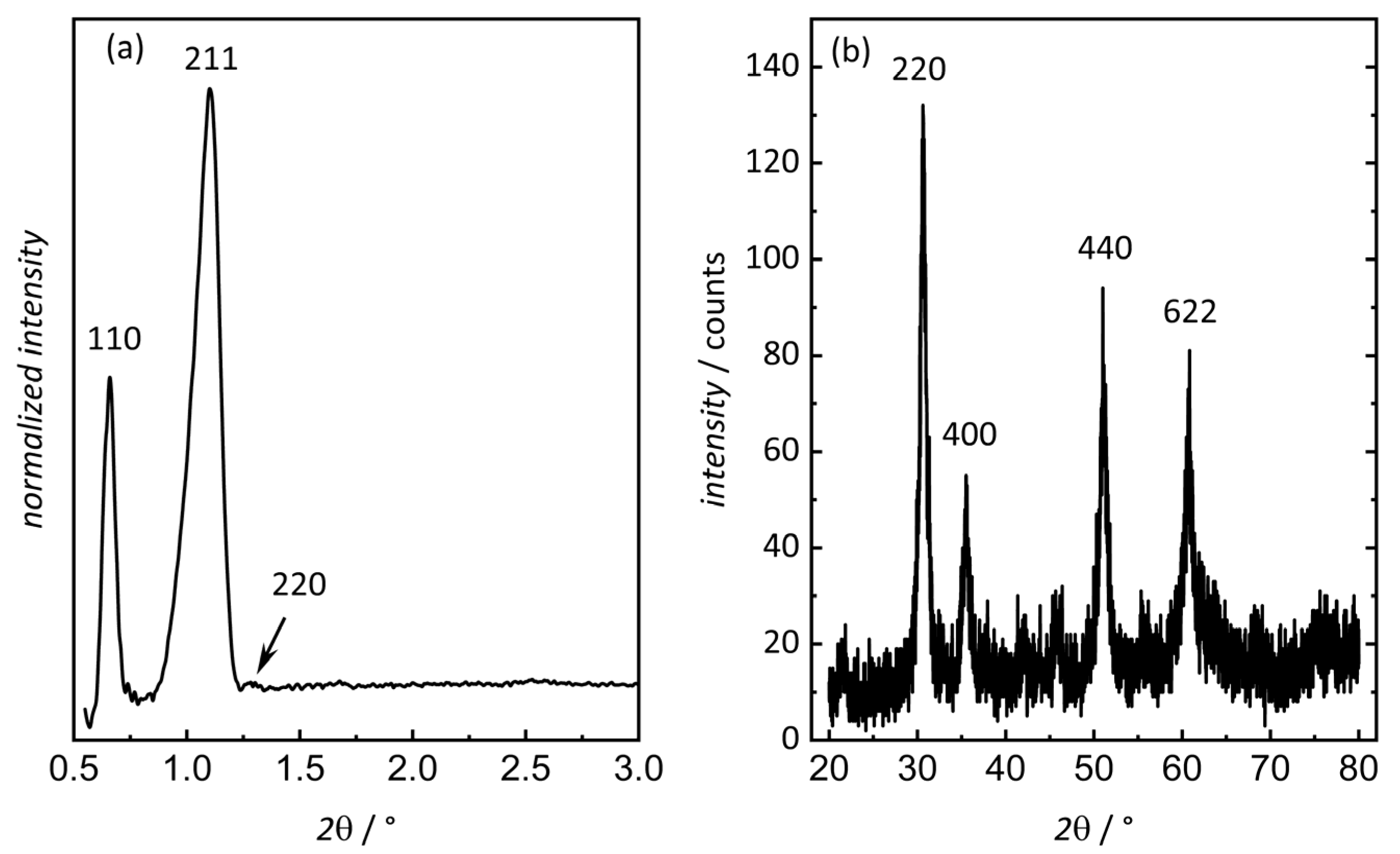
3.1. Characterization of Ordered Mesoporous In2O3

In2O3 is nanocasted from mesoporous silica (for characterization see Figures S1 and S2; physisorption raw data are available in .aif format [60] in the Electronic Supplementary Information Section) and characterized by N2 physisorption, as depicted in Figure 1. The metal oxide exhibits a surface area of 95 m2 g−1 and a total pore volume of 0.62 cm3 g−1 (see Table 1). These values are larger compared to bulk metal oxides, especially when considering the apparent density of In2O3.
A type IV isotherm with two steps in a relative pressure region between 0.6 and 0.92 and small hysteresis can be observed. The isotherm and hysteresis shape indicate a successful nanocasting procedure and a mesoporous material with two maxima in the pore size distribution (Figure 1b). The smaller pore mode (6.0 nm BJH, 8.1 nm NLDFT) originates from the replication of the silica matrix. The larger mesopore (12.3 nm BJH, 14.5 nm NLDFT) is attributed to a partial displacement of the two interpenetrating pore networks, as described in the literature [55,61].
The displacement results in a lower symmetry of the metal oxide ( I 4 1 / a or lower) compared to the silica ( I a 3 ¯ d ), which is supported by the appearance of 110 in the low-angle diffractogram (Figure 2a), which is symmetry forbidden in I a 3 ¯ d [61]. Reflections at larger angles are not visible anymore, which is due to the reduced degree of pore ordering or can be attributed to accidental extinction depending on the diameter of the metal oxide rods. The wide-angle diffraction pattern in Figure 2b confirms a successful synthesis of polycrystalline (cubic bixbyite structure, I a 3 ¯ ) In2O3. The crystallite size of around 11 nm was determined via the Scherrer method, based on the 220 reflection. This fits well with the determined pore size, which restricts the unimpaired crystal growth of In2O3, thereby limiting the crystallite size [62].
The In2O3 particles exhibit a spherical shape with an average particle size of around 95 ± 5 nm (Figure 3), and the cubic pore structure is clearly visible. The atomic ratio of In to O is 0.59 ± 0.08: 1 which, with respect to the error of the measurement, resembles In2O3. The remaining silica content is around 3.4 ± 0.94 wt.%, which might be one reason for the atomic ratio of In to O showing a slight excess of oxygen. The synthesized In2O3 exhibits a direct bandgap of 3.83 ± 0.002 eV (see Figure S3).

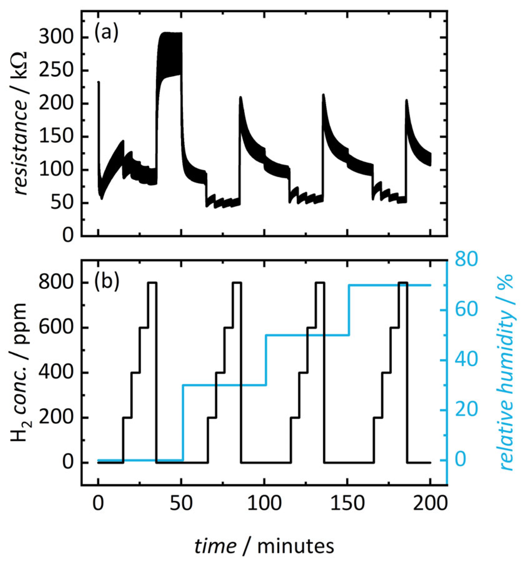
3.2. Resistance Changes during Cyclic Optical Activation and Gas Exposure

Cyclic optical activation was performed by illuminating a gas-sensitive In2O3 layer with light from a blue LED for five seconds, leading to a decrease in electronic resistance that bounces back after the LED is switched off for five seconds, which is repeated throughout the entire measurement and therefore referred to as cyclic optical activation.
A representative part of the resistance over time measurement at a constant atmosphere is shown in Figure 4. Illumination of the metal oxide layer on top of the interdigital electrode leads to oxygen desorption, photoreduction, and therefore a drop in resistance [6,11,12]. The electronic resistance depends on the atmosphere during the measurement and lies in a range between 100 kΩ and 340 kΩ for this particular gas sensor.
The sensor exhibits an electric resistance of around 230 kΩ at the start of the measurement that drops down to about 80 kΩ at the beginning of the first illumination cycle (as shown in Figure 5). The sensor’s resistance increases afterward because the dry synthetic air removes adsorbed water from the surface of the metal oxide.
Resistive gas sensors can take from minutes to days to achieve a stable baseline [43]. Fifteen minutes after starting the measurement, hydrogen (200 ppm) is added even though the baseline is still changing (i.e., the sensor is operated under non-equilibrium conditions for a fast concentration readout). A total of five sensors were prepared, four of which are shown in the Supplementary Information Section (Figure S4).
Adding a reducing gas leads to a decrease in electric resistance in an n-type semiconductor. Here, the hydrogen concentration was increased every 5 min in steps of 200 ppm until 800 ppm was reached. Afterward, the hydrogen addition was stopped, increasing resistance up to around 310 kΩ. Increasing the relative humidity to 30% reduces the resistance due to the adsorption of water on the sensor’s surface [63]. This general trend can be observed for all humidity levels. The sensor was exposed to five different concentrations of hydrogen (0 ppm, 200 ppm, 400 ppm, 600 ppm, and 800 ppm) and four relative humidity values (0%, 30%, 50%, and 70%), leading to a total of 20 different classes of gas concentrations.
Classical approaches to interpreting a gas sensor’s resistance typically wait for a stable baseline and a stable signal after a change of atmosphere. The change in resistance R (or response, which is resistance divided by base resistance R0) is then associated with specific gas concentrations. As mentioned above, these processes can take a long time, especially at low temperatures. Therefore, we refrain from long waiting times and utilize machine learning to classify the resistance data, even though the sensors are far from reaching equilibrium.

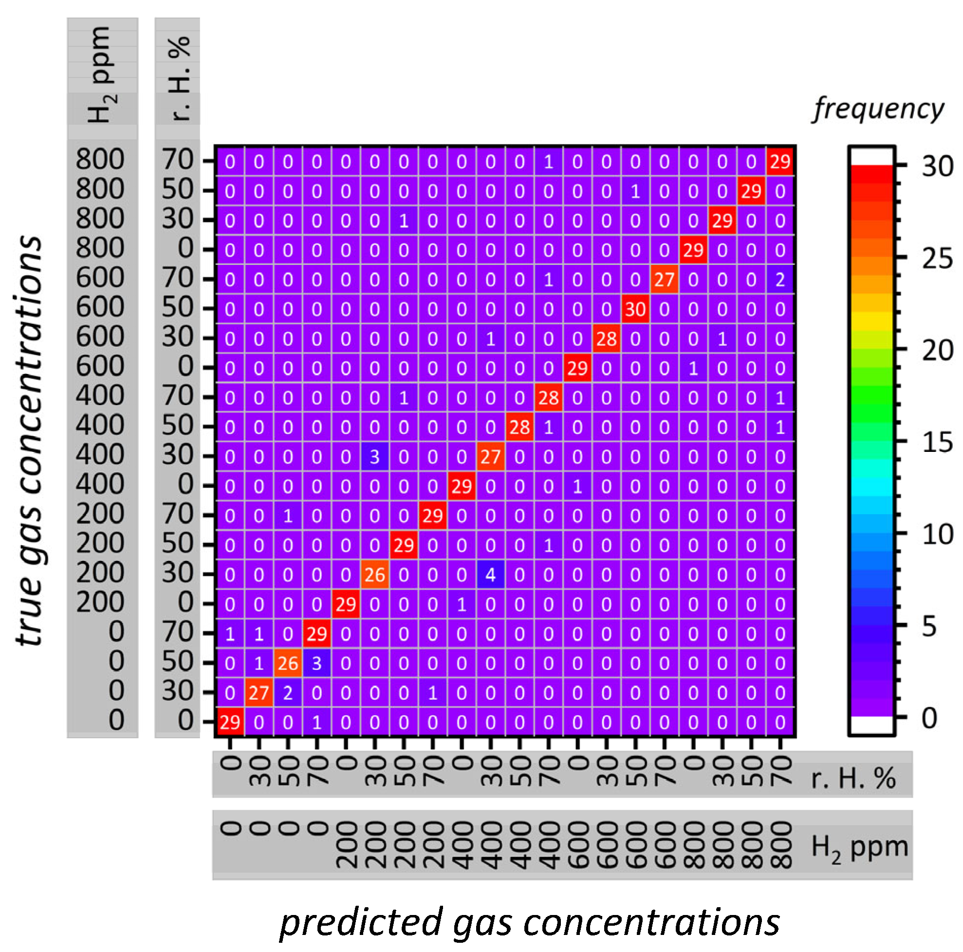
3.3. Gas Concentration Classification

The gas sensor was exposed to discrete amounts of hydrogen (five concentrations: 0 ppm, 200 ppm, 400 ppm, 600 ppm, and 800 ppm) and relative humidity (four concentrations: 0%, 30%, 50%, and 70%) and the changes in the electronic resistance upon gas and light exposure (full cycle for a total of 10 s with a resistance measurement frequency of 10 Hz) were used for learning and evaluation of the classes. No gas concentrations between the aforementioned classes were added or evaluated, so we chose a classification algorithm. The actual concentrations (i.e., classes) versus the classification made by the machine learning algorithm are depicted in a confusion matrix in Figure 6. Cycles located on the diagonal (from bottom left to top right) are correctly classified sets, while deviations from the diagonal are wrongly associated. The best sensor (out of five) exhibits a correct classification of 92.0%, which is comparable to the literature values (see Table 2).
Four more sensors were prepared, measured, and evaluated in the same way to estimate the method’s reliability. It turns out that the accuracy of the gas concentration classification and discrimination between hydrogen and humidity was 88.2 ± 2.7% over five individual sensors, which is a little below the literature data (see Table 2). However, not many studies compare several sensors in parallel as we did in this study. Static and dynamic temperatures can lead to higher classification rates than our data; however, one must consider the semiconductors and gases investigated. The results presented by Yoon and Park et al. are the closest to our study (utilizing In2O3 decorated with Au particles), where a single sensor was investigated, leading to a classification rate of 96.53% using transient illumination and deep-learning [13].
Prior to the detailed analysis of the data using SVM, we conducted a brief screening utilizing other methods to see which approach potentially leads to the best classification rates. We investigated decision tree (62.0 ± 11.6%), k-nearest neighbor (67.8 ± 10.0%), multilayer perceptron (50 hidden layers, 21.0 ± 5.7%), and Gaussian process model analysis (39.0 ± 11.1%) for the presented five individual gas sensors. Furthermore, we conducted a principal component analysis. A full illumination–darkness cycle was split into half, and then both parts separately fitted against a power function to reduce dimensionality (from 100 to 4; e.g., analysis of slope and curvature for both half cycles) followed by classification. The classification rate was 50.75 ± 7.5%. When performed effectively, target-oriented dimensionality reduction can lead to enhanced sensor performance, which can be an interesting direction for future data evaluation [64]. A regression-based assessment is shown in the Supplementary Information section (Figure S5) for comparison. Due to the classification rate success of utilizing SVM, we decided to evaluate the data further.
Table 2. Classification rate based on literature results compared to this study.
Faleh
et al.
[65]
Tonezzer,
Van Duy
et al.
[27]
Kim,
Shin
et al.
[66]
Ge
et al.
[50]
Yoon,
Park
et al.
[13]
This
Study
materialWO3SnO2 + Ag, PtZnOcommercialIn2O3 + AuIn2O3
no. sensor(s)441115
operation modestatic
T a
static
T a
cyclic
T a
cyclic
T a
time-variant
illumination
cyclic
illumination
data analysisSVMSVMCNN bSVMCNN bSVM
data preprocessingyesnoyesyesyesno
classification rate/%93.0310093.995.496.5392.0
a T = temperature, b CNN = convolutional neural networks.

3.4. Single-Gas Concentration Classification and Cycle Normalization

In the analysis so far, both offered gases were taken into account when it comes to the classification of concentrations. The group-based approach described in this subsection assesses the model’s robustness by testing its ability to generalize to new data combinations. When only using constant H2 concentrations, e.g., 0 ppm and training with 0–75% r. H. (the second column in Table 3 shows the classification rate from data collected during t = 0–15 min, 35–65 min, 85–115 min, 135–165 min, and 185–200 min), the classification rate of H2O was around 79.8 ± 8.5%, which is comparably low compared to the other classes (see Table 3). This effect might be related to a substantial drift in electronic resistance as the setup, including heating and gasflow, was switched on at t = 0 min, which is usually uncommon for resistive gas measurements. It is quite widespread that resistive gas sensors are kept at constant conditions (temperature and atmosphere) for periods ranging from minutes up to several hours to avoid influencing data interpretation. This might be the reason why the classification rate is higher for constant H2 concentrations of 200–800 ppm, as sensor drift might affect these regions less because the sensor had a longer operation period.
When only constant H2O concentrations (e.g., 0% r. H. which is shown in column two in Table 4) were taken into account, classification levels were between around 95–98%, as summarized in Table 3.
Furthermore, a model was used where the training data consisted of relative humidity values except for 50%, which was then tested for. The classification rate was about 72.3 ± 4.0%. When doing the same for H2 concentrations (learning with 0 ppm, 200 ppm, 600 ppm, and 800 ppm of H2) and testing for 400 ppm, the algorithm was correct in 41.5 ± 10.3%. We tested how cycle normalization between 0 and 1 affected the results to elucidate the importance of absolute electric resistance on the classification rate. The classification rate after normalization (of each individual cycle) drops to 31.6 ± 5.7% over all five sensors. These results lead to the assumption that the absolute resistance plays a significant role in the classification process. This might also explain why it is not possible with our approach to learn with four individual sensors and classify the gas concentrations of the fifth sensor (see also ESI Figure S4.) and why PCA was less reliable when testing on the data set. The results indicate that overfitting by the algorithm is an issue that surfaces via the cross-validation. In this approach, the training data always contain similar gas concentration values compared to the data that is to be classified. Therefore, the algorithm struggles to interpret unknown data, which can be seen in the group-based approach.

3.5. Classification Success for Different Stages of the Optical Activation Process

We tried to test whether parts of the illumination (or darkness) cycle lead to similar classification rates. Therefore, the data were divided into subsets to identify the importance of certain parts of the measurement for the classification algorithm. Figure 7 shows four different kinds of (sub)datasets.
As already discussed, if the entire measurement is utilized (LED on and off for 5 s each, 10 s total) the gas concentration classification accuracy is 88.4% (Figure 7a). The accuracy reduces to 80.4 ± 4.5% if the data were utilized from when the LED is on for 5 s (b) and 81.2 ± 6.0% when the LED is off for 5 s (c), respectively. If the data for classification are chosen from the middle part of the darkness–illumination cycle (2.5 darkness, 2.5 s illumination) as depicted in (d), accuracy is about 86.6 ± 4.5%, as summarized in Table 5.
The evaluation of the subset of data shows that a data reduction, i.e., using 5 s of a cycle, slightly decreases when the data is split into half (10 s total illumination–darkness cycle for (a) and only 5 s for every case form (b)–(d)). Therefore, it seems that the necessary information for the classification can be found in every subset investigated above, which again points towards the influence of absolute resistance on the classification rate. However, overfitting needs to be taken into account, as discussed previously.

4. Conclusions

This study successfully demonstrates a unique approach of integrating machine learning with resistive gas sensing, utilizing cyclic optical illumination to classify H2 (0 ppm–800 ppm) and H2O (0–70%) concentrations. Using a gas-sensitive In2O3 layer, cyclically illuminated with sub-bandgap energy, enabled us to employ a linear support vector machine for classification. This method achieved a classification rate of up to 92.0% using 10-fold cross-validation, maintaining high accuracy across five individual sensors (88.2 ± 2.7%).
However, we observed a decrease in accuracy when splitting learning data into half, and a strong decrease when normalizing individual cycles. While these aspects present limitations in our current model, they offer valuable insights for further investigations. Notably, our findings underline the substantial potential of combining cyclic optical activation and machine learning for gas sensing. A careful balance between the complexity of the model and the available data is required.
Increasing the amount of training data and reducing dimensionality could enhance classification rates in future studies. Furthermore, we would vary the illumination frequency, light intensity, and activation wavelength to investigate the classification rate and feature extraction, and potentially differentiate between other gases and gas concentrations at a time, especially with the rising interest in the global H2 market. This aspect could be particularly interesting for industrial applications such as fuel cell monitoring or catalytic conversion of CO (e.g., PROX process). Moreover, unraveling the underlying mechanism of identifying and associating features to gas concentrations could improve the sensor system. The integration of artificial intelligence with traditional sensing technologies, as shown in our study, indicates a promising and exciting pathway for future research in the field of gas sensing.

Supplementary Materials

The following supporting information can be downloaded at: https://www.mdpi.com/article/10.3390/chemosensors12090178/s1. Figure S1: N2 physisorption isotherm and pore size distribution (of mesoporous KIT-6 silica; N2 physisorption raw data for mesoporous silica and mesoporous In2O3 are attached as well; Figure S2: Low-angle X-ray diffraction pattern of mesoporous KIT-6 silica with double gyroidal structure; Figure S3: Transmission spectrum and Tauc plot of mesoporous In2O3; Figure S4: resistance changes over time for four resistive gas sensors; Figure S5: k-nearest neighbor regression. The raw data of the gas sensor measurements are available as well.

Author Contributions

D.B.: methodology, software, validation, formal analysis, investigation, data curation, writing—review and editing, visualization; A.K.: methodology, software, validation, formal analysis, investigation, data curation, writing—review and editing; M.T.: conceptualization, resources; T.W.: conceptualization, resources, funding acquisition; C.W.: conceptualization, methodology, writing—original draft, visualization, supervision, project administration. All authors have read and agreed to the published version of the manuscript.

Funding

This research was funded by the German Federal Ministry of Education and Research (BMBF, 13XP5024B). We highly appreciate the support.

Institutional Review Board Statement

Not applicable.

Informed Consent Statement

Not applicable.

Data Availability Statement

The data that support the findings of this study are available from the corresponding author upon reasonable request.

Acknowledgments

The authors thank Gerald Njio for setting up the measurement hardware.

Conflicts of Interest

The authors declare no conflicts of interest.

References

  1. European Commission. Communication from the Commision to the European Parliament, the Council, the European Economics and Social Committee and the Committee of the Regions: A Hydrogen Strategy for Climate-Neutral Europe. Available online: https://ec.europa.eu/energy/sites/ener/files/hydrogen_strategy.pdf (accessed on 3 July 2024).
  2. Xu, F.; HO, H.-P. Light-Activated Metal Oxide Gas Sensors: A Review. Micromachines 2017, 8, 333. [Google Scholar] [CrossRef]
  3. Li, Z.; Yan, S.; Wu, Z.; Li, H.; Wang, J.; Shen, W.; Wang, Z.; Fu, Y. Hydrogen gas sensor based on mesoporous In2O3 with fast response/recovery and ppb level detection limit. Int. J. Hydrogen Energy 2018, 43, 22746–22755. [Google Scholar] [CrossRef]
  4. Wagner, T.; Haffer, S.; Weinberger, C.; Klaus, D.; Tiemann, M. Mesoporous materials as gas sensors. Chem. Soc. Rev. 2013, 42, 4036–4053. [Google Scholar] [CrossRef] [PubMed]
  5. Gu, D.; Schüth, F. Synthesis of non-siliceous mesoporous oxides. Chem. Soc. Rev. 2014, 43, 313–344. [Google Scholar] [CrossRef] [PubMed]
  6. Kohl, C.-D.; Wagner, T.; Dickert, F.L.; Dickert, F.L. (Eds.) Gas Sensing Fundamentals; Springer: Berlin/Heidelberg, Germany, 2014; ISBN 978-3-642-54518-4. [Google Scholar]
  7. Shah, S.; Hussain, S.; Din, S.T.U.; Shahid, A.; Amu-Darko, J.N.O.; Wang, M.; Tianyan, Y.; Liu, G.; Qiao, G. A review on In2O3 nanostructures for gas sensing applications. J. Environ. Chem. Eng. 2024, 12, 112538. [Google Scholar] [CrossRef]
  8. Xirouchaki, C.; Kiriakidis, G.; Pedersen, T.F.; Fritzsche, H. Photoreduction and oxidation of as-deposited microcrystalline indium oxide. J. Appl. Phys. 1996, 79, 9349–9352. [Google Scholar] [CrossRef]
  9. Matino, F.; Persano, L.; Arima, V.; Pisignano, D.; Blyth, R.I.R.; Cingolani, R.; Rinaldi, R. Electronic structure of indium-tin-oxide films fabricated by reactive electron-beam deposition. Phys. Rev. B 2005, 72, 85437. [Google Scholar] [CrossRef]
  10. Spencer, J.A.; Mock, A.L.; Jacobs, A.G.; Schubert, M.; Zhang, Y.; Tadjer, M.J. A review of band structure and material properties of transparent conducting and semiconducting oxides: Ga2O3, Al2O3, In2O3, ZnO, SnO2, CdO, NiO, CuO, and Sc2O3. Appl. Phys. Rev. 2022, 9, 011315. [Google Scholar] [CrossRef]
  11. Wagner, T.; Kohl, C.D.; Morandi, S.; Malagù, C.; Donato, N.; Latino, M.; Neri, G.; Tiemann, M. Photoreduction of Mesoporous In2O3: Mechanistic Model and Utility in Gas Sensing. Chem. Eur. J. 2012, 18, 8216–8223. [Google Scholar] [CrossRef]
  12. Espid, E.; Taghipour, F. UV-LED Photo-activated Chemical Gas Sensors: A Review. Crit. Rev. Solid State Mater. Sci. 2017, 42, 416–432. [Google Scholar] [CrossRef]
  13. Cho, I.; Lee, K.; Sim, Y.C.; Jeong, J.-S.; Cho, M.; Jung, H.; Kang, M.; Cho, Y.-H.; Ha, S.C.; Yoon, K.-J.; et al. Deep-learning-based gas identification by time-variant illumination of a single micro-LED-embedded gas sensor. Light Sci. Appl. 2023, 12, 95. [Google Scholar] [CrossRef] [PubMed]
  14. Lu, Y.; Shao, L.; Deng, S.; Lu, Z.; Yan, R.; Ren, D.; Huang, Y.; Liu, H. Synthesis of C-In2O3/BiOI composite and its enhanced photocatalytic degradation for methyl blue. Inorg. Chem. Commun. 2019, 100, 56–59. [Google Scholar] [CrossRef]
  15. Wang, Y.; Zhang, J.; Balogun, M.-S.; Tong, Y.; Huang, Y. Oxygen vacancy–based metal oxides photoanodes in photoelectrochemical water splitting. Mater. Today Sustain. 2022, 18, 100118. [Google Scholar] [CrossRef]
  16. Eranna, G.; Joshi, B.C.; Runthala, D.P.; Gupta, R.P. Oxide Materials for Development of Integrated Gas Sensors—A Comprehensive Review. Crit. Rev. Solid State Mater. Sci. 2004, 29, 111–188. [Google Scholar] [CrossRef]
  17. Schultealbert, C.; Amann, J.; Baur, T.; Schütze, A. Measuring Hydrogen in Indoor Air with a Selective Metal Oxide Semiconductor Sensor. Atmosphere 2021, 12, 366. [Google Scholar] [CrossRef]
  18. van den Broek, J.; Weber, I.C.; Güntner, A.T.; Pratsinis, S.E. Highly selective gas sensing enabled by filters. Mater. Horiz. 2021, 8, 661–684. [Google Scholar] [CrossRef]
  19. Dey, A. Semiconductor metal oxide gas sensors: A review. Mater. Sci. Eng. B 2018, 229, 206–217. [Google Scholar] [CrossRef]
  20. Ueda, T.; Boehme, I.; Hyodo, T.; Shimizu, Y.; Weimar, U.; Barsan, N. Enhanced NO2-Sensing Properties of Au-Loaded Porous In2O3 Gas Sensors at Low Operating Temperatures. Chemosensors 2020, 8, 72. [Google Scholar] [CrossRef]
  21. Weber, I.C.; Güntner, A.T. Catalytic filters for metal oxide gas sensors. Sens. Actuators B 2022, 356, 131346. [Google Scholar] [CrossRef]
  22. Sauerwald, T.; Skiera, D.; Kohl, C.-D. Selectivity enhancement of gas sensors using non-equilibrium polarisation effects in metal oxide films. Appl. Phys. A 2007, 87, 525–529. [Google Scholar] [CrossRef]
  23. Gramm, A.; Schütze, A. High performance solvent vapor identification with a two sensor array using temperature cycling and pattern classification. Sens. Actuators B 2003, 95, 58–65. [Google Scholar] [CrossRef]
  24. Lee, A. Temperature modulation in semiconductor gas sensing. Sens. Actuators B 1999, 60, 35–42. [Google Scholar] [CrossRef]
  25. Semancik, S.; Cavicchi, R.E.; Wheeler, M.C.; Tiffany, J.E.; Poirier, G.E.; Walton, R.M.; Suehle, J.S.; Panchapakesan, B.; DeVoe, D.L. Microhotplate platforms for chemical sensor research. Sens. Actuators B 2001, 77, 579–591. [Google Scholar] [CrossRef]
  26. Leidinger, M.; Sauerwald, T.; Reimringer, W.; Ventura, G.; Schütze, A. Selective detection of hazardous VOCs for indoor air quality applications using a virtual gas sensor array. J. Sens. Sens. Syst. 2014, 3, 253–263. [Google Scholar] [CrossRef]
  27. Thai, N.X.; Tonezzer, M.; Masera, L.; Nguyen, H.; van Duy, N.; Hoa, N.D. Multi gas sensors using one nanomaterial, temperature gradient, and machine learning algorithms for discrimination of gases and their concentration. Anal. Chim. Acta 2020, 1124, 85–93. [Google Scholar] [CrossRef]
  28. Smulko, J.; Trawka, M.; Ionescu, R.; Annanouch, F.E.; ETSE-DEEEA, E.L.; Granqvist, C.G.; Kish, L.B. New approaches for improving selectivity and sensitivity of resistive gas sensors: A review. Int. J. Smart Sens. Intell. Syst. 2014, 7, 1–6. [Google Scholar] [CrossRef]
  29. Güney, S.; Atasoy, A. Multiclass classification of n-butanol concentrations with k-nearest neighbor algorithm and support vector machine in an electronic nose. Sens. Actuators B 2012, 166–167, 721–725. [Google Scholar] [CrossRef]
  30. Reimann, P.; Schütze, A. Sensor Arrays, Virtual Multisensors, Data Fusion, and Gas Sensor Data Evaluation. In Gas Sensing Fundamentals; Kohl, C.-D., Wagner, T., Dickert, F.L., Dickert, F.L., Eds.; Springer: Berlin/Heidelberg, Germany, 2014; pp. 67–107. ISBN 978-3-642-54518-4. [Google Scholar]
  31. Dorst, T.; Schneider, T.; Eichstädt, S.; Schütze, A. Influence of measurement uncertainty on machine learning results demonstrated for a smart gas sensor. J. Sens. Sens. Syst. 2023, 12, 45–60. [Google Scholar] [CrossRef]
  32. Ankara, Z.; Kammerer, T.; Gramm, A.; Schütze, A. Low power virtual sensor array based on a micromachined gas sensor for fast discrimination between H2, CO and relative humidity. Sens. Actuators B 2004, 100, 240–245. [Google Scholar] [CrossRef]
  33. Prades, J.D.; Jimenez-Diaz, R.; Hernandez-Ramirez, F.; Barth, S.; Cirera, A.; Romano-Rodriguez, A.; Mathur, S.; Morante, J.R. Equivalence between thermal and room temperature UV light-modulated responses of gas sensors based on individual SnO2 nanowires. Sens. Actuators B 2009, 140, 337–341. [Google Scholar] [CrossRef]
  34. Njio, G.; Wagner, T. P2AR.3—Virtual Gas Sensor Array by Cyclic Optical Activation: Optimization of Activation Profile by Machine Learning. In Proceedings of the 17th International Meeting on Chemical Sensors—IMCS 2018, Vienna, Austria, 15–19 July 2018; AMA Service GmbH: Wunstorf, Germany, 2018; pp. 905–906. [Google Scholar]
  35. Agoston, P.; Albe, K. Formation entropies of intrinsic point defects in cubic In2O3 from first-principles density functional theory calculations. Phys. Chem. Chem. Phys. 2009, 11, 3226–3232. [Google Scholar] [CrossRef] [PubMed]
  36. Bender, M.; Katsarakis, N.; Gagaoudakis, E.; Hourdakis, E.; Douloufakis, E.; Cimalla, V.; Kiriakidis, G. Dependence of the photoreduction and oxidation behavior of indium oxide films on substrate temperature and film thickness. J. Appl. Phys. 2001, 90, 5382–5387. [Google Scholar] [CrossRef]
  37. Klaus, D.; Klawinski, D.; Amrehn, S.; Tiemann, M.; Wagner, T. Light-activated resistive ozone sensing at room temperature utilizing nanoporous In2O3 particles: Influence of particle size. Sens. Actuators B 2015, 217, 181–185. [Google Scholar] [CrossRef]
  38. Chizhov, A.; Rumyantseva, M.; Gaskov, A. Light Activation of Nanocrystalline Metal Oxides for Gas Sensing: Principles, Achievements, Challenges. Nanomaterials 2021, 11, 892. [Google Scholar] [CrossRef] [PubMed]
  39. Nasriddinov, A.; Tokarev, S.; Fedorova, O.; Bozhev, I.; Rumyantseva, M. In2O3 Based Hybrid Materials: Interplay between Microstructure, Photoelectrical and Light Activated NO2 Sensor Properties. Chemosensors 2022, 10, 135. [Google Scholar] [CrossRef]
  40. Nasriddinov, A.; Rumyantseva, M.; Konstantinova, E.; Marikutsa, A.; Tokarev, S.; Yaltseva, P.; Fedorova, O.; Gaskov, A. Effect of Humidity on Light-Activated NO and NO2 Gas Sensing by Hybrid Materials. Nanomaterials 2020, 10, 915. [Google Scholar] [CrossRef] [PubMed]
  41. Rumyantseva, M.; Nasriddinov, A.; Krivetskiy, V.; Gaskov, A. Light—Assisted Low Temperature Formaldehyde Detection at Sub-ppm Level Using Metal Oxide Semiconductor Gas Sensors. Proceedings 2019, 14, 37. [Google Scholar] [CrossRef]
  42. Rumyantseva, M.; Nasriddinov, A.; Vladimirova, S.; Tokarev, S.; Fedorova, O.; Krylov, I.; Drozdov, K.; Baranchikov, A.; Gaskov, A. Photosensitive Organic-Inorganic Hybrid Materials for Room Temperature Gas Sensor Applications. Nanomaterials 2018, 8, 671. [Google Scholar] [CrossRef]
  43. Lee, D.-Y.; Yu, J.-B.; Byun, H.-G.; Kim, H.-J. Chemoresistive Sensor Readout Circuit Design for Detecting Gases with Slow Response Time Characteristics. Sensors 2022, 22, 1102. [Google Scholar] [CrossRef]
  44. Dulhare, U.; Ahmad, K.; Bin Ahmad, K. Machine Learning and Big Data, 1st ed.; Wiley-Scrivener; Safari: Boston, MA, USA, 2020; ISBN 9781119654742. [Google Scholar]
  45. Yaqoob, U.; Younis, M.I. Chemical Gas Sensors: Recent Developments, Challenges, and the Potential of Machine Learning—A Review. Sensors 2021, 21, 2877. [Google Scholar] [CrossRef]
  46. Ferguson, A.L.; Hachmann, J.; Miller, T.F.; Pfaendtner, J. The Journal of Physical Chemistry A / B / C Virtual Special Issue on Machine Learning in Physical Chemistry. J. Phys. Chem. C 2020, 124, 24033–24038. [Google Scholar] [CrossRef]
  47. Prezhdo, O.V. Advancing Physical Chemistry with Machine Learning. J. Phys. Chem. Lett. 2020, 11, 9656–9658. [Google Scholar] [CrossRef] [PubMed]
  48. Dennler, N.; Rastogi, S.; Fonollosa, J.; van Schaik, A.; Schmuker, M. Drift in a popular metal oxide sensor dataset reveals limitations for gas classification benchmarks. Sens. Actuators B 2022, 361, 131668. [Google Scholar] [CrossRef]
  49. Vergara, A.; Fonollosa, J.; Mahiques, J.; Trincavelli, M.; Rulkov, N.; Huerta, R. On the performance of gas sensor arrays in open sampling systems using Inhibitory Support Vector Machines. Sens. Actuators B 2013, 185, 462–477. [Google Scholar] [CrossRef]
  50. Ge, H.; Liu, J. Identification of gas mixtures by a distributed support vector machine network and wavelet decomposition from temperature modulated semiconductor gas sensor. Sens. Actuators B Chem. 2006, 117, 408–414. [Google Scholar] [CrossRef]
  51. Laref, R.; Losson, E.; Sava, A.; Siadat, M. Support Vector Machine Regression for Calibration Transfer between Electronic Noses Dedicated to Air Pollution Monitoring. Sensors 2018, 18, 3716. [Google Scholar] [CrossRef]
  52. Wang, T.; Ma, H.; Jiang, W.; Zhang, H.; Zeng, M.; Yang, J.; Wang, X.; Liu, K.; Huang, R.; Yang, Z. Type discrimination and concentration prediction towards ethanol using a machine learning-enhanced gas sensor array with different morphology-tuning characteristics. Phys. Chem. Chem. Phys. 2021, 23, 23933–23944. [Google Scholar] [CrossRef] [PubMed]
  53. Boon-Brett, L.; Bousek, J.; Black, G.; Moretto, P.; Castello, P.; Hübert, T.; Banach, U. Identifying performance gaps in hydrogen safety sensor technology for automotive and stationary applications. Int. J. Hydrogen Energy 2010, 35, 373–384. [Google Scholar] [CrossRef]
  54. Kleitz, F.; Hei Choi, S.; Ryoo, R. Cubic Ia3d large mesoporous silica: Synthesis and replication to platinum nanowires, carbon nanorods and carbon nanotubes. Chem. Commun. 2003, 17, 2136–2137. [Google Scholar] [CrossRef]
  55. Klaus, D.; Amrehn, S.; Tiemann, M.; Wagner, T. One-step synthesis of multi-modal pore systems in mesoporous In2O3: A detailed study. Microporous Mesoporous Mater. 2014, 188, 133–139. [Google Scholar] [CrossRef]
  56. Brunauer, S.; Emmett, P.H.; Teller, E. Adsorption of Gases in Multimolecular Layers. J. Am. Chem. Soc. 1938, 60, 309–319. [Google Scholar] [CrossRef]
  57. Rouquerol, J.; Llewellyn, P.; Rouquerol, F. Is the BET equation applicable to microporous adsorbents? In Studies in Surface Science and Catalysis Characterization of Porous Solids VII, Proceedings of the 7th International Symposium on the Characterization of Porous Solids (COPS-VII), Aix-en-Provence, France, 26–28 May 2005; Llewellyn, P.L., Ed.; Elsevier: Amsterdam, The Netherlands, 2007; pp. 49–56. ISBN 0167-2991. [Google Scholar]
  58. Barrett, E.P.; Joyner, L.G.; Halenda, P.P. The Determination of Pore Volume and Area Distributions in Porous Substances. I. Computations from Nitrogen Isotherms. J. Am. Chem. Soc. 1951, 73, 373–380. [Google Scholar] [CrossRef]
  59. Pedregosa, F.; Varoquaux, G.; Gramfort, A.; Michel, V.; Thirion, B.; Grisel, O.; Blondel, M.; Prettenhofer, P.; Weiss, R.; Dubourg, V.; et al. Scikit-learn: Machine Learning in Python. J. Mach. Learn. Res. 2011, 12, 2825–2830. [Google Scholar]
  60. Evans, J.D.; Bon, V.; Senkovska, I.; Kaskel, S. A Universal Standard Archive File for Adsorption Data. Langmuir 2021, 37, 4222–4226. [Google Scholar] [CrossRef] [PubMed]
  61. Kim, T.W.; Solovyov, L.A. Synthesis and characterization of large-pore ordered mesoporous carbons using gyroidal silica template. J. Mater. Chem. 2006, 16, 1445–1455. [Google Scholar] [CrossRef]
  62. Haffer, S.; Waitz, T.; Tiemann, M. Mesoporous In2O3 with Regular Morphology by Nanocasting: A Simple Relation between Defined Particle Shape and Growth Mechanism. J. Phys. Chem. C 2010, 114, 2075–2081. [Google Scholar] [CrossRef]
  63. Suematsu, K.; Ma, N.; Watanabe, K.; Yuasa, M.; Kida, T.; Shimanoe, K. Effect of Humid Aging on the Oxygen Adsorption in SnO2 Gas Sensors. Sensors 2018, 18, 254. [Google Scholar] [CrossRef]
  64. Jia, W.; Sun, M.; Lian, J.; Hou, S. Feature dimensionality reduction: A review. Complex Intell. Syst. 2022, 8, 2663–2693. [Google Scholar] [CrossRef]
  65. Faleh, R.; Gomri, S.; Aguir, K.; Kachouri, A. A new combined transient extraction method coupled with WO3 gas sensors for polluting gases classification. Sens. Rev. 2021, 41, 437–448. [Google Scholar] [CrossRef]
  66. Kim, T.; Kim, Y.; Cho, W.; Kwak, J.-H.; Cho, J.; Pyeon, Y.; Kim, J.J.; Shin, H. Ultralow-Power Single-Sensor-Based E-Nose System Powered by Duty Cycling and Deep Learning for Real-Time Gas Identification. ACS Sens. 2024, 9, 3557–3572. [Google Scholar] [CrossRef]
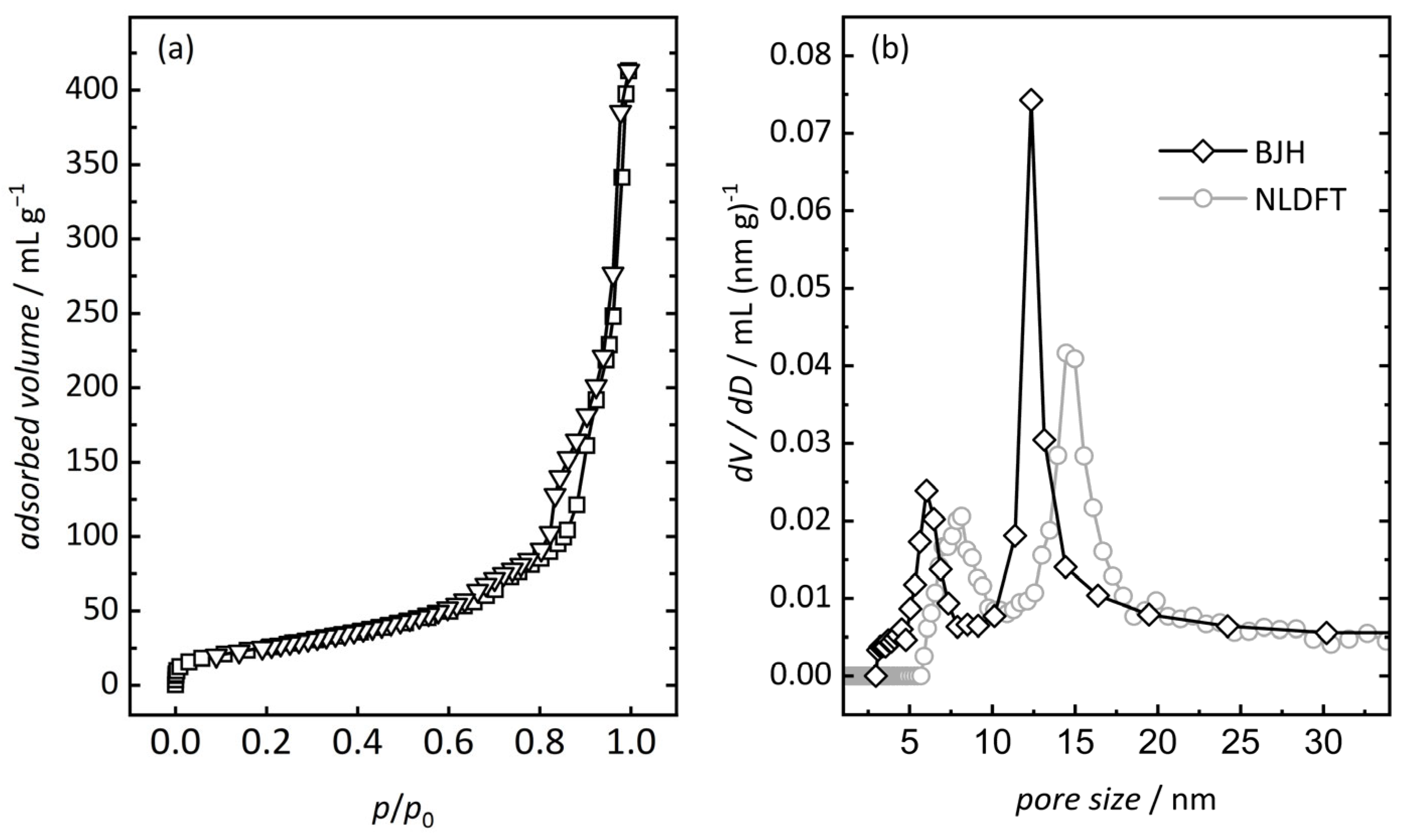
Figure 1. (a) N2 physisorption isotherm) and (b) pore size distribution (BJH black diamonds, NLDFT gray circles) of mesoporous In2O3.
Chemosensors 12 00178 g001
Figure 2. (a) Low-angle and (b) wide-angle powder X-ray diffraction patterns of mesoporous In2O3.
Chemosensors 12 00178 g002
Figure 3. A representative SEM image of mesoporous In2O3, after removing the silica matrix, indicates the cubic symmetry of the pore system.
Chemosensors 12 00178 g003
Figure 4. Representative part of the electric resistance changes over time of mesoporous In2O3 at 150 °C in dependence of LED status (white area LED on, gray area LED off), constant concentration of H2 (0 ppm), and r. H. (50%).
Chemosensors 12 00178 g004
Figure 5. (a) Resistance of mesoporous In2O3 measured at 150 °C upon exposure (b) to hydrogen (0 ppm, 200 ppm, 400 ppm, 600 ppm, and 800 ppm) and relative humidity (0%, 30%, 50%, and 70%). Duration of illumination is 5 s, followed by no illumination for 5 s. Illumination cycling is repeated throughout the entire measurement.
Chemosensors 12 00178 g005
Figure 6. Confusion matrix of the In2O3 gas sensor measurements shown in Figure 5 comparing the predicted classes to the actual classes of hydrogen concentration (0 ppm, 200 ppm, 400 ppm, 600 ppm, and 800 ppm) and relative humidity (0%, 30%, 50%, and 70%).
Chemosensors 12 00178 g006
Figure 7. Data chosen from Figure 5 utilized for classification (white area LED on, gray area LED off, and hatched area shows data utilized for machine learning), (a) full cycle, (b) illumination cycle, (c) darkness cycle, (d) 2.5 s of darkness followed by 2.5 s of illumination. Illumination and darkness periods are set to 5 s each.
Chemosensors 12 00178 g007
Table 1. N2 physisorption derived values of the silica matrix and the nanostructured In2O3.
SamplePore Size (a)
nm
Pore Size (b)
nm
Surface Area (c)
m2 g−1
Pore Volume (d)
mL g−1
silica5.16.65500.83
In2O36.0; 12.38.1; 14.5950.62
(a) derived from BJH model (desorption branch); (b) derived from NLDFT model (desorption branch), (c) BET surface area; (d) total pore volume.
Table 3. Classification rate of H2O at constant concentrations of H2.
constant H2
concentration [ppm]
0200400600800
H2O classification79.8 ± 8.596.6 ± 1.796.2 ± 1.599.0 ± 1.399.4 ± 0.8
Table 4. Classification rate of H2 at constant concentrations of H2O.
constant H2O
concentration [%]
0305070
H2 classification97.8 ± 1.796.4 ± 0.897.0 ± 1.795.1 ± 1.0
Table 5. Classification rate depending on the utilized dataset.
DatasetLED StatusDuration of
... s
Classification Rate
%
IlluminationDarknessDataset
(a)on-off551088.4 ± 3.0
(b)on50580.4 ± 4.5
(c)off05581.2 ± 6.0
(d)off-on2.52.5586.6 ± 4.5
Disclaimer/Publisher’s Note: The statements, opinions and data contained in all publications are solely those of the individual author(s) and contributor(s) and not of MDPI and/or the editor(s). MDPI and/or the editor(s) disclaim responsibility for any injury to people or property resulting from any ideas, methods, instructions or products referred to in the content.

