Article

The Kansas City Transportation and Local-Scale Air Quality Study (KC-TRAQS): Integration of Low-Cost Sensors and Reference Grade Monitoring in a Complex Metropolitan Area. Part 1: Overview of the Project

1
U.S. Environmental Protection Agency, Office of Research and Development, National Risk Management Research Laboratory, 109 TW Alexander Dr., Research Triangle Park, NC 27711, USA
2
U.S. Environmental Protection Agency, Region 7, 300 Minnesota Ave., Kansas City, KS 66101, USA
3
U.S. Environmental Protection Agency, Office of Research and Development, National Exposure Research Laboratory, 109 TW Alexander Dr., Research Triangle Park, NC 27711, USA
4
U.S. Environmental Protection Agency, Region 7, 11201 Renner Blvd., Lenexa, KS 66219, USA
5
Jacobs Technology Inc., 109 TW Alexander Dr., Research Triangle Park, NC 27711, USA
6
ORISE Participant, U.S. Environmental Protection Agency, Office of Research and Development, National Risk Management Research Laboratory, 109 TW Alexander Dr., Research Triangle Park, NC 27711, USA
7
Science Systems and Applications, Inc., 109 TW Alexander Dr., Research Triangle Park, NC 27711, USA
*
Author to whom correspondence should be addressed.
Chemosensors 2019, 7(2), 26; https://doi.org/10.3390/chemosensors7020026
Submission received: 5 April 2019 / Revised: 15 May 2019 / Accepted: 21 May 2019 / Published: 27 May 2019
(This article belongs to the Special Issue Chemical Sensors for Air Quality Monitoring)

Abstract

:
Emissions from transportation sources can impact local air quality and contribute to adverse health effects. The Kansas City Transportation and Local-Scale Air Quality Study (KC-TRAQS), conducted over a 1-year period, researched emissions source characterization in the Argentine, Turner, and Armourdale, Kansas (KS) neighborhoods and the broader southeast Kansas City, KS area. This area is characterized as a near-source environment with impacts from large railyard operations, major roadways, and commercial and industrial facilities. The spatial and meteorological effects of particulate matter less than 2.5 µm (PM2.5), and black carbon (BC) pollutants on potential population exposures were evaluated at multiple sites using a combination of regulatory grade methods and instrumentation, low-cost sensors, citizen science, and mobile monitoring. The initial analysis of a subset of these data showed that mean reference grade PM2.5 concentrations (gravimetric) across all sites ranged from 7.92 to 9.34 µg/m3. Mean PM2.5 concentrations from low-cost sensors ranged from 3.30 to 5.94 µg/m3 (raw, uncorrected data). Pollution wind rose plots suggest that the sites are impacted by higher PM2.5 and BC concentrations when the winds originate near known source locations. Initial data analysis indicated that the observed PM2.5 and BC concentrations are driven by multiple air pollutant sources and meteorological effects. The KC-TRAQS overview and preliminary data analysis presented will provide a framework for forthcoming papers that will further characterize emission source attributions and estimate near-source exposures. This information will ultimately inform and clarify the extent and impact of air pollutants in the Kansas City area.

Graphical Abstract

1. Introduction

1.1. Environmental and Health Impacts from Transportation Sources

Exposures to ambient concentrations of particulate matter (PM), including PM with an aerodynamic diameter of 2.5 µm or less (PM2.5), have been linked to adverse human health effects, including cardiovascular, respiratory, and premature mortality occurrences [1,2]. For populations engaging in normal day-to-day activities (e.g., living, working, going to school) in close proximity to major freeways/highways, comparable adverse health effects have been reported [1,2,3,4,5]. While these associations have been reported, identification of the specific near-road pollutants of concern has not yet been identified, nor have individual pollutants been linked with particular health outcomes in the near-road environment [3,4,5,6]. Furthermore, far less evidence on air quality around other non-roadway transportation sources has been published. Consequently, understanding the unique micro-air pollutant environment near major transportation facilities is of interest. This includes understanding the contribution of these facilities to the spatial and temporal variability of this micro-environment, as well as PM concentrations and key species, such as black carbon (BC) [4,7]. Numerous studies have shown elevated levels of air pollutants adjacent to major transportation facilities [8,9,10,11,12,13,14,15,16,17]. Reported health effects from these environments include exacerbation of asthma, as well as cardiovascular and non-asthma respiratory symptoms [4]. As urbanization throughout the world continues, more and more of the world’s population will be spending time near large transportation facilities. Currently, it is estimated that 16% of the U.S. population lives within 100 m (300 ft) of a four-or-more lane highway [18,19,20]. The public health implications of millions of people being exposed to transportation-related air pollutants may be considerable.
Multi-modal transportation facilities, defined as the movement of goods between transportation modes (i.e., rail, water, pipeline, truck, air), emit air pollutant species including carbon monoxide (CO), oxides of nitrogen (NO, NO2, NOX), PM with an aerodynamic diameter ≤ 10 µm (PM10), PM2.5, BC, carbon dioxide (CO2), and multiple air toxins. This air pollution may impact communities near these facilities as well as along freight movement corridors. Railyards are just one type of multi-modal transportation facility and are in and of themselves complex emission sources. The emission sources within railyards can vary widely by type and location, including linehaul engines, switching locomotives, and maintenance activities. In addition, railyards usually have other emission sources adjacent or in close proximity (e.g., truck distribution centers, power plants, industry, marine ports), and these other sources can complicate a source characterization study. Additional confounding factors include topography, meteorology, and surrounding buildings [21]. As freight transport continues to expand, rail use will likely increase [22].
Several recent studies have reported on air quality impacts from railyards and multi-modal transportation facilities. The Cicero Railyard Study [23] concluded that during downwind conditions (winds blowing from railyard–from south), air pollutant levels, such as BC, were twice as high than during upwind conditions (winds from the north). This resulted in higher observed BC concentrations in residential areas closest to the railyard. Higher levels of BC were observed during the mobile measurement campaign’s early morning and evening hour driving routes. The observed BC levels were 30%–104% over the urban background levels, which suggests that the increase was associated with railyard activity or morning temperature inversions, which are generally higher in the early morning and evening hours [21,23]. However, under certain operating conditions, such as low-load diesel engines (e.g., idling locomotives, creeping trains), low BC/PM ratios were observed. The Atlanta Railyard Study (mobile measurements and stationary site) [24,25] indicated that there were statistically significant increases in air pollutants, including ultrafine particulates (UFPs) and BC from rail-yard activities, as compared to adjacent background levels. The Roseville Railyard Study [26] concluded that the earlier findings of the California Air Resources Board (CARB) model results of railyard emission impacts were accurate and that the communities downwind of the railyard were at-risk for deleterious health outcomes [26]. Lastly, a study conducted in the multi-modal port environs of Charleston, South Carolina [27] found that neighborhoods adjacent to the port experienced elevated air pollution due to port activities, including goods movement into and out of the port by ship, rail, or truck. Measurements collected downwind and upwind of a Charleston railyard showed median PM2.5 concentrations 19% higher at the downwind site [27].

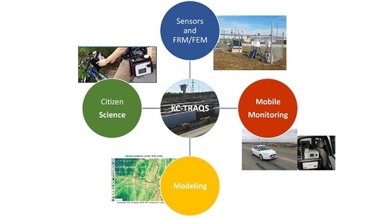
1.2. Kansas City Transportation and Local-Scale Air Quality Study (KC-TRAQS)

The Kansas City Transportation and Local-Scale Air Quality Study (KC-TRAQS), was a field measurement campaign designed to more fully understand community air pollution on a micro-scale, in an area affected by multiple sources. The primary pollutants of interest were PM2.5 and BC. The study aims to answer these questions:
  • What is the spatial and temporal variability of air pollution in the Argentine, Turner, and Armourdale neighborhoods and the broader southeast Kansas City, Kansas (KS) area?
  • Can the impact of local air pollution sources on the Argentine, Turner, and Armourdale neighborhoods and Kansas City area be identified and quantified?
  • What is the air pollution impact from trucking fleets and truck traffic, railyards, and passing railroad traffic under different meteorological conditions and source activities?
  • Can different monitoring technologies and techniques help enhance future transportation air quality research?
This study has multiple unique characteristics including a 1-year duration, site-specific meteorological data, measurement of multiple air pollutant species, and integration of regulatory grade methods and instrumentation, low-cost sensors, citizen science, and mobile monitoring. This paper describes the KC-TRAQS study design and presents an initial analysis of PM2.5 and BC data collected from select reference grade instruments and low-cost sensors. This paper is not intended to address all of the study aims listed above. More focused papers on these topics are forthcoming.

2. Study Design

The KC-TRAQS design included three measurement platforms: (1) stationary site instruments with a focus on PM2.5 and BC measurements, (2) citizen science data collection using low-cost sensor devices, and (3) mobile monitoring. The specific methods and instruments used for these measurement platforms are described in detail in Section 3. The study area and site characteristics, meteorological considerations, and air pollution sources impacting the sites are described in this section.

2.1. Site Location, Topography, and Characteristics

The area of study was in the SE Wyandotte County, KS and focused on the neighborhoods of Turner, Argentine, and Armourdale (Figure 1). The study area includes the portion of the Kansas River and the river valley that runs through SE Kansas City, KS, the area that is part of the greater Kansas City, KS, and Kansas City, Missouri urban area. A topological map of the area surrounding the river valley near the measurement campaign is shown in Figure 1 (right panel). The river valley is seen bounded along the path of the winding river. Fixed measurement sites were located within the Argentine, Armourdale, and Turner communities (left pane, Figure 1). The river valley runs roughly east to west through these three communities.
The six stationary measurement sites (American Legion, Bill Clem, Clopper Field, Fire Station, Leo Alvey, and Police Station; Figure 1, left panel) were selected based on local knowledge and past field campaign experience. The presumptive placement of these fixed sites was corroborated using the Community modeling system for near-PORT or C-PORT [28], a screening model that assesses the spatial and temporal coverage of the measurement sites relative to the entire study area extent. To develop a consensus on final site selection, the KC-TRAQS project team analyzed meteorological data from three locations in the Kansas City urban area with local meteorological data and used the results of the analysis to refine the placement of the fixed measurement sites. These three locations included:
  • Kansas City Downtown Airport, located in the river valley roughly 5 km northeast of Armourdale. The valley extends to the southwest of the airport. North and east of the airport, the valley splits and opens up, extending in a wide arc.
  • Kansas City International Airport, located 25 km north of Argentine. The site is sufficiently far from the river valley to assume there is no influence on the meteorology.
  • JFK National Core (NCore) ambient monitoring supersite, located just west of the downtown airport, outside of the river valley. The valley wraps around this location and is present to the south, east, and north.
The airport locations record the full suite of meteorological data. The JFK NCore supersite does not record atmospheric stability data. From the meteorological analysis, the team concluded that the most consistent data set to use within the C-PORT Tool was data from the Kansas City Downtown Airport. The KC-TRAQS project team ran C-PORT under different scenarios (i.e., different atmospheric stability conditions, source types, seasons, time of day). Presumptive fixed site locations provided east-west and north-south spatial coverage for the adjacent communities, as well as upwind/downwind coverage, which was confirmed after reviewing the C-PORT model runs. Based on these analyses, six fixed sites were established as shown in Table 1.

2.2. Meteorological Conditions at Site Locations

Since the study area is located in a river valley, this can result in complex meteorological conditions, such as the presence of local inversions and wind flow changes. Due to this complexity, meteorological data from the three meteorological stations was reviewed, as noted in Section 2.1.
Meteorology discussed herein is focused on the two airport sites and two of the study’s fixed sites (the Police Station and Fire Station sites) from 24 October 2017 through May 2018. Strong directionality is seen at the international and downtown airports. The wind rose plots from the Kansas City International Airport, Kansas City Downtown Airport, and wind sensors located at the two fixed study sites are shown in Figure 2. The wind data from the Police Station site was from an ultrasonic anemometer mounted on a pole approximately 1.5–2 m above ground level. The wind sensor data from the Fire Station site was from an ultrasonic anemometer located on the Fire Station roof, approximately 10 m above ground level.
In general, the predominant wind direction was from the south. The profiles of wind direction were very similar between the airport locations. While not extreme, at the downtown airport there was a significant shift in the direction of 10 degrees from the International Airport. This was consistent with the direction of the river valley at that location, suggesting that the southerly winds deflect to move along the valley. The river valley opening up immediately north of the downtown airport was reflected in the increased spread of northerly winds. Directionality was significantly different for the Police Station site, a difference that might be expected since the ultrasonic anemometer was located 1.5 to 2 m above ground level. While there was strong directionality shown for the Fire Station site, the directionality was different relative to the other sites especially the airports. This difference in directionality may be due in part to the influence of the river valley or building effects since the ultrasonic anemometer was located on the Fire Station roof.

2.3. Nearby Sources of Air Pollution

The study area was a mix of residential and light industrial and commercial facilities and transportation sources. The combination of emission sources and meteorological characteristics made the study area particularly complex to characterize and develop emission source attribution. The residential areas included Argentine, Armourdale, and Turner communities. The light industrial and commercial facilities included chemical manufacturing, crushed stone operations, asphalt and concrete mix operations, grain operations, scrap yards, solid waste handling, as well as other industrial operations. The transportation sources included a major railyard immediately adjacent to the Turner and Argentine communities and a smaller railyard north of the Armourdale community. Additional transportation sources included emissions from passenger vehicles and diesel trucks traversing multi-lane freeways, arterials, and major collector streets.
The Burlington Northern and Santa Fe (BNSF) Railway is the largest freight railroad system in North America. The BNSF Argentine Yard is located in the area of interest for this study. According to the Kansas Department of Transportation’s 2009 Statewide Freight Study, the BNSF Argentine Yard is the busiest classification yard in the BNSF system and processed an average of 1795 rail cars per day in 2005 [29]. In addition, the Argentine Yard processed intermodal freight (freight transferred from truck to rail car or rail car to truck) until 2013, when the intermodal activities were moved to Edgerton, KS. However, the Argentine yard retains its classification capabilities as well as its locomotive maintenance facility. Regarding physical size, the Argentine yard is approximately 500 acres while the Cicero Yard is approximately 250 acres. A classification yard (sometimes referred to as a marshaling yard) sorts freight cars by destination. A locomotive maintenance facility rebuilds, refurbishes, and repairs locomotives. Air pollutant emissions from this type of railyard facility would include emissions from switching activity (i.e., switcher engines) and load testing of locomotive engines after a rebuild/refurbish/repair. Switching locomotives shuttle rail cars around the railyard and disconnect/connect rail cars during the process of ‘making up a train’. Locomotives are brought to the railyard for maintenance, after which the engines are load tested to ensure that the maintenance activity was successfully conducted [30]. At the Argentine facility, there is also a set of tracks that supports freight trains passing through the railyard to other locales.

3. Methods and Materials

Instrumentation deployed during KC-TRAQS and laboratory analyses (where applicable) is discussed in the following sections and is separated by measurement platform (stationary site, citizen science, and mobile monitoring). A detailed list of instrumentation can be found in Table 2. Information regarding data logging, data streaming, sensor troubleshooting, data management and organization, and quality assurance (QA) methods and protocols may be found in the Supplemental Information.

3.1. Stationary Sites

3.1.1. Federal Reference Method/Federal Equivalent Method (FRM/FEM) Instrumentation and Laboratory Analysis

Teflon and quartz filters were collected using a FRM PM2.5 sampler. This sampler was a BGI PQ200 (Mesa Labs, Butler, NJ, USA) device powered by a 40 watt (w) solar panel and a 12-volt 100 amp-hour (Ah) deep cycle battery (Figure S1). Integrated Teflon and quartz filter samples were collected on a one-in-three-day schedule, conforming to the schedule used by air monitoring agencies.
The BGI uses a very sharp cut cyclone (VSCC), and the sample flow rate was 16.7 L per min (lpm) through a single 47 mm filter. The flow rate was monitored and regulated by the sampler’s integrated microprocessor, software, air temperature and pressure sensors, and mass flow controller. The BGI software is designed to monitor, maintain, and record the volumetric flow rate, as well as record the sampling time interval (indicating the total volume of flow). From this information and the filter’s weight, a PM concentration may be calculated. Filter cassettes loaded with pre-weighed 47 mm Teflon and quartz filters were prepared at the U.S. Environmental Protection Agency (EPA) Research Triangle Park (RTP) facility and shipped to EPA Region 7. The filters were pre-conditioned in an environmental chamber temperature set at 22.0 °centigrade (C). The temperature remains between 20–23 °C ± 2 °C over a 24-h period. The filters were weighed using a Mettler-Toledo AE50 Analytical Balance (Columbus, OH, USA) by EPA RTP staff, according to internal quality assurance procedures prior to field installation. They were once again weighed at the same temperature and humidity levels as at the initial weighing after the filtering operation. The resulting difference yielded the mass trapped during filtering. Filter IDs were linked to unique sample codes. Samples were collected over a 24-h period, beginning at midnight of the sampling day. The sampler recorded the flow rates and pressures. At completion, the filter was removed, and flow rates and pressures were downloaded onto a laptop. The filter cassettes were removed, packed for shipment, and returned by overnight delivery to EPA RTP. Chain-of-custody worksheets were present for each filter shipment. To preserve filters during the field campaign, Teflon filters were stored at room temperature. Quartz filters were stored in a freezer at 0 °C at the EPA RTP laboratory facility. Filters were archived at the EPA RTP for at least two years after the end date of the field campaign.
The instrumentation used for laboratory analysis is shown in Table 3. The analyses were conducted at the EPA RTP laboratory and included gravimetric (PM2.5 concentration), metals, and elemental and organic carbon (EC/OC). The laboratory results were linked to the data downloaded from the BGI PQ200s, and PM2.5 and EC/OC concentrations were calculated. The EC/OC analytical method is described in Birch and Cary [33]. This is a thermal-optical method using a Sunset Laboratory Thermal-Optical Carbon Analyzer (Tigard, OR, USA). The oven temperature used in the method’s second stage was 870 °C, which is a modification of the method described in Birch and Cary [33]. This method provides EC/OC results; however, the technique is optimized for diesel particulate matter (DPM), as EC is a major component of DPM. Due to the types of emission sources present in the area of interest, this method is applicable to the KC-TRAQS project.

3.1.2. E-BAM

The MetOne E-BAM (MetOne Instruments, Grant Pass, OR, USA) measured PM2.5 on a continuous basis. The E-BAMs were powered by 1–3, 150 Watt (W) solar panels and Goal Zero 3000 lithium power packs (Goal Zero, Bluffdale, UT, USA). The number of solar panels required was time-of-year dependent; all three solar panels were required during winter’s minimum solar radiation period. The sample interval for this device was set to 10-min (1-h at the Leo Alvey site), and the data was logged to the device’s internal memory and downloaded to a laptop with the manufacturer’s software. The E-BAM automatically measures and records airborne PM2.5 particulate concentration levels using the principle of beta ray attenuation. The beta particle signal’s degree of attenuation is used to determine the mass concentration of PM on the filter tape, and the volumetric concentration of PM in ambient air. Quality assurance procedures for this instrument included an initial flow check for all E-BAMs and quarterly flow checks (±10% of set-point) of the manufacturer’s software over the course of the study. If the instrument failed a flow check, the inlet was checked for obstructions or the pump was checked to ensure proper operation.

3.1.3. Particle Pod (P-POD)

The Particle Pod (P-POD) was designed to measure key components of interest (PM2.5, BC, and meteorology) and to operate autonomously, with quick installation and minimal maintenance, using open source design features. The P-POD incorporated lower-cost sensors into its design. The P-POD measurement components are listed in Table 2 and the design is shown in Figure S2. The P-POD was powered by a 150 W solar panel and two 12 volt, 100 Ah deep cycle batteries. The purpose of the external high capacity battery was to provide backup power on days when there is little or no sunlight. The recommended battery capacity would provide 3–4 days runtime with little or no sunlight. Communication was via a Sierra Wireless GX450 modem (Sierra Wireless, Richmond, BC, Canada). The P-POD also incorporated a custom circuit board and a Teensy 3.5 (PJRC.COM, Sherwood, OR, USA) to manage data from the various sensors and write a data string that was electronically transmitted to EPA, while also recording on a microSD card. The Teensy is a microcontroller that may be used by projects that have a small footprint and low power requirements.
The four main sensors incorporated into the P-POD design were the OPC-N2 (Alphasense, Essex, UK) measuring PM components; the MA350 (AethLabs, San Francisco, CA, USA) measuring BC; the 2-D ultrasonic anemometer (RM Young, Traverse City, MI, USA) measuring wind direction and wind speed; and the BME280 (Bosch Sensortec GmbH, Reutlingen, Germany) measuring relative humidity, temperature, and barometric pressure.

3.2. Citizen Science

AirMappers

The portable, battery-powered AirMapper units, developed by EPA and shown in Figure S3, were designed for use by citizen scientists and community participants. The sensors incorporated into the AirMapper devices are shown in Table 2. The AirMapper units included a rechargeable battery, a global positioning system (GPS), optical particle sensor estimating PM1/PM2.5/PM10 (OPC-N2, Alphasense, Essex, UK), CO2 sensor (GSS COZIR GC-0015, CO2Meter.com), and other sensors measuring environmental conditions (accelerometer, noise, temperature, and relative humidity). The data were automatically recorded on a ~10-s interval to a text file, with a new file generated and stored to a microSD card each time the device was power-cycled.
AirMapper units were checked out to interested community stakeholders. During this checkout process, a user guide that describes the units’ basic operation was provided. Scheduled deployments of AirMapper units were also available for community stakeholder groups, including Turner and Argentine Schools, local churches, and Turner and Argentine Community Center Activity Groups. Unscheduled deployments were available to individuals by checking out units from the Argentine and Turner libraries.
The study area for the AirMapper units included the Argentine and Turner communities immediately south of the BNSF railyard. The study area was bounded on the east by Interstate 69, on the west by S. 59th Street, and on the south by Gibbs Road and Steele Road. In addition to the railyard, four significant roads were identified as potential sources of PM in the area. These roads included Interstate 635, with annual average daily traffic (AADT) counts around 75,000, Interstate 69 (AADT ≈ 30,000), Metropolitan Avenue (AADT ≈ 7000), and South 55th Street (AADT ≈ 7000).
Studies have shown that near-field impacts from PM sources generally become indistinguishable from background at about 300 m; therefore, areas within 300 m of the BSNF railyard or one of these four roads will be considered near-source for data processing purposes [8,34,35]. All other areas were classified as background.

3.3. Mobile Monitoring

Mobile monitoring used an instrumented electric vehicle (Ford Focus, also referred to as geospatial measurement of air pollution or GMAP) and a sport utility vehicle (SUV; Ford Excursion) outfitted with fast-response air monitoring instruments (Table 2), which have been employed in a number of previous studies [9,27,28,36,37]. The vehicles had separate onboard solar and battery supplies that powered the air monitoring instruments (Figure S4). The SUV was used as a support vehicle and to provide a fixed site while the instrumented electric vehicle (GMAP) was driven. Two mobile monitoring intensive studies were conducted during 10 October 2017 to 14 November 2017 and 19 February 2018 to 18 March 2018. Driving routes for these intensive studies were chosen to complement the KC-TRAQS field sampling with a total of ~40 sampling days, including 10–20 repetitions per day for each route. Sampling was limited to those days when the 24-h advanced weather forecast indicated that the chance of rain in the targeted route area was less than 30% during the target sample hours. The quality assurance procedures consisted of daily calibration and maintenance of the samplers, as well as collocated sampling for at least 30 min between the two vehicles and at one of the fixed sampling sites each day. Details on the mobile monitoring operations and measurements will be described in future papers.

4. Results and Discussion

Preliminary results discussed in this section focus only on the stationary site measurement platform, along with the associated meteorological data. The results highlight PM2.5, EC/OC, and BC data from the BGI PQ200 (reference grade instrument) and the P-POD (low-cost sensor device). Discussions on the variability and spatial distribution of the data focus on the P-POD measurements due to the availability of 1-min continuous data. Results from the other KC-TRAQS measurement platforms (citizen science and mobile monitoring) will be summarized in future papers.

4.1. BGI PQ200 and P-POD Measurements

Table 4 shows the data completeness for the BGI PQ200 24-h integrated filter samples. High data completeness was achieved with 84% for the Teflon (PM2.5 gravimetric) filters and 85% for the quartz (EC/OC) filters, respectively. The ‘blanks’ shown in Table 4 are defined as field blanks that undergo the same conditioning as sample filters but are not used as samples. Blanks are only used to ascertain if there is any contamination occurring during sample handling and sample recovery.
Summary statistics for the PM2.5 gravimetric (Teflon) and EC/OC (quartz) filters collected at each measurement site are shown in Table 5. Mean PM2.5 concentrations across all sites ranged from 7.92 to 9.34 µg/m3. The highest mean PM2.5 concentrations were observed at the American Legion (9.34 µg/m3) and the Police Station (9.26–9.34 µg/m3). Both of these sites are in the Argentine community and are within 20 to 50 m from the BNSF Railyard fence line. The next highest mean PM2.5 concentration was observed at Bill Clem (8.54 µg/m3) in the Armourdale community. This site is adjacent to a four lane arterial highway. Across all sites, the data indicate relatively low mean concentrations of EC (0.35–0.49 µg/m3), compared to the OC concentrations (3.29–3.70 µg/m3), which suggests the dominance of secondary organic aerosol.
Summary statistics for two of the P-POD measured parameters, PM2.5 (from the OPC-N2 sensor) and BC (from the MA350 sensor), are shown in Table 6. The OPC-N2 data reported in Table 6 and Tables S3–S5 are presented as raw data. The data has not been normalized or corrected to a reference monitor or one of the study sites, so caution must be exercised when attempting to interpret the absolute values. Across all sites, data completeness ranged from 94% to 97%. Mean PM2.5 concentrations (raw, uncorrected data) across all sites ranged from 3.30 to 5.94 µg/m3. Mean BCIR (BC as measured by the infrared channel) concentrations (most representative of EC) ranged from 0.37 to 0.76 µg/m3, and mean BCUV (BC as measured by the ultraviolet channel) concentrations (most representative of OC) ranged from 0.32 to 1.16 µg/m3.
Figure 3 shows a linear regression plot comparing PM2.5 data from the 24-h integrated filters and the 1-min OPC-N2 raw, uncorrected data (averaged over 24-h to match the filter samples). The coefficient of the determination (R2) values ranged from 0.05 to 0.55, indicating moderate to no agreement. These results are similar to other reported studies [38,39,40,41]. The R2 values for the sites are similar, except for the Clopper Field location, which had a significantly higher R2 value. The OPC-N2 sensor, like other sensors in its class, measures a subset of PM2.5 concentrations [39,40,42]. Thus, comparing data from such sensors to data from an FRM/FEM device requires caution due to the higher variability and uncertainty in the sensor data.

4.2. Variability of the P-POD PM2.5 Measurements

Figure 4 shows box plots of the variability of the OPC-N2 sensor PM2.5 measurements across the sites for select time periods (mean is the solid line in each box). These plots suggest that there is measurement variability across multiple time scales. Mean PM2.5 concentrations across all sites for select time periods are summarized in Table S3. As stated earlier, the OPC-N2 sensor measures a subset of PM2.5 concentrations. Thus, data trends are more important than absolute values. The mean PM2.5 concentrations show similar trends between sites. The American Legion site was located approximately 20 m north of the BNSF Railyard fence line. The data from this site indicates higher mean PM2.5 concentrations during certain time periods. For example, the mean PM2.5 concentration for the American Legion site is 57% greater than that of the Leo Alvey site for the full study period while the American Legion site is 125% greater than the Leo Alvey site for April 2018 (Table 6 and Table S3). The Leo Alvey site, a community park surrounded by a residential neighborhood, was the westernmost site and had consistently lower PM2.5 concentrations. This would suggest that this site represents background PM2.5 concentrations for the study area.
Table S4 shows the median PM2.5 concentrations for select time periods. The median PM2.5 concentration for the American Legion site is approximately 63% greater than that of the Leo Alvey site for the full study period while the American Legion site is approximately 102% greater than the Leo Alvey site for April 2018 (Table 6 and Table S4). An additional characteristic of these median values is an indicator of consistency in the PM2.5 concentrations across sites for the same time periods, such as the values shown in Table S4 for 26 August 2018. All sites show elevated concentrations with the Fire Station, which shows the highest concentration for that specific day.
The interquartile ranges (IQRs) for the PM2.5 data (Table 6 and Table S5) are provided as indicators of PM2.5 concentration variability and are shown for select time periods. As noted earlier, the values indicated a consistency in PM2.5 concentrations across sites for the same time periods. The difference between the PM2.5 concentration IQR for the American Legion site for the full study period versus April 2018 (spring season) and August 2018 (summer season) was approximately 6% and 22%, respectively. This suggests that meteorological factors might drive PM2.5 concentrations in the study area when comparing measurements across seasons.

4.3. Variability of the P-POD BC Measurements

The MA350 BC sensor used in the P-POD measures BCIR and BCUV. Box plots of the BCIR measurements for the various sites are shown in Figure 5. Tables S6–S8 indicated that there is measurement variability across multiple time scales. These results focus on the BCIR data from the infrared channel which represents the inorganic fraction of BC. For the full study period, the mean BCIR concentrations ranged from 0.37 to 0.76 µg/m3 (median concentrations from 0.28 to 0.49 µg/m3) and showed similar trends between sites. The American Legion site (closest to the BNSF Railyard fence line) showed higher mean BCIR concentrations during certain time periods. For example, the mean BCIR concentration for the American Legion site was 54% greater than that of the Leo Alvey site for the full study period. While the Leo Alvey site had consistently lower PM2.5 concentrations over differing time periods (Tables S3 and S4), this site had higher BCIR concentrations over the select time periods (Tables S6 and S7).
Table S7 shows the median BCIR concentrations for select time periods. The median BCIR concentrations for the American Legion and Fire Station sites were approximately 54% and 50%, respectively, greater than the Leo Alvey site for the full study period. However, the American Legion site and the Clopper Field site showed similar median BCIR concentrations for May 2018 (0.21 µg/m3 and 0.18 µg/m3, respectively). The Bill Clem site had the lowest median BCIR concentration (0.25 µg/m3) relative to the other field sites during August 2018 (summer season). The Clopper Field site was characterized as a residential area adjacent to a railyard while the Bill Clem site had more varied characteristics (community park, residential, light industrial, and adjacent to a four-lane arterial highway). On 26 August 2018, most sites showed elevated BCIR concentrations, with the American Legion site showing the highest median concentration (0.85 µg/m3), while the Bill Clem site had the lowest median concentration (0.14 µg/m3). The close proximity of the Bill Clem site to Kansas 32 (Kansas Avenue), a multi-lane arterial highway, warrants further analysis within forthcoming papers.
The IQRs for the BCIR measurements (Table S8) are provided as indicators of BCIR concentration variability and are shown for select time periods to illustrate temporal differences. The IQR values indicated consistency in BCIR concentrations across sites for the same time periods. For example, for the full study period, the American Legion (IQR of 0.75 µg/m3), Fire Station (0.53 µg/m3), and Police Station (0.54 µg/m3) sites were near each other and thus similar concentrations would be reasonable to expect. The Clopper Field site was in close proximity to the Fire Station and Police Station sites. However, on 10 May 2018 this site had the lowest IQR for BCIR relative to the Fire Station and Police Station sites. This may suggest that the site had a lower variability due to the types of emission sources impacting the site. These results also suggest that meteorological factors, such as valley wind flows, may impact pollutant concentrations.

4.4. Spatial Distribution of the P-POD PM2.5 Measurements

Figure 6 displays a pollution rose for PM2.5 measurements across all sites. Pollution roses were generated using the ‘openair’ package in R (version 3.4.3). The pollution roses show the median and 75th percentile PM2.5 concentrations by wind direction (hourly averages) divided by the overall median concentration for each site. The pollution roses indicated PM2.5 concentrations were from multiple emission sources in the study area. For example, the American Legion site showed that the higher PM2.5 concentrations occur when winds were from the south. The Bill Clem site was a community park surrounded by a residential neighborhood and light industrial manufacturing facilities and the site was approximately 70 m south of a four-lane arterial highway (i.e., Kansas Avenue). The pollution rose for Bill Clem was relatively uniform, but the highest 75th percentile concentrations were associated with winds from the east. The Clopper field site was located on a soccer field, south of the BNSF railyard fence line (approximately 45 m) and within a residential area. The highest PM2.5 concentrations occurred when winds were from the west with lower PM2.5 concentrations from the remaining wind sectors. The Fire Station was located approximately 210 m south of the BNSF railyard and was surrounded by a residential neighborhood. The highest 75th percentile PM2.5 concentrations at this site occurred when winds were from the west. The Leo Alvey site was a community park surrounded by a residential community and was located approximately 760 m west of the BNSF railyard. The Leo Alvey site had consistently lower PM2.5 concentrations over the life of the study, suggesting that the Leo Alvey site could be considered a background site. However, the highest 75th percentile concentrations occurred when the wind was from the southwest. The Police Station was approximately 50 m south of the BNSF railyard and situated in a residential neighborhood. As shown by the pollution rose, multiple pollution sources, such as freeways, industrial sources, and the railyard, may be influencing concentrations observed at the site when winds were from the northwest to northeast sectors. Figure S7 shows a PM2.5 concentration pollution rose for the study sites by frequency of pollutant concentrations and wind direction (hourly averages). These pollution roses (Figure 6 and Figure S7) imply that sites in the study area were impacted by multiple PM2.5 sources distributed throughout the region, indicating the complexity of the study area and motivating a further analysis of the data using additional source apportionment techniques (e.g., regression modeling and nonparametric trajectory analysis).

4.5. Spatial Distribution of the P-POD BC Measurements

Figure 7 displays pollution roses for the BCIR measurements at each site. Similar to the PM2.5 pollution roses, the BCIR pollution roses were generated using the ‘openair’ package in R (version 3.4.3). The pollution rose represents the ratio of the BCIR median and 75th percentile concentrations by wind direction (hourly averages) to the overall median concentration at each site. Similar to Figure 6 (PM2.5 pollution roses), the BCIR pollution rose indicates BCIR concentrations from multiple emission sources in the study area. The American Legion site showed that the greatest relative BCIR concentrations occurred when winds were from the west to southwest. The 75th percentile concentrations at the Bill Clem site were relatively uniform, but the highest concentrations occurred when winds were from the northeast sectors. Clopper Field shows high BCIR concentrations when winds were from the southwest and northeast sectors. The Fire Station pollution rose showed that the highest 50th and 75th percentile relative BCIR concentrations occurred when winds were from the southwest. The Leo Alvey BCIR concentrations were highest when winds were from the west. The Police Station BCIR concentrations were highest when winds were from the east, southwest, and northwest. Figure S8 shows a BCIR concentration pollution rose for the study sites by frequency of pollutant concentrations and wind direction (hourly averages). Similar to the PM2.5 pollution roses, these BCIR pollution roses (Figure 7 and Figure S8) imply that sites in the study area were impacted by multiple BC emission sources distributed throughout the region, warranting further data analysis using regression modeling, nonparametric trajectory modeling, or other source apportionment techniques.

4.6. Diurnal Trends for the P-POD PM2.5 and BC Measurements

Figure 8 displays the diurnal trend for PM2.5 concentrations for all sites. As stated earlier, the PM2.5 concentration data is presented as raw data and has not been normalized to a reference monitor or to any one study site. The data indicated a diurnal pattern, especially during the morning hours (~05:00 to 09:00), which would suggest multiple emission sources, including stationary sources as well as emissions from vehicular traffic.
Figure 9 indicates a diurnal trend for BCIR concentrations for all sites. This diurnal trend was likely influenced by traffic and meteorology. Typically, vehicular traffic shows a distinctive diurnal pattern for BC with a morning and afternoon peak. In Figure 9, the morning peak (~05:00 to 09:00) was typical of commuter traffic, whereas the later evening peak (around 21:00) may be due to boundary layer dynamics. Since temperature inversions are more typical in the morning and late evening hours in some locations, the peak BCIR concentrations during these times might also be related to this meteorological event, indicating that commuter traffic emissions do not have a significant impact in this study area.

4.7. Lessons Learned

A number of lessons were learned during KC-TRAQS and are shared in this section to assist other sensor studies. First, sensor co-location presented a unique challenge for long-term deployment. Typically, co-location involves placing a sensor in close proximity to a reference monitor and running both “side-by-side” to compare the sensor readings to a known, reliable measurement. This process gives an indication of the accuracy of a sensor measurement and confidence in those measurements. Co-location can present numerous issues. During KC-TRAQS, many sensors were co-located across multiple sites over a wide geographic area. Space and power considerations had to be carefully evaluated to ensure a successful co-location as well as manageable site coverage. Additionally, a number of sensors had to be replaced due to sensor failures, which may have compromised the data quality. Logistical issues, such as those mentioned, have not necessarily been fully dealt with or fully described in sensor studies [43]. Possible solutions to problems arising from sensor co-location may be the utilization of machine learning algorithms to identify sensor failures, utilization of a discrete number of reference monitor(s) within the sensor network, or implementation of a portable instrument as a proxy for a reference monitor to handle large sensor deployments over wide geographic areas [44,45,46,47].
A second lesson learned was that deciding which sensors to include in the KC-TRAQS field deployment was highly challenging due to the quickly evolving technology and the lack of consistent sensor performance metrics. Sensors are being developed by individuals or companies that may not necessarily have a background in source emissions characterization or ambient air quality monitoring. Moreover, a sensor that performs well in a laboratory setting may fail when tested outdoors. Sensor evaluation is an ongoing effort by researchers in order to build a knowledge base for a sensor’s capabilities and applicability for a specific research activity [38,39,40,41,42,48,49]. In addition, results reported from a recent sensor workshop noted that the lack of performance metrics was a continuing challenge faced by researchers when determining the most appropriate sensor for a project [50]. Sensor selection for KC-TRAQS relied on previous research experience and available sensor performance evaluations [e.g., EPA’s Air Sensor Toolbox, Air Quality Sensor Performance Evaluation Center (AQ-SPEC)].
A third lesson learned was that electronic data streaming from field-to-lab was challenging due to hardware/software and cellular communication issues, which may have contributed to signal dropouts and data loss. Electronic data streaming sounds simple enough. All the researcher needs is the proper hardware (e.g., cellular communications device) and software (e.g., custom programming) to stream data back to a computer server. The experiences of the KC-TRAQS team indicated that even in an urban area with wide-spread cellular provider coverage, signal dropouts occurred. Preliminary results indicate that our electronic data recovery ranged from 94% to 97%. While this falls within the KC-TRAQS’ data quality indicator range, electronic data recovery outside an urban area may be significantly degraded due to limited coverage by cellular providers.
A final lesson learned was that real-time or near real-time data diagnostics are critical for monitoring sensor performance and up-time. The KC-TRAQS team developed real-time or near real-time charts to assess P-POD performance and focus staff time on P-PODs that were exhibiting down-time or other issues. A sample of these charts is shown in Figure S6. The top panel provides an indication of data completeness for each P-POD, including information regarding data dropouts due to communication failures or P-POD failure. The bottom left and right panels provide information regarding sensor performance across all sites. Reviewing these data provided KC-TRAQS team members with information to assist in troubleshooting the P-POD components and maximizing data recovery.

5. Summary and Conclusions

This paper described the study design for KC-TRAQS and presented initial data analysis of select instruments. The study focused on the Turner, Argentine, and Armourdale neighborhoods in SE Kansas City, KS and included the portion of the Kansas River and the river valley that runs through the study area. The combination of emission sources and meteorological characteristics made the study area particularly complex. The goal of KC-TRAQS was to investigate the effects and impacts of local air pollution sources, identify and quantify the sources, and enhance future air quality research by employing traditional and emerging monitoring technologies and methods. The principal pollutants of interest included PM2.5 and BC and were measured in three different platforms (stationary sites, citizen science, and mobile monitoring).
Initial analysis of regulatory grade instrument data (integrated filters) and low-cost sensor data suggest that multiple emission sources, including residential, light industrial and commercial facilities, and transportation sources (railyards, passenger cars, diesel trucks), drive the PM2.5 and BC concentrations in the study area. Mean PM2.5 concentrations from integrated filters (regulatory instruments) and low-cost sensors ranged from 7.92–9.43 µg/m3 and 3.30–5.94 µg/m3 (raw, uncorrected data), respectively across all stationary sites. Mean BC concentrations ranged from 0.35–0.49 µg/m3 (integrated filters) and 0.37–0.76 µg/m3 (low-cost sensors) across all sites. Sites that were located near the railyard and four lane arterial highway were impacted by higher PM2.5 and BC levels. Pollution wind rose plots suggest that the measurement sites are impacted by higher PM2.5 and BC concentrations when the winds originate near known source locations. Moreover, the data suggest that meteorological events, such as inversions, contribute to the magnitude of air pollutant concentrations.
The KC-TRAQS project has a number of defining features including: (1) a long-term study (i.e., 1 year), combining a unique blend of fixed site continuous and integrated measurements, mobile monitoring, and citizen science data collection; (2) the first long-term deployment (1 year) of the AethLabs micro-Aethalometer (MA350); and (3) long-term deployment (1 year) of Alphasense OPC-N2 sensors. The KC-TRAQS project has produced a rich data set with differing temporal and spatial resolutions. Innovative data analysis approaches will be required to understand these data and aid in the development of emission source attribution profiles and estimation of near-source exposures. This study will ultimately provide, for researchers and stakeholders, valuable information that both advances knowledge of next generation measurement technologies and informs and clarifies the extent and impact of air pollutants in the study area. The summary presented in this paper will provide a framework for future papers on these topics.

Supplementary Materials

The following are available online at https://www.mdpi.com/2227-9040/7/2/26/s1. Instrument Deployment Figures, Figure S1: BGI PQ200 Particulate Sampler with solar panel and battery, Figure S2: P-POD, Figure S3: AirMapper, Figure S4: Example of one of the mobile monitoring vehicles (GMAP) with on-board instruments, Data Logging and Data Streaming, Figure S5: Data Flow from Instrument/Sensor Packages, VIPER Data Streaming, Sensor Troubleshooting, Figure S6: Data completeness and comparisons for the P-PODS, Table S1: P-POD Troubleshooting Actions, Data Management and Data Organization, Table S2: Metadata—KC-TRAQS Data Sets, QA Methods and Protocols, Mean, Median and Interquartile Ranges for PM2.5 and BCIR Concentrations, Table S3: Alphasense OPC-N2 Mean PM2.5 Concentrations for Selected Time Periods (raw, uncorrected values), Table S4: Alphasense OPC-N2 Median PM2.5 Concentrations for Selected Time Periods (raw, uncorrected values), Table S5: Alphasense OPC-N2 Interquartile Range PM2.5 Concentrations for Selected Time Periods (raw, uncorrected values), Table S6: BCIR Mean Concentration Data for Selected Time Periods, Table S7: BCIR Median Concentrations for Selected Time Periods, Table S8: BCIR Interquartile Range Concentrations for Selected Time Periods, Spatial Distribution of P-POD PM2.5 Concentrations, Figure S7: Pollution rose for all sites, Frequency of PM2.5 concentrations by wind direction (hourly averages), Spatial Distribution of P-POD BCIR Concentrations, Figure S8: Pollution rose for all sites, Frequency of BCIR concentrations by wind direction (hourly averages).

Author Contributions

Conceptualization, S.K., S.K., R.B., T.B., C.C., R.D., M.D., P.D.; Data curation, S.K., S.K., R.B., T.B., M.B., S.B., C.C., P.D., R.D., S.F., V.I., T.M.; Formal analysis, S.K., S.F., V.I.; Investigation, S.K., S.K., T.B., S.B., P.D., R.D., V.I., R.L. and T.M.; Methodology, S.K., S.K., R.B., M.B., C.C., R.D., S.F., V.I. and T.M.; Project administration, S.K., S.K., M.D., R.D. and A.S.; Resources, S.K. and A.S.; Supervision, S.K., S.K., R.B.; Visualization, S.K., R.D., S.F., R.B., and V.I., Validation, S.K., S.K., M.B., P.D., and C.C.; Writing—original draft, S.K.; Writing—review & editing, S.K., R.D., S.F., V.I., R.B., and T.B.

Funding

This research received no external funding.

Acknowledgments

The U.S. Environmental Protection Agency (EPA), through its Office of Research and Development, funded the research described herein under Contract No. EP-C-15-008 to Jacobs Technology, Inc. and Contract No. EP-C-16-0016 to RTI International. The authors acknowledge EPA staff: Bill Mitchell, Richard Snow and James Faircloth for their contributions to this project. The authors thank the following departments within the Unified Government of Wyandotte County and Kansas City, KS: Fire Department (Station #7), Parks and Recreation Department (Bill Clem, Clopper Field, Leo Alvey), Police Department (South Patrol Division), and American Legion Post #213 for providing site access for instrument deployment.

Conflicts of Interest

The authors declare no conflict of interest.

Disclaimer

This document has been reviewed in accordance with the U.S. Environmental Protection Agency policy and approved for publication. Mention of trade names or commercial products does not constitute endorsement or recommendation for use. The views expressed in this journal article are those of the authors and do not necessarily reflect the views or policies or the U.S. Environmental Protection Agency.

References

  1. Breysse, P.N.; Delfino, R.J.; Dominici, F.; Elder, A.C.P.; Frampton, M.W.; Froines, J.R.; Geyh, A.S.; Godleski, J.J.; Gold, D.R.; Hopke, P.K.; et al. US EPA particulate matter research centers: Summary of research results for 2005–2011. Air Q. Atmos. Health 2013, 6, 333–355. [Google Scholar] [CrossRef]
  2. Grahame, T.J.; Schlesinger, R.B. Cardiovascular health and particulate vehicular emissions: A critical evaluation of the evidence. Air Q. Atmos. Health 2010, 3, 3–27. [Google Scholar] [CrossRef] [PubMed]
  3. Franklin, M.; Koutrakis, P.; Schwartz, P. The role of particle composition on the association between PM2.5 and mortality. Epidemiology 2008, 19, 680–689. [Google Scholar] [CrossRef]
  4. HEI. Traffic-Related Air Pollution: A Critical Review of the Literature on Emissions, Exposure, and Health Effects; Health Effects Institute: Boston, MA, USA, 2010. [Google Scholar]
  5. U.S. EPA. Report to Congress on Black Carbon EPA-450/R-12-001. 2012. Available online: https://www3.epa.gov/airquality/blackcarbon/2012report/fullreport.pdf (accessed on 17 November 2015).
  6. U.S. EPA. Integrated Science Assessment (ISA) for Particulate Matte; Final Report; U.S. Environmental Protection Agency: Washington, DC, USA, December 2009.
  7. Seinfeld, J.H.; Pandis, S.N. Atmospheric Chemistry and Physics: From Air Pollution to Climate Change, 2nd ed.; John Wiley and Sons, Inc.: Hoboken, NJ, USA, 2012. [Google Scholar]
  8. Baldauf, R.; Thoma, E.; Hays, M.; Shores, R.; Kinsey, J.; Gullett, B.; Kimbrough, S.; Isakov, V.; Long, T.; Snow, R.; et al. Traffic and meteorological impacts on near-road air quality: Summary of methods and trends from the Raleigh near-road study. J. Air Waste Manag. Assoc. 2008, 58, 865–878. [Google Scholar] [CrossRef]
  9. Baldauf, R.W.; Heist, D.; Isakov, V.; Perry, S.; Hagler, G.S.W.; Kimbrough, S.; Shores, R.; Black, K.; Brixey, L. Air quality variability near a highway in a complex urban environment. Atmos. Environ. 2013, 64, 169–178. [Google Scholar] [CrossRef]
  10. Gilbert, N.L.; Goldberg, M.S.; Brook, J.R.; Jerrett, M. The influence of highway traffic on ambient nitrogen dioxide concentrations beyond the immediate vicinity of highways. Atmos. Environ. 2007, 41, 2670–2673. [Google Scholar] [CrossRef]
  11. Gilbert, N.L.; Woodhouse, S.; Stieb, D.M.; Brook, J.R. Ambient nitrogen dioxide and distance from a major highway. Sci. Total Environ. 2003, 312, 43–46. [Google Scholar] [CrossRef]
  12. Hu, S.; Fruin, S.; Kozawa, K.; Mara, S.; Paulson, S.E.; Winer, A.M. A wide area of air pollutant impact downwind of a freeway during pre-sunrise hours. Atmos. Environ. 2009, 43, 2541–2549. [Google Scholar] [CrossRef] [Green Version]
  13. Karner, A.A.; Eisinger, D.S.; Niemeier, D.A. Near-roadway air quality: Synthesizing the findings from real-world data. Environ. Sci. Technol 2010, 44, 5334–5344. [Google Scholar] [CrossRef]
  14. Kimbrough, E.S.; Baldauf, R.W.; Watkins, N. Seasonal and diurnal analysis of NO2 concentrations from a long-duration study conducted in Las Vegas, Nevada. J. Air Waste Manag. Assoc. 2013, 63, 934–942. [Google Scholar] [CrossRef]
  15. Kimbrough, S.; Baldauf, R.; Hagler, G.; Shores, R.C.; Mitchell, W.; Whitaker, D.A.; Croghan, C.W.; Vallero, D.A. Long-term continuous measurement of near-road air pollution in Las Vegas: Seasonal variability in traffic emissions impact on local air quality. Air Q. Atmos. Health 2013, 6, 295–305. [Google Scholar] [CrossRef]
  16. Zhu, Y.; Hinds, W.; Shen, S.; Sioutas, C. Seasonal trends of concentration and size distribution of ultrafine particles near major highways in Los Angeles. Aerosol Sci. Technol. 2004, 38, 5–13. [Google Scholar] [CrossRef]
  17. Zhu, Y.; Kuhn, T.; Mayo, P.; Hinds, W.C. Comparison of daytime and nighttime concentration profiles and size distributions of ultrafine particles near a major highway. Environ. Sci. Technol. 2006, 40, 2531–2536. [Google Scholar] [CrossRef]
  18. U.S. Census Bureau. American Housing Survey for the United States. 2007. Available online: http://www.census.gov/prod/2008pubs/h150-07.pdf (accessed on 15 October 2018.).
  19. U.S. EPA. Primary National Ambient Air Quality Standards for Nitrogen Dioxide, Codified in 40 CFR Parts 50 and 58. Fed. Regist. 2010, 75, 6474. Available online: https://www3.epa.gov/ttn/naaqs/standards/nox/fr/20100209.pdf (accessed on 8 April 2017).
  20. Rowangould, G.M. A census of the US near-roadway population: Public health and environmental justice considerations. Transp. Res. Part D Trans. Environ. 2013, 25, 59–67. [Google Scholar] [CrossRef]
  21. Hagler, G.S.W.; Tang, W. Simulation of rail yard emissions transport to the near-source environment. Atmos. Pollut. Res. 2016, 7, 469–476. [Google Scholar] [CrossRef]
  22. U.S. DOT. DOT Releases 30-Year Freight Projections. Bureau of Transportation Statistics. 2017. Available online: https://www.bts.gov/newsroom/dot-releases-30-year-freight-projections (accessed on 23 November 2018).
  23. Rizzo, M.; McGrath, J.; McEvoy, C.; Fuoco, M.; Hagler, G.; Thoma, E. Cicero Rail Yard Study (CIRYS) Final Report; EPA /600/R/12/621; 2014. Available online: http://nepis.epa.gov/Adobe/PDF/P100IVT3.pdf (accessed on 20 July 2018).
  24. Galvis, B.; Bergin, M.; Boylan, J.; Huang, Y.; Bergin, M.; Russell, A.G. Air quality impacts and health-benefit valuation of a low-emission technology for rail yard locomotives in Atlanta Georgia. Sci. Total Environ. 2015, 533, 156–164. [Google Scholar] [CrossRef]
  25. Galvis, B.; Bergin, M.; Russell, A. Fuel-based fine particulate and black carbon emission factors from a railyard area in Atlanta. J. Air Waste Manag. Assoc. 2013, 63, 648–658. [Google Scholar] [CrossRef]
  26. Cahill, T.M.; Barnes, D.E.; Spada, N.J.; Miller, R. Inorganic and Organic Aerosols Downwind of California’s Roseville Railyard AU—Cahill, Thomas A. Aerosol Sci. Technol. 2011, 45, 1049–1059. [Google Scholar] [CrossRef]
  27. Steffens, J.; Kimbrough, S.; Baldauf, R.; Isakov, V.; Brown, R.; Powell, A.; Deshmukh, P. Near-port air quality assessment utilizing a mobile measurement approach. Atmos. Pollut. Res. 2017. [Google Scholar] [CrossRef]
  28. Isakov, V.; Barzyk, T.M.; Smith, E.R.; Arunachalam, S.; Naess, B.; Venkatram, A. A web-based screening tool for near-port air quality assessments. Environ. Model. Softw. 2017, 98, 21–34. [Google Scholar] [CrossRef]
  29. Cambridge Systematics, I. Kansas Statewide Freight Study (Final Report). 2009. Available online: https://www.ksdot.org/bureaus/burRail/rail/statewideFreightStudy.asp (accessed on 23 November 2018).
  30. Lindhjem, C.E.; Sturtz, T. Development of Emission Estimates for Locomotive in the Kansas City Metropolitan Statistical Area; EVNIRON: Novato, CA, USA, 13 May 2010. [Google Scholar]
  31. Noble, C.A.; Vanderpool, R.W.; Peters, T.M.; McElroy, F.F.; Gemmill, D.B.; Wiener, R.W. Federal reference and equivalent methods for measuring fine particulate matter. Aerosol Sci. Techno. 2001, 34, 457–464. [Google Scholar] [CrossRef]
  32. U.S. EPA. Reference and Equivalent Method Applications: Guidelines for Applicants 2011. Available online: https://www.epa.gov/sites/production/files/2017-02/documents/frmfemguidelines.pdf (accessed on 19 September 2018).
  33. Birch, M.E.; Cary, R.A. Elemental Carbon-Based Method for Monitoring Occupational Exposures to Particulate Diesel Exhaust. Aerosol Sci. Technol. 1996, 25, 221–241. [Google Scholar] [CrossRef]
  34. Liang, M.S.; Keener, T.C.; Birch, M.E.; Baldauf, R.; Neal, J.; Yang, Y.J. Low-wind and other microclimatic factors in near-road black carbon variability: A case study and assessment implications. Atmos. Environ. 2013, 80, 204–215. [Google Scholar] [CrossRef] [Green Version]
  35. McAdam, K.; Steer, P.; Perrotta, K. Using continuous sampling to examine the distribution of traffic related air pollution in proximity to a major road. Atmos. Environ. 2011, 45, 2080–2086. [Google Scholar] [CrossRef]
  36. Hagler, G.S.W.; Lin, M.-Y.; Khlystov, A.; Baldauf, R.W.; Isakov, V.; Faircloth, J.; Jackson, L.E. Field investigation of roadside vegetative and structural barrier impact on near-road ultrafine particle concentrations under a variety of wind conditions. Sci. Total Environ. 2012, 419, 7–15. [Google Scholar] [CrossRef]
  37. Hagler, G.S.W.; Thoma, E.D.; Baldauf, R.W. High-resolution mobile monitoring of carbon monoxide and ultrafine particle concentrations in a near-road environment. J. Air Waste Manag. Assoc. 2010, 60, 328–336. [Google Scholar] [CrossRef]
  38. Feinberg, S.; Williams, R.; Hagler, G.S.W.; Rickard, J.; Brown, R.; Garver, D.; Harshfield, G.; Stauffer, P.; Mattson, E.; Judge, R.; et al. Long-term evaluation of air sensor technology under ambient conditions in Denver, Colorado. Atmos. Meas. Tech. 2018, 11, 4605–4615. [Google Scholar] [CrossRef] [Green Version]
  39. Crilley, L.R.; Shaw, M.; Pound, R.; Kramer, L.J.; Price, R.; Young, S.; Lewis, A.C.; Pope, F.D. Evaluation of a low-cost optical particle counter (Alphasense OPC-N2) for ambient air monitoring. Atmos. Meas. Tech. 2018, 11, 709–720. [Google Scholar] [CrossRef] [Green Version]
  40. Sousan, S.; Koehler, K.; Hallett, L.; Peters, T.M. Evaluation of the Alphasense optical particle counter (OPC-N2) and the Grimm portable aerosol spectrometer (PAS-1.108). Aerosol Sci. Technol. 2016, 50, 1352–1365. [Google Scholar] [CrossRef]
  41. Jiao, W.; Hagler, G.; Williams, R.; Sharpe, R.; Brown, R.; Garver, D.; Judge, R.; Caudill, M.; Rickard, J.; Davis, M.; et al. Community Air Sensor Network (CAIRSENSE) project: Evaluation of low-cost sensor performance in a suburban environment in the southeastern United States. Atmos. Meas. Tech. 2016, 9, 5281–5292. [Google Scholar] [CrossRef]
  42. Mukherjee, A.; Stanton, L.G.; Graham, A.R.; Roberts, P.T. Assessing the Utility of Low-Cost Particulate Matter Sensors over a 12-Week Period in the Cuyama Valley of California. Sensors 2017, 17, 1805. [Google Scholar] [CrossRef] [PubMed]
  43. Yi, W.-Y.; Leung, K.-S.; Leung, Y. A Modular Plug-And-Play Sensor System for Urban Air Pollution Monitoring: Design, Implementation and Evaluation. Sensors 2018, 18, 1805. [Google Scholar] [CrossRef] [PubMed]
  44. Maag, B.; Zhou, Z.; Thiele, L. A Survey on Sensor Calibration in Air Pollution Monitoring Deployments. IEEE Int. Things J. 2018, 5, 4857–4870. [Google Scholar] [CrossRef] [Green Version]
  45. Kumar, P.; Morawska, L.; Martani, C.; Biskos, G.; Neophytou, M.; Di Sabatino, S.; Bell, M.; Norford, L.; Britter, R. The rise of low-cost sensing for managing air pollution in cities. Environ. Int. 2015, 75, 199–205. [Google Scholar] [CrossRef] [PubMed] [Green Version]
  46. Snyder, E.G.; Watkins, T.H.; Solomon, P.A.; Thoma, E.D.; Williams, R.W.; Hagler, G.S.W.; Shelow, D.; Hindin, D.A.; Kilaru, V.J.; Preuss, P.W. The Changing Paradigm of Air Pollution Monitoring. Environ. Sci. Technol. 2013, 47, 11369–11377. [Google Scholar] [CrossRef] [PubMed]
  47. Rai, A.C.; Kumar, P.; Pilla, F.; Skouloudis, A.N.; Di Sabatino, S.; Ratti, C.; Yasar, A.; Rickerby, D. End-user perspective of low-cost sensors for outdoor air pollution monitoring. Sci. Total Environ. 2017, 607–608, 691–705. [Google Scholar] [CrossRef] [PubMed]
  48. Borrego, C.; Ginja, J.; Coutinho, M.; Ribeiro, C.; Karatzas, K.; Sioumis, T.; Katsifarakis, N.; Konstantinidis, K.; De Vito, S.; Esposito, E.; et al. Assessment of air quality microsensors versus reference methods: The EuNetAir Joint Exercise—Part II. Atmos. Environ. 2018, 193, 127–142. [Google Scholar] [CrossRef]
  49. Zheng, T.; Bergin, M.H.; Johnson, K.K.; Tripathi, S.N.; Shirodkar, S.; Landis, M.S.; Sutaria, R.; Carlson, D.E. Field evaluation of low-cost particulate matter sensors in high-and low-concentration environments. Atmos. Meas. Tech. 2018, 11, 4823–4846. [Google Scholar] [CrossRef]
  50. Williams, R.; Duvall, R.; Kilaru, V.; Hagler, G.; Hassinger, L.; Benedict, K.; Rice, J.; Kaufman, A.; Judge, R.; Pierce, G.; et al. Deliberating performance targets workshop: Potential paths for emerging PM2.5 and O3 air sensor progress. Atmos. Environ. X 2019, 2, 100031. [Google Scholar] [CrossRef]
Figure 1. Kansas City Transportation and Local-Scale Air Quality Study (KC-TRAQS) Area Maps.
Chemosensors 07 00026 g001
Figure 2. Wind Roses for different locations in the study area from mid-October 2017 through May 2018: (a) Kansas City Intl. Airport, (b) Kansas City Downtown Airport, (c) Police Station, and (d) Fire Station.
Chemosensors 07 00026 g002
Figure 3. Comparison of PM2.5 Concentrations from the OPC-N2 Sensor vs. Gravimetric Filter Samples (linear regression lines shown for each site) from 24 October 2017 through 31 October 2018. OPC-N2 sensor PM2.5 concentrations are 24-h averages. The gravimetric filter sample concentrations are 24-h integrated values.
Chemosensors 07 00026 g003
Figure 4. Box plots for the P-POD PM2.5 measurements for different time periods: Annual (24 October 2017–31 October 2018), April 2018 (month-long spring), August 2018 (month-long summer), 1–7 April 2018 (week-long spring), 5–11 August 2018 (week-long summer), 20 April 2018 (spring day), and 20 August 2018 (summer day). The Leo Alvey site was in a non-operational status during August 2018. The bottom of the box plot represents the 25th percentile; the top of the box plot represents the 75th percentile; mean is the solid line in each box; whiskers above and below represent the 90th and 10th percentiles.
Chemosensors 07 00026 g004
Figure 5. Box plots for the P-POD BCIR measurements for different time periods: Annual (24 October 2017–31 October 2018), May 2018 (month-long spring), August 2018 (month-long summer), 5–11 May 2018 (week-long spring), 5–11 August 2018 (week-long summer), 9 May 2018 (spring day), and 20 August 2018 (summer day). The Leo Alvey site was in a non-operational status during August 2018. Bottom of box plot represents the 25th percentile; top of box plot represents the 75th percentile; mean is the solid line in each box; whiskers above and below represent 90th and 10th percentiles.
Chemosensors 07 00026 g005
Figure 6. PM2.5 Pollution rose for all sites.
Chemosensors 07 00026 g006
Figure 7. BCIR Pollution rose for all sites.
Chemosensors 07 00026 g007
Figure 8. Diurnal Median PM2.5 Concentrations (µg/m3).
Chemosensors 07 00026 g008
Figure 9. Diurnal Median BCIR Concentrations (µg/m3).
Chemosensors 07 00026 g009
Table 1. KC-TRAQS Fixed Measurement Sites and Locations Providing Meteorological Data. BNSF: Burlington Northern and Santa Fe.
Site NameCommunityLatitude/LongitudeRelative Position and Distance to BNSF Railyard Fence Line (m)Elevation (m)Location Characteristics
Fixed Measurement Sites
American LegionArgentine39.078822/−94.659591North~20230 Community ball field, Light industrial, adjacent to railyard
Clopper Field39.077416/−94.665833South~45229Soccer field, residential, adjacent to railyard
Fire Station39.074817/−94.661067South~210230Residential, Fire Station Roof
Police Station39.074133/−94.653333South~50233Residential, adjacent to railyard
Bill ClemArmourdale39.086683/−94.636466East~1720230 Community park, residential, light industrial, adjacent to 4-lane arterial highway
Leo AlveyTurner39.075050/−94.689966West~760260Community park, residential
Locations Providing Meteorological Data
Kansas City Downtown Airport-39.117/94.600East~6200226Airport
Kansas City International Airport-39.317/94.717North~24,000300Airport
JFK NCore-39.117219/−94.635605North~4700263Light commercial, residential
Table 2. KC-TRAQS Instrumentation. The sample interval for all the data is continuous with the exception of the BGI PQ200 instrument, in which the sampling interval was every three days.
Measurement PlatformInstrumentParameter MeasuredSample RateInstrument Type (Manufacturer)
Stationary SiteFRM/FEM §PM2.524-hBGI PQ200 (Mesa Labs)
10-min E-BAM (MetOne Instruments)
P-POD §§PM2.51-minOPC-N2# Sensor (Alphasense)
BCFive-wavelength Aethalometer MA 350 (AethLabs)
Wind Speed2-D Ultrasonic Anemometer, Model 86000 (RM Young)
Wind Direction
Relative HumidityBME280 Humidity and Pressure Sensor (Bosch Sensortech GmbH)
Temperature
Barometric Pressure
Citizen ScienceAirMapperPM2.5, PM10, PM1 *10-s or fasterOPC-N2 Sensor (Alphasense)
CO2COZIR CO2 Sensor (CO2Meter.com)
Longitude and LatitudeGPS Module (Adafruit)
Date and TimeArduino Microprocessor (Adafruit)
NoiseElectret Microphone Amplifier (Adafruit)
TemperatureDHT22 Temperature/humidity Sensor (Adafruit)
Humidity
MobileMonitoringGMAP **NO21-sCAPS *** NO2 Monitor (Aerodyne Research)
Particle Number concentration (size range 5.6–560 nm)Engine Exhaust Particle Sizer (TSI, Inc.)
Longitude and LatitudeGPS Crescent R100 (Hemisphere GNSS)
BC (black carbon)1–5-sSingle-channel Aethalometer, AE-42 (Magee Scientific)
Video of Route<1-sWebcam
SUVNO21-sCAPS NO2 Monitor (Aerodyne Research)
Particle Number concentration (size range 5.6–560 nm)Engine Exhaust Particle Sizer (TSI, Inc.)
BC1–5-sSingle-channel Aethalometer, AE-51 (Magee Scientific)
Area Video<1-sWebcam
§ FRM/FEM = Federal Reference Method/Federal Equivalent Method; §§ P-POD = Particle Pod; Environmental-Beta Attenuation Monitor (E-BAM) at Leo Alvey site recorded data at 1-h intervals; Meets U.S. Environmental Protection Agency criteria for Class III PM2.5 (particulate matter less than 2.5 µm) ambient methods. Data is comparable to reference method data [31,32]; # OPC = Optical Particle Counter; * particulate matter less than 1.0 µm in diameter; ** GMAP = Geospatial measurement of air pollution; *** CAPS = Cavity Attenuated Phase Shift.
Table 3. Laboratory Analysis. Elemental and organic carbon (EC/OC).
ParameterFilter TypeInstrument (Manufacturer)
PM2.5Teflon Gravimetric analysis AE50 Analytical Balance (Mettler-Toledo)
MetalsX-ray fluorescence (XRF)—PANalytical Epsilon 5 (Almelo)
EC/OCQuartz Thermal-optical Carbon Analyzer (Sunset Laboratory)
Table 4. Data Completeness of the 24-h Integrated Filter Samples (24 October 2017 through 31 October 2018).
Filter TypeSample IntervalPollutant# of Sample Days# of Samplers# of Filters# of Valid Samples Completeness (%)# of Blanks
Teflon24-h every three daysPM2.594675063084%42
QuartzEC, OC, TC 562553185%42
TC = Total carbon.
Table 5. Site-Specific Summary Statistics for the 24-hr Integrated Teflon and Quartz Filters (24 October 2017–31 October 2018).
Site NameTotal # of Filters# of Valid FiltersMean (µg/m3)Median (µg/m3)Interquartile Range (µg/m3)
TeflonQuartzTeflonQuartzPM2.5ECOCTC *PM2.5ECOCTC *PM2.5ECOCTC *
American Legion1251251111079.340.493.704.198.400.403.383.825.910.371.932.14
Bill Clem1251251021078.540.383.313.697.060.283.053.406.780.231.621.75
Clopper Field125125971027.920.353.323.677.150.333.093.365.550.281.681.85
Fire Station1251251171108.380.353.293.647.730.283.053.345.760.301.591.86
Police Station1251251061059.340.453.473.928.520.433.263.675.790.391.631.87
Police Station Co-location125 96 9.26 7.94 6.36
* TC = total carbon.
Table 6. Site-Specific Summary Statistics for the 1-min P-POD Data, (24 October 2017–31 October 2018).
Site NameData Transmitted (%) aTotal # of Obs.# of Valid Obs.Mean (µg/m3)Median (µg/m3)Interquartile Range (µg/m3)
PM2.5BCIR bBCUV cPM2.5BCIRBCUVPM2.5BCIRBCUV
American Legion96.9514,408391,0305.940.760.583.620.490.374.620.750.58
Bill Clem95.9494,035288,4354.230.520.432.690.350.283.080.400.34
Clopper Field96.4500,496240,1853.300.510.411.740.370.292.330.460.37
d Fire Station93.7463,419125,6735.780.641.164.940.470.903.170.531.17
Leo Alvey96.4499,598239,5113.320.370.321.880.280.222.460.310.29
Police Station96.3447,350249,9324.090.610.622.490.400.483.150.540.60
a Data Transmitted % = Percent of data received via electronic data streaming; an indicator of data dropouts or loss of cell signal, b BCIR = BC as measured by the infrared channel (typically inorganic fraction), c BCUV = BC as measured by the ultraviolet channel (typically organic fraction), d Fire Station Alphasense OPC-N2 PM2.5 data prior to 1 April 2018 has been removed due to QA issues and will be investigated further.

