1. Introduction
The operation of industrial plants and of waste and wastewater treatment plants may entail the alteration of some environmental components, such as the air quality sector, with introduction into atmosphere of gaseous pollutants, including odours [
1]. Odours emissions can cause annoyance to the exposed population and therefore complaints due to perception of unhealthy conditions and low quality of air [
2,
3]. Prolonged exposure to odorous gaseous mixtures can be responsible for several symptoms such as nausea, headache, and respiratory problems [
4,
5,
6]. Even if the exposure to odour emissions was not related to permanent health effects, a comprehensive assessment and control of these emissions to increase the plants acceptability is needed [
7].
The control of odour emissions is thus a key action that plant managers can implement to boost the social and environmental sustainability of odour-emitting plants.
To date, it has not been adopted worldwide a shared regulations framework for odour characterization and measurement [
8]. However, the numerous research activities in this field suggest to assess odours with integrated strategies, starting from the characterization of the odours emissions at the receptors level [
9].
Currently, measurement and quantification of odour can be implemented with instrumental, sensorial and mixed methods [
10]. The instrumental techniques allow to identify and quantify the chemical composition of the odours gaseous mixtures, using separation and analytical identification techniques such as gas chromatography combined with mass spectrometry [
11,
12]. These techniques have the advantage of being consolidated and objective, as well as being repeatable and accurate. However, they are not able to reflect the odour offensiveness of gaseous mixture. Sensory techniques, such as dynamic olfactometry, use the human nose as detector in the evaluation of odours. Due to the subjective nature of the perception of odour sensation and the influence of external factors on measurements, dynamic olfactometry is generally related to uncertainty, even if conducted according to the EN 13725:2003 [
13]. On the other hand, among the senso-instrumental techniques, the Instrumental Odour Monitoring Systems (IOMSs), also known as electronic noses, are able to monitor odours continuously, combining the advantages of both conventional instrumental and sensorial measurement techniques. Therefore, a high potential of future development has been associated to IOMS-based technologies [
14,
15]. In 2018, the German VDI (Association of German Engineers) published a guideline (VDI 3518-3:2018) relating specifically to odour measurements with IOMSs. In Italy, as consequence of a significantly growth of the use of IOMSs during the last years, in February 2019, the UNI Standardization Body elaborated and approved a specific standard (UNI 1605848:2019) for the application and qualification of IOMS for environmental odour monitoring in ambient air. Furthermore, during the last years several national and international standards and regulations in terms of odours have been introduced, confirming importance and actuality of the topic [
9,
16].
IOMSs are capable of monitoring odours using a specific array of measurement sensors and a set of algorithms for the elaboration of the acquired data [
17,
18]. Since the idea of an electronic nose was born in 1982, both the sensor array and the algorithms have been affected by constant significant developments associated with the continuous improvement of machine learning technologies [
17,
19]. The electronic nose has found wide application in different sectors such as agriculture [
20,
21], medical diagnosis [
22,
23], environmental monitoring [
24,
25], and food safety protection [
26,
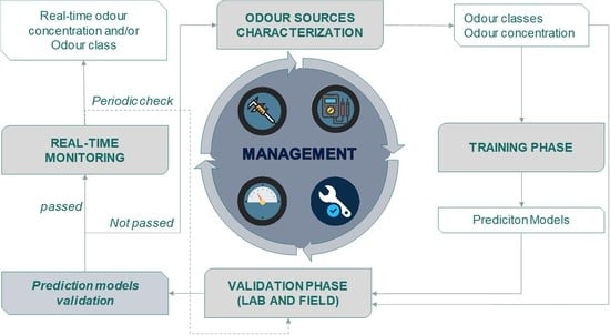
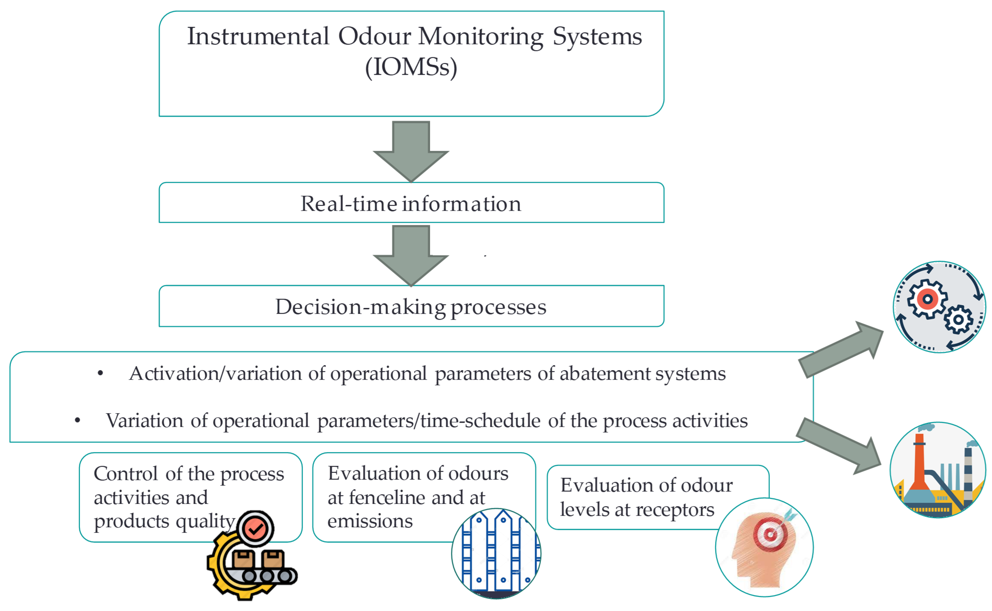
27]. For a specific application, the design of the hardware components of the device and the selection of the most suitable sensors, as well as the methods of feature extraction and classification, are fundamental elements to optimize. The IOMS can be implemented to obtain real-time information needed to support the decision making processes, with a proactive approach and to control the performance of the processes (
Figure 1) [
28,
29]. However, even if it is difficult to implement at an industrial scale, synergistic approaches based on chemical characterization, dynamic olfactometry, and electronic noses have been demonstrated to have the best performances to characterize odors, evaluate their concentration and to develop innovative and tailored monitoring systems [
30]. With these approaches, it is indeed possible to integrate and validate the monitoring results obtained with IOMS with a comprehensive point of view [
31,
32].
The operating phases of an IOMS are generally: training, validation, measurement and management [
27,
33,
34]. Despite the many advantages associated with IOMSs, they still have limitations, such as the difficulty in stabilizing the operating temperature of the devices, the marked dependence of the sensor resistances on operating parameters (temperature, flow rate entering the measurement chamber, humidity, etc.), and possible difficulties in the classification procedure following an improper choice of the method of feature extraction [
35]. The challenge of research is therefore to find answers to these critical issues.
The study is aimed at the development of an advanced IOMS applied for environmental odour monitoring in ambient air, with the objective of overcoming some of the above-mentioned limitations. The experimental analyses have been carried out by considering the operational phases of the IOMS. Optimization of the classification performance has been reported and highlighted by introducing innovative management systems to stabilize the temperature inside the chamber. Moreover, it has been proposed a smart approach able to automatically process the raw data acquired by the sensors to consider temperature fluctuations, which may occur for unfavourable operating conditions. The temperature inside the chamber significantly affects the values detected by the sensors [
36]. It has been extensively demonstrated that under constant gas composition and concentration, the sensor responses change with the variations of temperature and humidity and consequently different methods have been proposed [
37,
38]. The novel proposed approach was designed by experimentally retrieving the correlation curves between temperatures and resistances for the calculation of specific corrective factors. The results demonstrated a significant improvement in terms of recognition performances by applying the proposed approach for the classification of real odour sampling.
2. Materials and Methods
2.1. IOMS Device
The IOMS device was developed by the research group of the Sanitary Environmental Engineering Division (SEED) of the University of Salerno in collaboration with the SPONGE (
www.spongeitalia.com; accessed on 15 June 2021) and SARTEC (
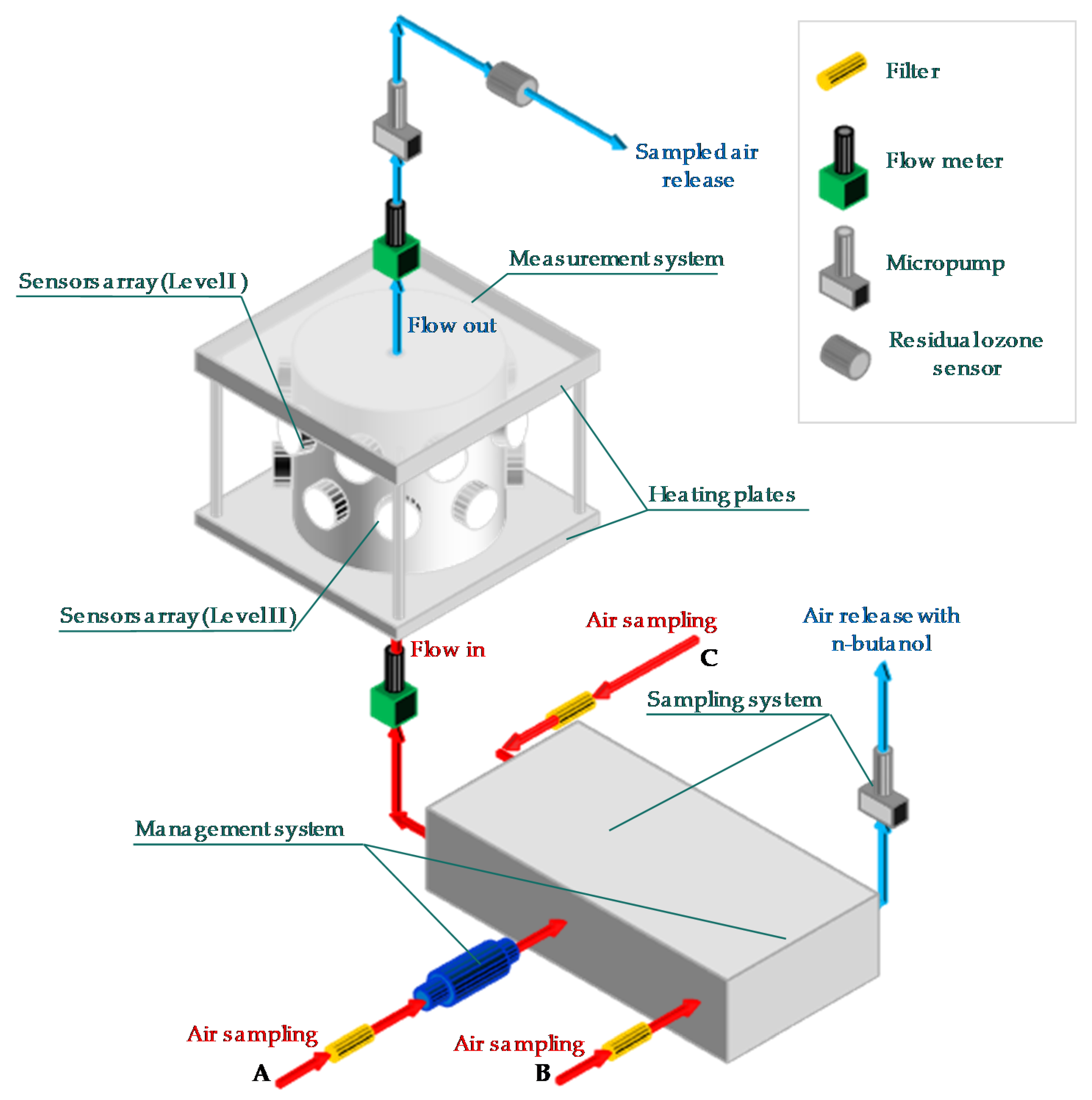
www.sartec.it; accessed on 15 June 2021) companies. The developed IOMS is equipped with integrated management, cleaning and calibration systems which allows its automatic use and application even in particularly aggressive environments for prolonged periods. The hardware component of the IOMS system consists of four main units: sampling, measurement, elaboration and management (
Figure 2). The sampling component consists of membrane pumps and electronic valves designed to convey the sampled gas at a constant flowrate of 300 mL min
−1 in the measuring chamber. The measuring chamber, called CODE, designed and patented by the SEED research group, is equipped with 16 measurement sensors arranged on two levels (
Table 1) and has an internal volume of 300 mL with a residence time of 1 min. The management unit is composed of systems capable of generating zero air and span air. The elaboration unit, composed by a CPU Board and a Main Board, allows the storage, process, and display of the data acquired by the sensors. The IOMS is equipped with a specific software able to work with five different operating modalities (Baseline, Calibration, Training, Validation, Real Time) [
1].
2.2. Experimental Analyses
Four real odour classes were trained for the experimental analysis, sampled at a refining plant (“RF”), from the organic fraction of municipal solid waste (“OF”), coffee aroma (“CA”), and ambient air (“AA”), by using the static lung-effect sampler and 7 L Nalophan bags. The lung-effect sampler (length 730 mm, diameter 160 mm) used has a volume of 10 L, a filling time of 30 to 60 s and a maximum vacuum output of 500 mbar. The systems allowed to collect odour samples in gas sampling bags besides hindering the odour samples contamination. A total of 146 samples were taken.
Table 2 shows the numerical distribution of the total collected samples in the different odor classes.
The samples were then connected to the IOMS for the acquisition. 138 samples were used to create the Training Set (TS), while the remaining 8 (2 for each class) were used as Validation Set (VS). The preliminary validation was performed on TS and on the whole set of samples (TS + VS).
2.3. Elaboration of the Classification Predicitve Model
The Linear Discriminant Analysis (LDA) was used for the creation of the predictive classification model. The LDA approach belongs to the supervised methods [
39,
40]. The elaboration of the prediction models has been implemented with a specific function of the software developed for the IOMS applications [
41].
The sensor array generated a vector of resistance every TA seconds for TF minutes and so it gave as output n vectors of m components, where:
m is the number of the sensors;
TA (Acquisition time) is the time between two different acquisition of resistance equal to 2 s;
a is the number of acquisition;
TF (Flushing duration) is the acquisition time between which the values of resistances were taken in consideration for the calculation of the average value equal to 3 min.
For each sample, the software automatically created a Response Matrix “R” (axm) with the data recorded by the MOS sensors. These matrixes have been preprocessed with the following equation according to a previous study [
1].
For each pre-processed matrix, a vector per sample was extracted by calculating the average of the values per columns. In this way, for each sample of the Training Set, a vector was automatically generated by the SW. The Feature Extraction (FE) matrix contained a vector for each sample of a Training Set (TS).
The matrixes with the preprocessed data (one vector for each sample of the TS) and the vector with the corresponding odour classes (one value for each sample) were analysed with the LDA method according to [
42]. The LDA statistical procedure was implemented returning in output the vectors of the coefficients of the predictive classification model, the confusion matrix, and the Mahalanobis distances.
2.4. Analysis of the Influence of the Temperature on the Sensors Detected Values
The influence of the variation of the detected temperature inside the CODE chamber and the resistance values of the 14 measurement sensors has been evaluated statistically during the acquisition phase. For the TS + VS datasets, for each odour class, correlation graphs were elaborated, implementing linear interpolation analyses. For each sensor, the R-squared coefficient of the correlation curves Temperature–Resistance was calculated according to [
43]. The corrective coefficients were calculated for the sensors, which showed a R-squared coefficient higher than 0.7.
2.5. Optimization Studies and Performance Evaluation
In order to improve the accuracy of the classification predictive models, the set of corrective coefficients obtained by analyzing the temperature influence was applied to the raw resistance data of the measurement sensors. These coefficients were used only for sensors in which the relationship between T and R showed a correlation coefficient higher than 0.7.
To calculate the corrective coefficients, it has been implemented the following algorithm:
- (a)
Calculation of the interpolation curves equations Ri,j = aj Ti,j + bj (where Ri,j are the resistance values, Ti,j the corresponding temperature and aj and bj are the linear combination coefficients different for each j-esimo sensor);
- (b)
Calculation of the benchmark values at 50 °C, for each sensor, using the corresponding equation of the interpolation curves (R50: reference value at temperature of 50 °C);
- (c)
Calculation of the reference values for each value of temperature between 40 °C and 60 °C and for each sensor, using the corresponding equation of the interpolation curves (RTk: reference value at temperature Tk (40–60 °C));
- (d)
Calculation of the corrective coefficients as the ratio between the RTk and R50, different for each j-esimo sensor and for k-esimo Temperature.
The obtained corrective coefficients have been automatically applied at each values of resistance according to the mean value of the temperature measured inside the chamber in the acquisition time.
To quantify the effectiveness of the proposed approach, the performance of the classification prediction model was calculated and evaluated by defining the indicators listed below [
44].
- -
l = number of the classes;
- -
tpi = true positive, represents the number of gaseous samples of the i-class correctly recognized in the i-class;
- -
tni = true negative, represents the number of samples of a different class correctly recognized out of the i-class;
- -
fpi = false positive, represents the number of samples of a different incorrectly attributed to the i-class;
- -
fni = false negative, represents the number of samples of the i-class attributed to a different class.
For an individual class Ci, the assessment is defined by singular accuracy, precision, and recall. Conversely, the quality of the overall classification has been assessed as the sum of counts to obtain cumulative tp, fn, tn, fp (micro-averaging).
3. Results and Discussion
3.1. Predicitve Model for Odour Classification
Table 3 reports the confusion matrix obtained by processing the data of the TS for the creation of a classification model. Results showed a recognition of 127 samples out of 138, equal to 92.0% of correct classification rate.
According to the study of Mahmodi et al. [
45] the obtained prediction model was applied to the TS + VS dataset to verify the influence on unknown samples on the model accuracy (
Table 4). Results show that the samples misclassified resulted in the same both for the TS and TS + VS dataset, while the correct classification rate resulted in being equal to 92.5%.
3.2. Influence of the Internal Temperature on the Measured Values of the Sensors in Terms of Resistance
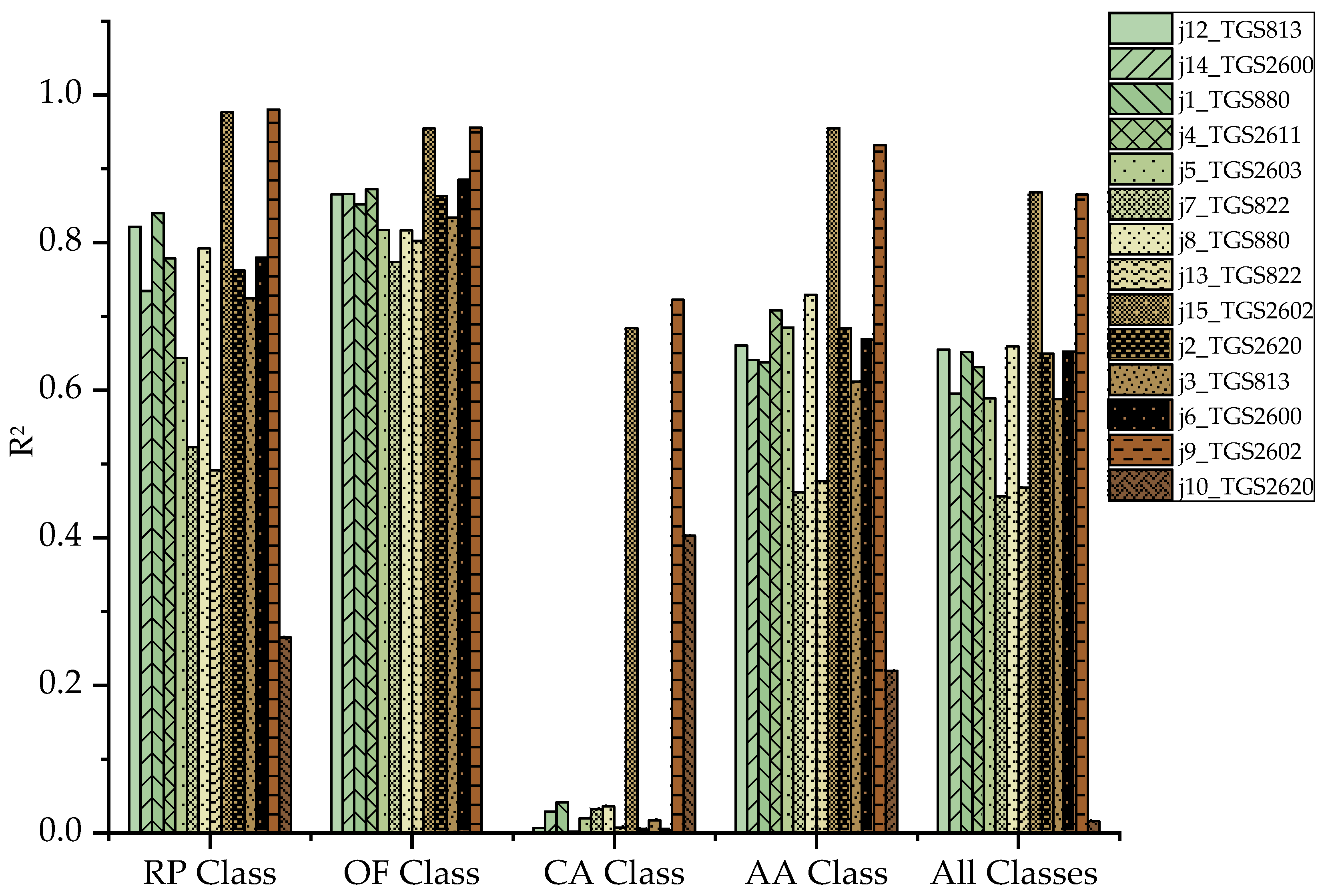
Figure 3 reports the values of the R
2 correlation coefficients between the chamber temperature and the sensors values in terms of electrical resistance, detected inside the measurement chamber, for each odor class, by considering the TS + VS dataset.
Table 5 shows the averages and standard deviation values of the acquisition temperatures of the samples of the TS + VS acquired.
Comparing the resistance values of the single acquisitions, for each class and for each sensor, with the corresponding acquisition temperature a relationship of inverse proportionality between the temperature (T) and the resistances (R) has been confirmed [
46].
For all the investigated classes, the two TGS2602 sensors (Figaro, Arlington Heights, IL, USA) showed R2 coefficients higher than 0.86, except for samples of “CA” class. For “CA” class, in fact, the resistance values resulted in less being affected by the temperature fluctuation, since the lowest variation of the acquisition temperature was among the samples.
Even if the correlation curves have been calculated also for the different odour classes separately, to avoid the influence of the specific conditions on the model results the corrective factors were calculated considering all the samples together. For all the classes, the sensor that demonstrated the lowest R2 value resulted the sensor j10_TGS2620. The TGS2620 sensor is present at both levels (j2_TGS2620—Level I, j10_TGS2620—Level II), with a different conditioning of the resistances. Consequently, the dependence of the sensor on the operating temperature resulted almost negligible for the sensors at the channel j10 (II level) since the lower sensitivity of the sensor to the electrical signals. Conversely, the sensors TGS2602 showed high R2 for all the investigated class.
3.3. Optimization of the Classification Models and Performance Parameters
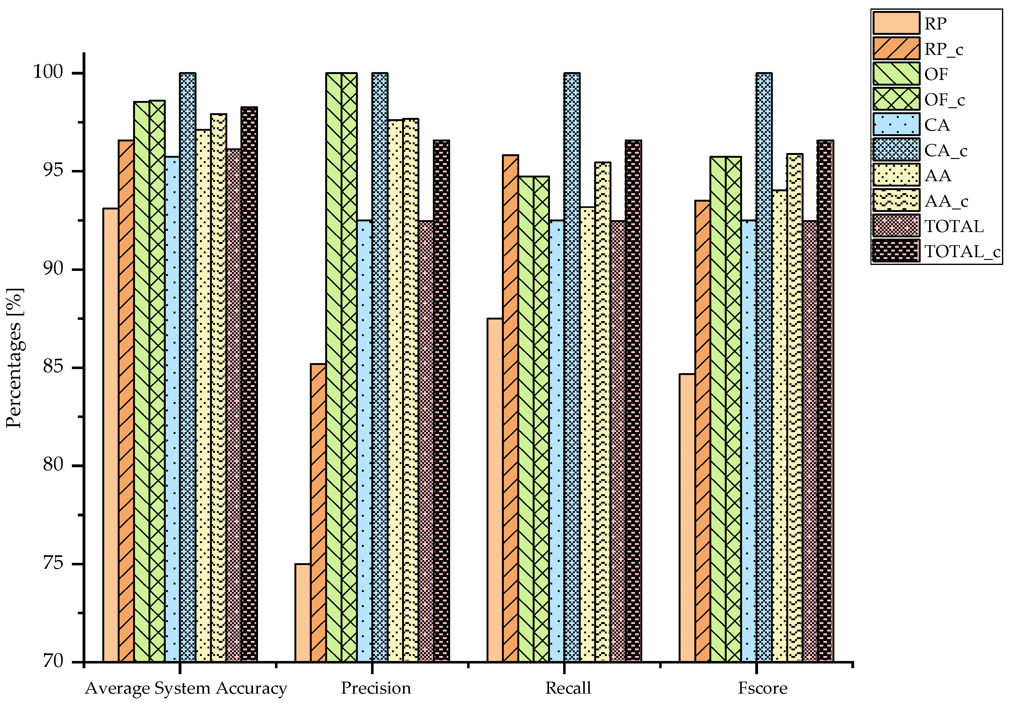
In
Table 6, the confusion matrix obtained by applying the prediction model to the TS + VS samples after the application of the correction coefficients was reported.
The results in terms of accuracy performances have been reported in
Figure 4, in which the performance indicators have been calculated per class for the TS + VS dataset before and after the application of the corrective factors.
Applying the corrective coefficients to the raw data of the 146 samples (TS + VS Set), a significant improvement in terms of recognition performance was obtained. In fact, according to the results of the confusion matrix reported in
Table 5, the misclassified samples decreased from 11 to 5. The results have been confirmed in the graph in
Figure 4, in which a remarkable improvement in terms of classification performances mainly for RP and CA odour classes can clearly be observed.
The strong dependence of almost all sensors on the operating parameters has been indeed reduced by considering the actual acquisition temperatures. The highest accuracy was detected for the OF class, for which, by applying the corrective coefficients, an accuracy of 98.6% was obtained. The overall accuracy increased from 96.1% to 98.3%. All the classes, after the application of the afore-mentioned coefficients, showed accuracies over 96%.
4. Conclusions
The possibility to continuously monitor all the parameters that can affect the operating modes of the IOMS system and their results is a fundamental element to increase the model prediction results and performances. In the present study, the temperature of the gaseous flux in the measurement chamber was highlighted as an important variable to be monitored continuously, given their influence on the values detected by the IOMS sensors. The work also provided a useful methodology experimentally validated to reduce the influence of operating conditions, in terms of temperature and consequently humidity, on the model performances. Corrective factors have been retrieved by analysing the dependence of resistance values on temperature, by optimizing an algorithm automatically applied. The automatic application of corrective coefficients, calculated with dedicated software thus proved to be a useful tool for increasing the reliability of the predictive model, since in the conditions investigated the accuracy of the model increased from 96% to 98%.
The study promotes the development of flexible and robust IOMS devices, with highly adaptable architecture and dedicated software, capable of continuous analysis of all operating parameters and taking them into account in measures to overcome the current limitations in monitoring environmental odours.


 ,
, 


