Abstract
This research describes experiments using LSTM, GRU models, and a combination of both to predict floods in Semarang based on time series data. The results show that the LSTM model is superior in capturing long-term dependencies, while GRU is better in processing short-term patterns. By combining the strengths of both models, this hybrid approach achieves better accuracy and robustness in flood prediction. The LSTM-GRU hybrid model outperforms the individual models, providing a more reliable prediction framework. This performance improvement is due to the complementary strengths of LSTM and GRU in handling various aspects of time series data. These findings emphasize the potential of advanced neural network models in addressing complex environmental challenges, paving the way for more effective flood management strategies in Semarang. The performance graph of the LSTM, GRU, and LSTM-GRU models in various scenarios shows significant differences in the performance of predicting river water levels based on rainfall input. The MAPE, MSE, RMSE, and MAD metrics are presented for training and validation data in six scenarios. Overall, the GRU model and the LSTM-GRU combination provide good performance when using more complete input variables, namely, downstream and upstream rainfall, compared to only using downstream rainfall.
1. Introduction
Flooding is one kind of natural disaster that commonly affects many different nations, including Indonesia. Flooding is a common hazard for local villages in Semarang City, especially in the East Flood Canal River basin. Heavy rainfall in upland and downstream locations can affect river water levels, potentially leading to flooding [1,2]. Therefore, predicting river water levels is very important for disaster mitigation and emergency response planning.
In Semarang City, especially in the East Flood Canal River basin, floods often occur, caused by high rainfall in the upstream and downstream areas. Currently, because river flow dynamics and rainfall patterns are so unpredictable, precise water level estimates are difficult to achieve. There is insufficient time to prepare for and respond to floods when there is no trustworthy forecast system in place, which can cause significant losses for nearby towns.
Over the past two decades, numerous machine learning and AI-based techniques have been applied to hydrological modeling and forecasting. Traditional methods include statistical models and simpler machine learning algorithms. However, with the advancement of technology, more sophisticated approaches have emerged. For instance, adaptive neuro-fuzzy systems have been explored for water level forecasting due to their ability to model complex non-linear relationships and adapt to new data. Specifically, Hong and White (2009) demonstrated the use of a dynamic neuro-fuzzy system with an online and local learning algorithm for hydrological modeling [3], while Nguyen et al. (2018) employed neuro-fuzzy models with local learning for water level forecasting [4].
The utilization of advanced technology and techniques, such as deep learning, can greatly assist in the prediction of river water levels in this digital age. Combining gated recurrent unit (GRU) and long short-term memory (LSTM) is one deep learning technique that can be applied [5,6,7]. Both models are known for their adept handling of time series data and for their ability to remember important details from historical data, which is particularly pertinent when discussing water.
The use of deep learning technology in predicting river water levels will not only increase prediction accuracy, but it will also provide deeper insight into rainfall patterns and river flow dynamics [8,9,10]. Deep learning is a branch of machine learning that emphasizes using large, deep artificial neural networks to model and understand patterns in data. Some algorithms that are often used for prediction are long short-term memory (LSTM) and gated recurrent unit (GRU), which have been confirmed impactful in time series data analysis because of their ability to handle temporal dependencies [11,12,13]. However, each model has advantages and disadvantages. LSTM excels at remembering long-term dependencies. It is designed to overcome the long-term dependency problem that RNNs often face when long sequence data are processed. In recent years, LSTM has achieved great results in various fields, including speech recognition, natural language processing, and time series prediction. LSTM is a great method in for prediction, which is a typical prediction in time series problems [14,15]. Flood prediction requires continuous understanding and processing of hydrological data, such as rainfall and river water levels, which form the contexts for future flood predictions. The structure of LSTM, which is able to overcome and remember the dependencies of long-term sequential data, makes it an ideal choice for this problem [16,17,18,19]. The use of LSTM models in flood prediction is steadily increasing. Early research mainly concentrated on using LSTM to build a model and conduct prediction using rainfall and river water levels at various locations [20]. In deep learning technology advances, researchers have begun to explore more elaborate models, such as integration between convolutional neural networks (CNNs) and LSTM, to process hydrological data from various geographic regions, improving the precision and accuracy of flood predictions [21,22,23].
Gated recurrent unit (GRU) integrates a gate mechanism that allows selective updating of its hidden state as input data. In particular, GRU operates an update gate that integrates the purpose of the forget gate and input gate in LSTM, simplifying the architecture and reducing the number of parameters. This results in efficiency in computation and faster training times. The GRU design combines hidden cells and states, improving the efficient flow of information. This allows the GRU to retain important information while discarding irrelevant ones, making it a very appropriate data analysis sequence [24,25,26,27,28,29,30].
In recent years, the GRU model has been investigated for flood prediction. GRU shows superior performance for short-range flood forecasting in comparison to other algorithms, especially LSTM [27]. However, the GRU model requires improvement for long-term forecasting [28,29]. Compared with other RNN models, the GRU architecture is simpler with fewer gate mechanisms, making it more computationally efficient [30]. GRU has comparable performance to LSTM in a variety of machine learning tasks, including sequence prediction. GRU has shown promising results in practical uses, such as speech recognition, location prediction, time series forecasting, and dynamic risk prediction in healthcare. Additionally, GRU has been explored with other models, such as convolutional neural networks (CNNs), to improve performance in tasks, such as electrical load estimation. The GRU model was chosen in this analysis because of its superiority in weather prediction. GRU has been widely used in various domains, including landslide displacement prediction, traffic prediction [31], electricity load estimation, solar radiation estimation [32], precision agriculture [33], wind speed and temperature estimation [34], carbon dioxide concentration prediction [35], and solar radiation estimation [36]. The GRU model has exhibited encouraging outcomes concerning precision, predictive capability, and efficiency across diverse meteorological forecasting assignments, rendering it a favorable selection for this examination.
Previous studies have explored various machine learning models for flood prediction, though many struggle with accurately handling multi-variable time series data and long-term dependencies. Existing models often either oversimplify the problem or fail to integrate the advanced techniques effectively. This study introduces a hybrid model combining LSTM and GRU networks to enhance flood prediction accuracy. By integrating these advanced deep learning techniques, we aim to improve the handling of complex, multi-variable time series data and better capture long-term dependencies. Our innovative approach leverages the strengths of both LSTM and GRU models to provide more accurate and reliable flood predictions, offering valuable insights for disaster mitigation and decision-making in Semarang. This work fills a critical gap in current flood prediction methodologies and provides a practical framework for integrating IoT-based time series data into predictive models.
In this research, rainfall data from two different points, namely, rainfall in the upstream area (Rainfall 1) and in the downstream area (Rainfall 2) of the East Flood Canal River flow in Semarang, were used as the main variable. We utilized these data with multiple variables, so the LSTM-GRU model is expected to be able to predict water levels with high accuracy [37,38]. These accurate predictions will later be able to help the authorities take appropriate preventive steps and minimize the impact of flooding that occurs.
This study aims to combine LSTM and GRU in a hybrid model for flood prediction in Semarang using IoT-based time series data. By integrating these two methodologies, it is hoped that the resulting model can provide more accurate and reliable predictions, thus helping the government and society take more effective preventive measures.
2. Materials and Methods
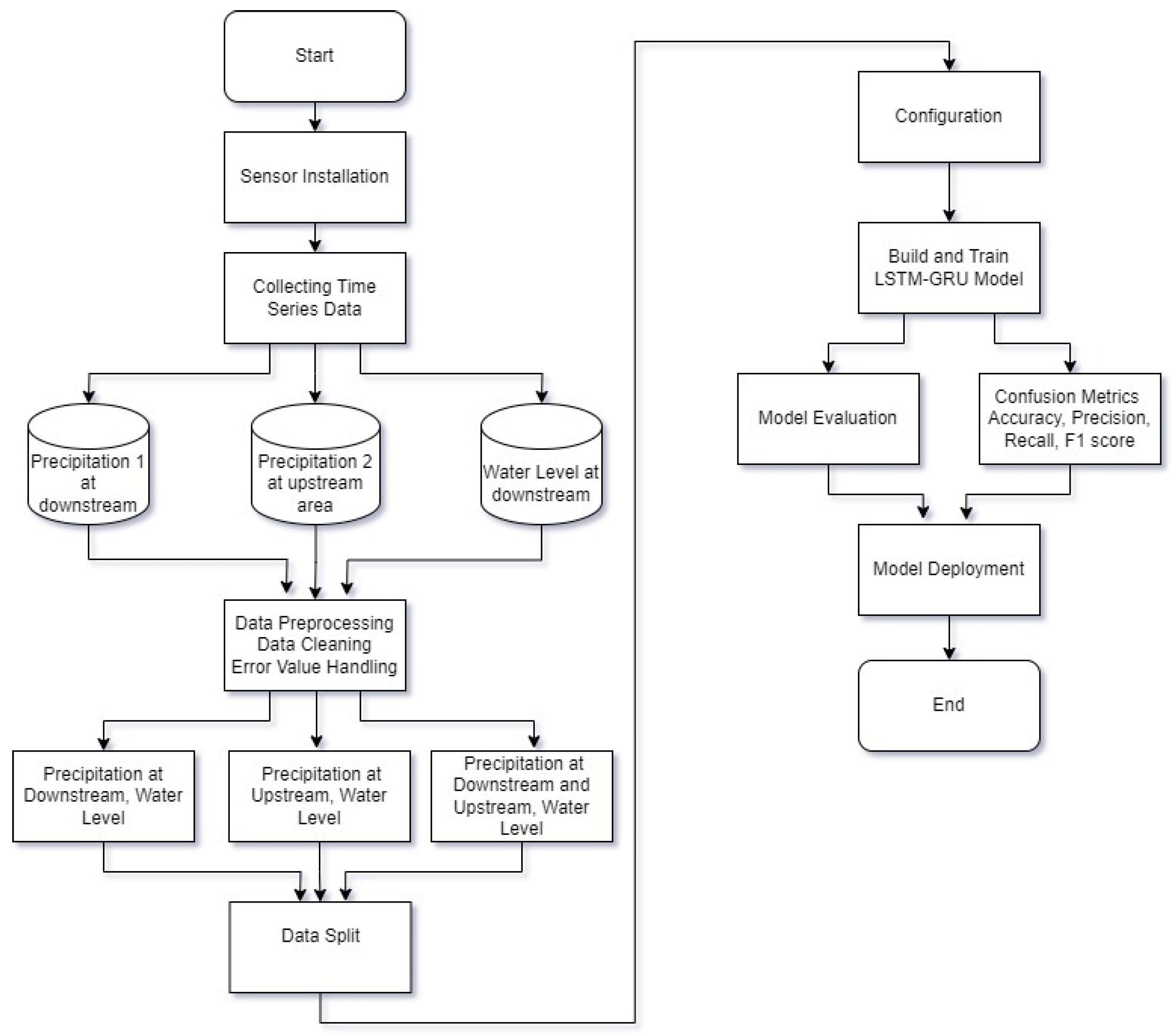
This section describes the proposed model and algorithm used in this study, along with the procedures for data collection and processing. Collected data included Precipitation (rainfall) 1 at the downstream area located around East Flood Canal River, and Precipitation 2 at the upstream area located around Pucanggading Dam. Data were then processed in three scenarios using LSTM, GRU, and a combination of both. Then, the model was evaluated using MAPE, MSE, RMSE, and MAD. The model was also evaluated using the confusion matrix to demonstrate the effectiveness of the classification model. Figure 1 illustrates the research techniques used to accomplish this objective.
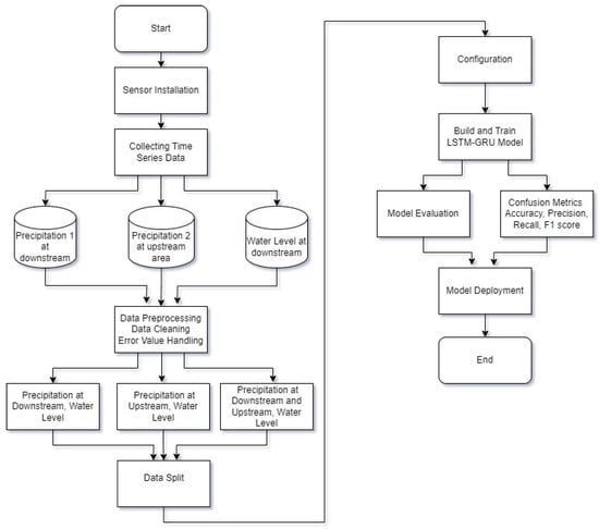
Figure 1.
Flowchart of the research process.
2.1. Study Area
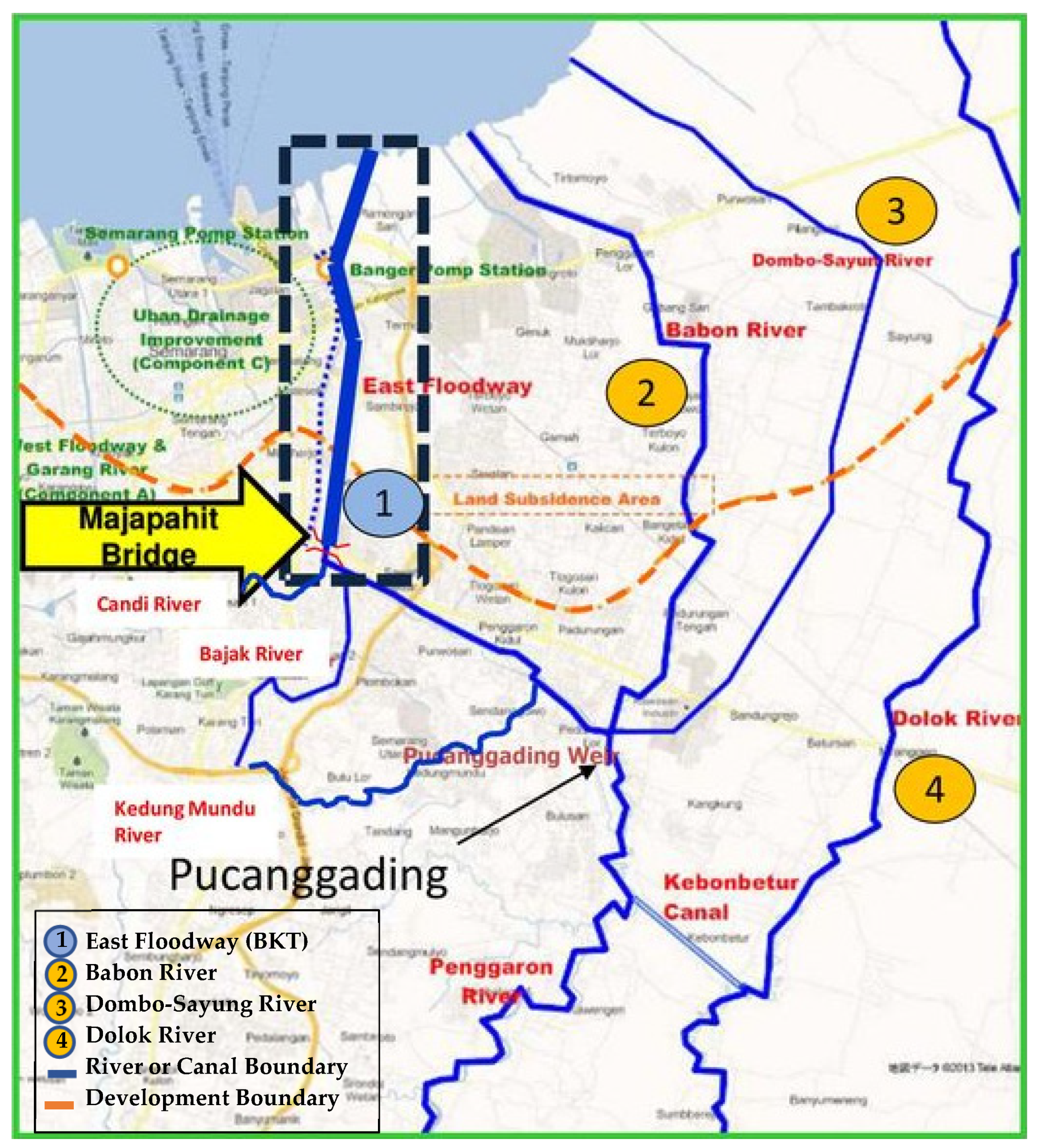
This research was conducted in the eastern city of Semarang and parts of Demak Regency, which are often hit by floods due to high rainfall and sea tides. Pucanggading Dam was built on the Dolok Penggaron river system. The weir gets its water supply from the Penggaron River and the Dolok River, then through the weir the water is distributed to three branches, namely, the East Flood Canal River, Babon River, and Dombo Sayung River. Therefore, adjustments to the design of the weir and other additional buildings, as necessary, are made. The Penggaron River and Dolok River are the origins of water that flows into several rivers downstream, some of whose overflows cause flooding. The Penggaron River is divided into three rivers from upstream Pucanggading, namely, the East Flood Canal/Banjir Kanal Timur (BKT), the Babon River, and the Dombo-Sayung River. Initially, only the Babon River was connected to the Penggaron River as the downstream part of the river, but to control the flooding of the Penggaron-Babon River, the East Flood Canal (BKT) was artificially connected to the Penggaron River in Pucanggading. Then, the Dombo-Sayung River was recently connected to the Penggaron/Babon River in Pucanggading as another canal flood route from the Penggaron River. Apart from controlling the flooding of the Dolok River, the Kebon Batur River was built as a flood bridge from the Dolok River to the Penggaron River upstream of Pucanggading. An overview of the river basin map in Semarang is shown in Figure 2. Point 1 represents the BKT: Detailed Design (D/D) Stretch, point 2 identifies the Residential Area or Land Subsidence Area, point 3 denotes the Dombo-Sayung River, and Point 4 marks the Dolok River. Additionally, the caption specifies the color coding used in the map: the blue line illustrates the River or Canal Boundary, whereas the orange line indicates the Development Boundary or Planned Area.
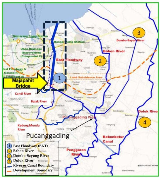
Figure 2.
Study area map.
2.2. Data Collection
Data collection was a crucial stage in this research, using a combination of LSTM and GRU. For this research, we collected data from two main locations, namely, the Pucanggading Dam (upstream) and the East Flood Canal River basin (downstream). The main focus was on measuring water levels in the downstream area. Automatic water level sensors and rainfall sensors were installed and connected to an IoT network to monitor water level changes in real time. This sensor sent periodic data every 15 min, recording small and large changes in the dam’s water level. These data are very important for identifying water flow patterns from upstream to downstream, which was an early indicator of potential flooding. For data collection in the East Canal Flood Watershed (downstream), rainfall sensors and water level sensors were also installed. Rainfall sensors record the intensity and duration of rain in the area, which was a critical factor in analyzing potential flooding. Water level sensors were installed at several points along the river to monitor rising water levels due to heavy rain. Data from these two locations were sent to a central server in real time, enabling continuous monitoring of water conditions. Integration of data from upstream and downstream provided a comprehensive picture of water dynamics in the region. These data were then used in a prediction model that combines LSTM and GRU, which was expected to provide more accurate flood predictions and assist in decision-making for flood risk mitigation. The dataset under examination comprised a total of approximately 1772 records, meticulously collected over a defined period. This dataset included periodic measurements taken every 15 min from both upstream and downstream locations, allowing for a comprehensive analysis of water levels and rainfall intensities. Table 1 summarizes the key statistical information derived from the dataset.

Table 1.
Summary statistics for water levels and rainfall intensity.
During the data collection period, there were 32 recorded instances of rainfall and 9 occurrences of flooding in areas known to be prone to such events. This highlighted a notable correlation between heavy rainfall and flooding occurrences, underscoring the vulnerability of these regions to flood events.
In summary, the data provided valuable insights into the water levels and rainfall intensities both upstream and downstream. The variations and averages observed revealed important patterns and potential implications for water management and flood risk assessment in the studied areas.
After data were collected through the sensors, the next step was creating the scenarios. The aim of the scenarios was to compare the performance of flood prediction models (LSTM, GRU, and LSTM-GRU) with different contextual data: downstream rainfall, upstream water levels, and upstream rainfall. Each scenario evaluated whether adding upstream rainfall data would improve the prediction accuracy. The results would determine the most effective model for an early-warning and flood mitigation system. In Scenarios 1–3, LSTM and GRU evaluated predictions with downstream rainfall data and upstream water levels, while Scenarios 3–6 added upstream rainfall data to see whether the accuracy increased. The LSTM-GRU scenario tested the hybrid model with the same data. The ultimate goal was to conclude the most effective model for increasing the accuracy of flood predictions, which will be used for early-warning and disaster mitigation systems. Table 1 shows the details of the experiment.
Table 2 provides a detailed comparison of different scenarios for predicting downstream water levels using different machine learning models and input variables. Specifically, Scenario 1 (S1) used an LSTM model with downstream rainfall data to predict downstream water levels, while Scenario 2 (S2) applied a GRU model with the same input data. Scenario 3 (S3) explored a hybrid LSTM-GRU model using only downstream rainfall. In contrast, Scenario 4 (S4) tested an LSTM model with both downstream and upstream rainfall data to predict downstream water levels. Similarly, Scenario 5 (S5) used a GRU model with both rainfall sources, and Scenario 6 (S6) combined LSTM and GRU models with both downstream and upstream rainfall inputs. These settings were designed to assess the impact of incorporating upstream rainfall data and using different model architectures on the accuracy of downstream water level prediction.
Table 2.
Details of experiments.
2.3. Training and Testing Data
After the data were collected and normalized, they were split into a training and a test dataset. This data split was performed to ensure that the model could be properly evaluated on data that have never been seen before. Data were divided by a certain ratio, a training split of 80% and a testing split of 20%. The data were split randomly to ensure that the data in the training set and test set were representative.
2.4. LSTM Model Development
In this phase, we utilized LSTM to construct the model. LSTM is a kind of artificial neural network that is suitable for time series data processing and complex pattern detection in the data. In the case of DDoS attack detection, network data are often sequential and have temporal dependencies. LSTM is very effective in handling these types of data because of its ability to remember information over long and short periods of time. Below is an explanation of how each LSTM formula is used in this context:
- Input gate:
: A sigmoid activation function that converts the input value to a range between 0 and 1.
: Weights used in input gate calculations.
: Hidden state from the previous timestep, which contains information from previous steps and helps predict next steps.
: Input at timestep ; in this context, is the rainfall data at time , which includes Rainfall 1 and Rainfall 2. For example, in this case, is [20,23].
Example: is the input to the timestep with values of 23 and 20, and is the hidden state of the previous timestep. Suppose: For the initial hidden state and cell state, that means = 0 and = 0, then ). Assumption: is [0.5,0.5] and is 0; then, = (21.5) ≈ 1.
- 2.
- Forget gate:
: Weights used in forget gate calculations.
: Bias used in forget gate calculations.
Example: If is the input to the timestep with values of 23 and 20, ). Assumption: is [0.5,0.5] and is 0; then, = ≈ 1.
- 3.
- Candidate gate:
: Candidate cell state, namely, the resulting new value that can be added to the cell state.
: Weights used in candidate gate calculations.
: Bias used in candidate gate calculations.
Example: If is the input to the timestep with values of 23 and 20, . Assumption: is [0.5,0.5] and is 0; then, ≈ 1.
- 4.
- Cell state update:
: Candidate value for the new cell state at time t.
Cell state updates combine information from the forget gate, input gate, and candidate cell state.
The cell state update value can be calculated as: .
- 5.
- Output gate:
: Output gate, which decides which value from the cell state will be passed to the hidden state.
: Weights used in forget gate calculations.
: Bias used in candidate gate calculations.
Example: If is the input to the timestep with values of 23 and 20, then = = ≈ 1.
- 6.
- Hidden state:
: Hidden state updated at timestep , which generates new output based on the updated cell state.
The hidden state value can be calculated as: ∗ tanh () = 1 ∗ tanh (1) ≈ 0.76.
2.5. GRU Model Development
The GRU (gated recurrent unit) makes use of a gate mechanism to limit the flow of information within the network. It is designed to ensure that the temporal dependencies in time series data can be captured. This example shows how the concealed state is updated based on the input rainfall and water level at every interval. Training will optimize features, such as weights and bias, in practical implementation to produce predictions that are more accurate. The upcoming water levels can then be predicted using the GRU-built model based on rainfall data collected in real time.
- Reset gate:
- : Reset gate, which controls how much information the previous hidden state, , contains that will be forgotten.
- : A sigmoid activation function that maps input to a range between 0 and 1.
- : The weight matrix used to multiply input data, , in the reset gate.
- : Hidden state from the previous timestep.
- : Input vector at timestep .
- : Bias vectors are added in the reset gate.
- 2.
- Update gate:
- : Update gate, which controls how much information from the previous hidden state, , will be taken to the current hidden state ().
- : Bias vectors are added in the update gate.
- 3.
- Candidate activation:
- : Candidate activation, where new information is generated for the current hidden state.
- : The weight matrix used to multiply candidate activation, , in the reset gate.
- : Hidden state from the current timestep.
- : Bias vectors are added in candidate activation.
- 4.
- Cell state update:
- : Current hidden state, which is a combination of the previous hidden state, , and the candidate activation, , which is controlled by the update gate, .
The proposed model integrates both long short-term memory (LSTM) and gated recurrent unit (GRU) networks to capture complex temporal dependencies and improve the prediction accuracy. The LSTM and GRU layers were stacked sequentially to form a hybrid architecture, where the LSTM layer processes the input sequence first, followed by a GRU layer that further refines the learned features. Specifically, the LSTM layer with 64 units was used as the first layer, followed by a GRU layer with 32 units. The outputs from both LSTM and GRU layers were concatenated and fed into a dense layer for final prediction.
The model was implemented using the Keras library with TensorFlow backend. Each recurrent layer utilized a ReLU activation function, and dropout regularization was applied with a dropout rate of 0.2 to prevent overfitting. The combined model was trained using the Adam optimizer with a learning rate of 0.001, and the training was conducted for 100 epochs with a batch size of 64. The choice of stacking LSTM and GRU layers aimed to leverage the strengths of both models: LSTM is known for its ability to learn long-term dependencies, while GRU is computationally efficient and requires fewer parameters, making the model robust and effective.
2.6. Performance of Model Evaluation
In model evaluation, we used confusion matrices to determine model specifications. false positive (FP), false negative (FN), true positive (TP), and true negative (TN) are some components of the confusion matrix. We provided a confusion matrix to demonstrate the effectiveness of our classification model. The confusion matrix shows how valid the predictions were. Additionally, we evaluated our model using metrics frequently used in DDoS. The following are the mathematical formulas for accuracy, precision, recall, and F1-score:
- 1.
The confusion matrix helps in measuring the accuracy of model predictions, namely, how often the model predicts correctly relative to the total predictions made, which is calculated as:
where TP = true positive, TN = true negative, FP = false positive, and FN = false negative.
measures the proportion of correctly classified instances (both true positives and true negatives) out of the total number of instances. In flood prediction, it tells us how often our model correctly predicted whether a flood would occur or not. For example, if our model predicted floods and non-floods correctly 85 out of 100 times, the accuracy would be 85%.
- 2.
measures how many flood status predictions were correct out of all flood status predictions made. High precision indicates that the model rarely gives false alarms. It is calculated as:
where P = precision, TP = true positive, and FP = false positive.
measures the proportion of true positive predictions out of all positive predictions made by the model. In the context of flood prediction, it reflects how often our model’s flood predictions were actually correct. For instance, if our model predicted a flood 30 times and 25 of those predictions were correct, the precision would be 83.3%.
- 3.
measured how many flood events the model was actually able to predict. High recall indicates that the model did not often miss actual flood events. It is calculated as:
where r = Recall, TP = true positive, and FN = false negative.
measures the proportion of actual positives that are correctly identified by the model. In flood prediction, this indicates how well the model identified all actual flood events. If there were 40 actual flood events and the model identified 30 of them, the recall would be 75%.
- 4.
is the harmonic mean of precision and recall, providing an idea of the balance between these two metrics. This is important because it provides a more thorough evaluation of model performance, especially in the context of flood prediction, where both precision and recall are critical metrics. It is calculated as:
where R = and P = .
The is the harmonic mean of precision and recall, providing a single metric that balances both aspects. It is especially useful when the class distribution is imbalanced. For our flood prediction model, if precision is 83.3% and recall is 75%, the F1-score will be approximately 78.2%. This reflects a balance between detecting as many floods as possible (high recall) and ensuring that predictions of floods are accurate (high precision).
In predictive model evaluation, we also used various metrics to assess the accuracy and effectiveness of the predictions generated. These metrics provide important insights into the performance of the model by measuring the deviation between the predicted values and the actual observations. Understanding these metrics is essential for selecting the most appropriate model and improving its predictive ability.
- Mean Absolute Percentage Error (MAPE)
MAPE measures the average model prediction error as a percentage of the actual water level. In the case of floods, MAPE indicates by how much the model was wrong in projecting the water level compared to the actual data. This metric helps assess how well the model predicted water level fluctuations, where the lower the MAPE value, the more accurate the model was in predicting the water level that is likely to cause flooding.
where:
- : Value of the data for period t.
- : Prediction for period t.
- : Number of data points.
- 2.
- Mean Squared Error (MSE)
MSE calculates the mean square of the difference between the predicted water level and the actual water level. In the context of floods, MSE gives an idea of by how much the model was wrong in predicting water levels, with a larger penalty for larger errors. This metric is useful for assessing how much the model deviated from the actual water level, which is important for understanding potential errors in flood forecasting.
where:
- : Actual water level.
- : Predicted water level.
- : Number of data points.
- 3.
- Root Mean Squared Error (RMSE)
RMSE is the square root of MSE, yielding a measure of model error in the same units as the water level. This allows for a more intuitive interpretation of how far the predicted water level deviated from the actual value. In the case of flooding, RMSE helps in assessing how well the model predicted water levels that may indicate potential flooding.
- 4.
- Mean Absolute Deviation (MAD)
MAD measures the average absolute deviation between actual and predicted water levels. It provides a direct indication of by how much the model was wrong, on average, in predicting water levels. For flood disaster prediction, MAD provides a clear indication of how accurate the model was in predicting potential water levels that could cause flooding.
where:
- : Actual water level.
- : Predicted water level.
- : Number of data points.
- 5.
- Mean Absolute Error (MAE)
MAE measures the average absolute error between predicted water levels and actual values. MAE provides a direct measure of model prediction error without penalty for large errors. In the context of flood prediction, MAE helps assess how well a model predicted water levels that are important for flood risk identification.
where:
- : Predicted water level.
- : Actual water level.
- : Number of data points.
- 6.
- Nash–Sutcliffe Efficiency (NSE)
NSE measures how well a model predicts water level variations compared to a simple average model. In the case of floods, NSE provides an idea of how effectively a model explained water level fluctuations that can affect flood risk, compared to simply using the average water level value.
where:
- : Predicted value.
- : Means of actual value.
- : Number of data points.
Interpretation: ranges from −∞ to 1. An value of 1 indicates a perfect model, while an value of 0 means that the model is no better than using the mean of the observed data as a prediction. A negative value indicates that the model is worse than using the mean of the observed data as a prediction.
- 7.
- Coefficient of Determination ()
R2 measures how well a model predicts water level variations compared to the mean water level value. In the context of flooding, indicates the proportion of water level variability that can be explained by the model, helping to assess the strength of the relationship between predictions and actual values.
where:
- : Predicted value.
- : Means of actual value.
- : Number of data points.
Interpretation: ranges from 0 to 1. An value of 1 indicates a model that explains all the variability in the data. An R2 value of 0 means that the model explains none of the variability in the data.
3. Results
In this research, we conducted a series of experiments using LSTM and GRU models, as well as a hybrid approach combining both, to predict floods in Semarang based on time series data.
We first present the performance of the individual models. The LSTM model exceled in capturing long-term dependencies within the time series data, whereas the GRU model was more adept at processing short-term patterns. This differentiation highlights the specific strengths of each model in different aspects of flood prediction.
Next, we describe the performance of the LSTM-GRU hybrid model, which combines the strengths of both LSTM and GRU. Our experiments demonstrated that this hybrid model achieved superior accuracy and robustness in flood prediction compared to the individual models. The hybrid approach benefited from the complementary strengths of LSTM and GRU, resulting in a more reliable prediction framework.
3.1. Training and Validation Results
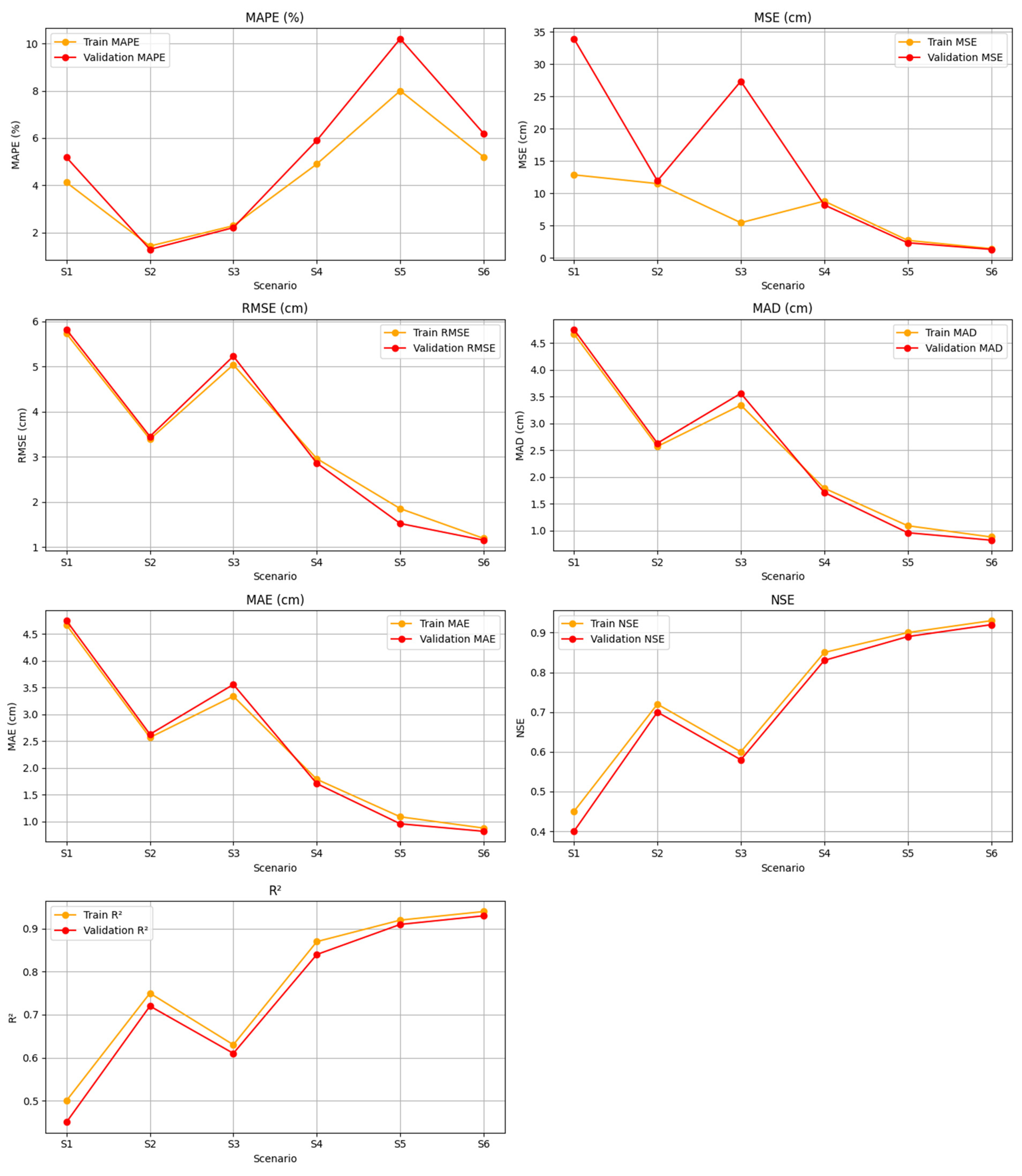
Figure 3 shows a comparison of various evaluation metrics for training and validation models across six different scenarios (S1 to S6). The metrics used included Mean Absolute Percentage Error (MAPE), Mean Squared Error (MSE), Root Mean Squared Error (RMSE), Mean Absolute Deviation (MAD), Mean Absolute Error (MAE), Nash–Sutcliffe Efficiency (NSE), and the Coefficient of Determination (R2). The data illustrate the variation in model performance across scenarios, with the general trend showing an increase in model accuracy across scenarios S4 to S6.
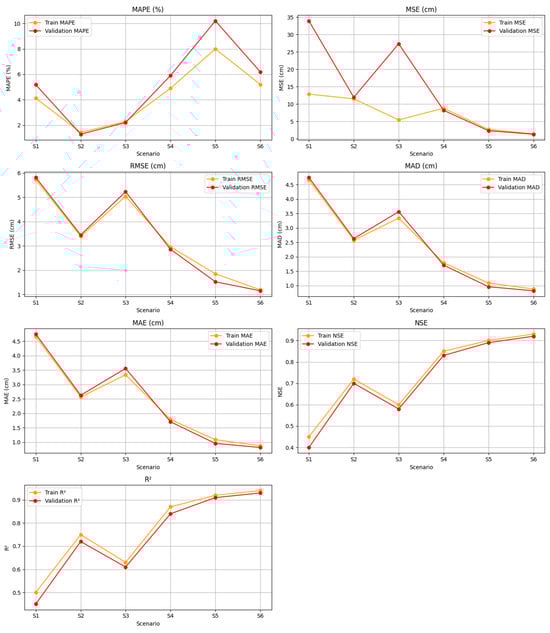
Figure 3.
Performance of LSTM, GRU, and LSTM-GRU models.
Figure 3 shows changes in MAPE, MSE, RMSE, MAD, and MAE values for training and validation data across six different scenarios. Scenario S1 showed quite good performance, while S2 showed improved accuracy in several metrics compared to S1. Scenario S5 showed an increase in MAPE, but there was a positive trend in several other metrics. In contrast, Scenario S6 showed a significant decrease in all metrics, reflecting an increase in consistency and overall model performance.
The NSE graph shows a variation in model performance among the scenarios. Scenarios S2 and S3 showed lower NSE values compared to the other scenarios, indicating that the model’s predictive ability can still be optimized. However, from Scenarios S4 to S6, the NSE values increased consistently, with S6 reaching the highest value for both training and validation data, indicating better model effectiveness in these scenarios.
The R2 graph showed an increase in R2 values from S1 to S6, for both training and validation data. The early scenarios (S1 to S3) showed greater variation, but there was a steady increase from S4 to S6. The high R2 values in the late scenarios indicate that the model had a stronger ability to explain data variability in these scenarios. This increasing trend indicates that the model experienced continuous improvement as the scenarios changed, with the best performance achieved in S6.
Table 3 shows the results of model evaluation using several error and performance metrics, both for training data (Train) and validation data (Val.), in six different scenarios (S1 to S6). The metrics used included MAPE, MSE, RMSE, MAD, MAE, NSE, and R2.
Table 3.
MAPE, MSE, RMSE, MAD, MAE, NSE and R2 values.
In S1, on training data, the MAPE value was 4.12%, MSE was 12.86 cm, RMSE was 5.73 cm, MAD was 4.67 cm, and MAE was 4.67 cm. NSE and R2 were 0.45 and 0.50, respectively, indicating quite low accuracy. For validation data, MAPE reached 5.18%, MSE was much higher at 33.94 cm, and RMSE was 5.82 cm. The NSE and R2 values for validation were also relatively low, at 0.4 and 0.45.
In S2, model performance increased significantly, with MAPE values for training data of 1.43%, MSE of 11.5 cm, and RMSE of 3.39 cm. NSE and R2 also increased to 0.72 and 0.75. Validation data showed similar results with MAPE of 1.29%, MSE of 11.93 cm, and RMSE of 3.45 cm. NSE and R2 for validation were at 0.7 and 0.72, indicating a balance in performance between training and validation data.
In S3, there was a slight decrease in model performance compared to S2. For the training data, the MAPE was 2.29%, MSE was 5.44 cm, and RMSE was 5.04 cm, with NSE and R2 of 0.6 and 0.63, respectively. The validation data had a MAPE of 2.21%, MSE of 27.36 cm, and RMSE of 5.23 cm, and NSE and R2 values of 0.58 and 0.61.
In S4, the model showed significant performance improvement, with a training MAPE of 4.9%, MSE of 8.79 cm, and RMSE of 2.96 cm. NSE and R2 increased to 0.85 and 0.87. Validation also showed improvement, with a MAPE of 5.9%, MSE of 8.19 cm, and RMSE of 2.86 cm, and NSE and R2 of 0.83 and 0.84.
In S5, the MAPE value for training was 8%, MSE was 2.71 cm, and RMSE was 1.85 cm, with excellent NSE and R2 of 0.9 and 0.92. Validation data also showed improvement, with MAPE of 10.2%, MSE of 2.33 cm, and RMSE of 1.52 cm. NSE and R2 values for validation were also high, namely, 0.89 and 0.91.
S6 showed the best performance, with training MAPE of 5.2%, MSE of 1.42 cm, and RMSE of 1.19 cm. NSE and R2 reached 0.93 and 0.94, respectively. Validation also showed optimal results, with MAPE of 6.19%, MSE of 1.31 cm, RMSE of 1.15 cm, and NSE and R2 of 0.92 and 0.93.
Overall, Table 3 shows that the model experienced significant performance improvements from Scenarios S1 to S6, for both training and validation data, with S6 being the most optimal scenario.
3.2. Performance Model Evaluation Using Confusion Matrix
In this research, the main objective was to predict downstream water levels based on rainfall data using various machine learning models, such as LSTM, GRU, and a LSTM-GRU hybrid model. One way to evaluate the performance of this prediction model is to use accuracy, precision, recall, and F1-score metrics obtained from the confusion matrix. By using a confusion matrix, this research could compare the performance of various models and determine which model was most effective in predicting flood status.
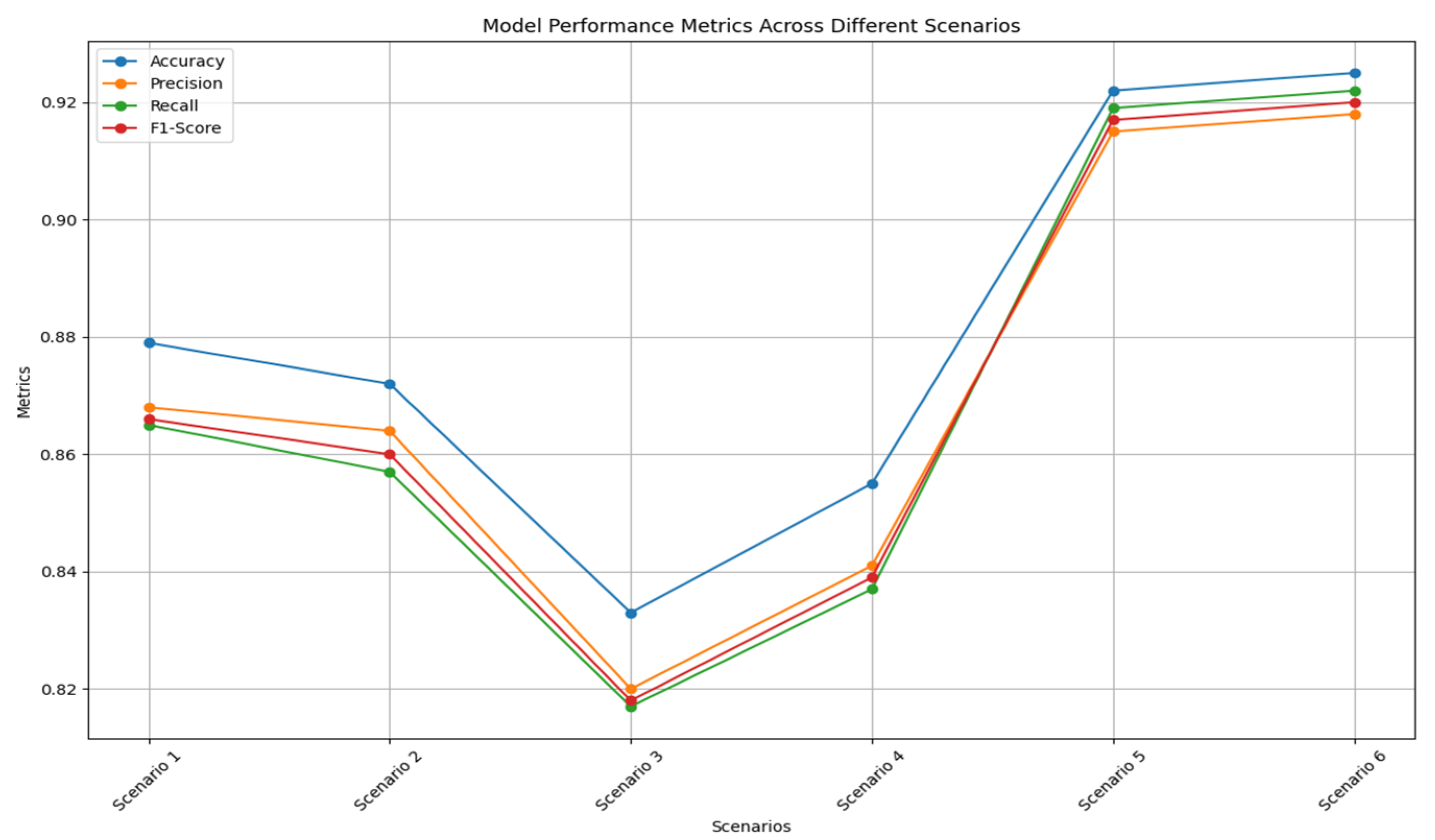
Figure 4 illustrates the performance of the LSTM, GRU, and LSTM-GRU models in various scenarios, showing significant differences in performance in predicting river water levels based on rainfall input using the confusion matrix. This graph presents accuracy, precision, recall, and F1-score metrics for the six different scenarios. On the horizontal axis, there are Scenarios 1 (S1) to 6 (S6), while the vertical axis shows the performance metric values in percentage form. Each bar on the graph represents the accuracy, precision, recall, and F1-score values for each scenario. Overall, this graph shows that the GRU model and the LSTM-GRU combination provided the best performance when using more complete input variables, namely, downstream and upstream rainfall, compared to using only downstream rainfall. These models were able to significantly improve the accuracy and quality of predictions, as shown by the increase in the accuracy, precision, recall, and F1-score values in the graph.
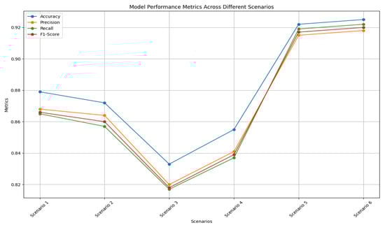
Figure 4.
Performance comparison of LSTM, GRU, and LSTM-GRU models.
In this study, the performance of the LSTM, GRU, and LSTM-GRU models was evaluated based on downstream rainfall input variables and a combination of downstream and upstream rainfall. Model performance was measured using accuracy, precision, recall, and F1-score metrics. Table 4 demonstrates the performance of each model across various scenarios, providing a clear comparison of responses to different input conditions and highlighting the strengths and limitations of each approach.
Table 4.
Performance of model evaluation.
In scenario 1 (S1), the LSTM model with downstream rainfall input produced an accuracy of 87.9%, with a precision, recall, and F1-score of 86.8%, 86.5%, and 86.6%, respectively. These results show that the LSTM model was quite reliable in predicting river water levels based on downstream rainfall. Scenario 2 (S2), using the GRU model with the same input, produced an accuracy of 87.2%, slightly lower than LSTM. The precision, recall, and F1-score for this model were 86.4%, 85.7%, and 86.0%, indicating nearly comparable performance to LSTM. In Scenario 3 (S3), the combination of the LSTM-GRU model with downstream rainfall input produced an accuracy of 83.3%, which is lower than that of the individual LSTM and GRU models. The precision, recall, and F1-score for this model were 82.0%, 81.7%, and 81.8%, respectively, indicating that this model combination was suboptimal in this scenario. When upstream rainfall was added as an input variable in Scenario 4 (S4), the LSTM model showed an improvement, with an accuracy of 85.5%, and a precision, recall, and F1-score of 84.1%, 83.7%, and 83.9%, respectively. This showed an improvement in performance when additional information from upstream rainfall was included. Scenario 5 (S5), with the GRU model and combined input, showed the best performance, with an accuracy of 92.2%. The precision, recall, and F1-score for this model were 91.5%, 91.9%, and 91.7%. These results indicate that the GRU model was very effective in using additional information to improve the prediction accuracy. Finally, in Scenario 6 (S6), the combination of the LSTM-GRU model with combined input also showed excellent results, with an accuracy of 92.5%, and a precision, recall, and F1-score of 91.8%, 92.2%, and 92.0%, respectively. This shows that this model combination was able to utilize information from both rainfall sources very well to produce accurate predictions. Overall, the GRU model and the LSTM-GRU combination showed significant performance improvements when using more complete input variables, namely, downstream and upstream rainfall, compared to using only downstream rainfall.
4. Discussion
The analysis of the performance of various LSTM, GRU, and LSTM-GRU models in predicting downstream water levels based on rainfall data provided several important insights that can be interpreted in the context of previous studies and our working hypothesis.
In scenarios where only downstream rainfall was used as input (S1, S2, and S3), the LSTM, GRU, and LSTM-GRU models showed differences in prediction error rates. The GRU model showed lower MSE and RMSE values compared to LSTM, which is in line with previous studies showing that GRU architectures are often more effective in handling time series data with high variability. These findings support the hypothesis that GRU is able to handle complex temporal dynamics more efficiently.
The LSTM-GRU hybrid model in Scenario 3 showed the best performance in terms of MSE and RMSE, supporting the view that the model combination can combine the strengths of each architecture to improve prediction accuracy. This is consistent with previous research showing the benefits of a hybrid approach in leveraging features extracted from multiple models to improve overall performance [39,40].
When downstream and upstream rainfall were included as input variables (S4, S5, and S6), the results showed that adding input variables tended to improve the model performance on training data but could cause overfitting on validation data. This was clearly seen in the LSTM model in Scenario 4, where the validation MSE increased significantly. Previous studies also showed that adding irrelevant or redundant input variables can increase the risk of overfitting, especially in more complex models, such as LSTM [41,42,43].
These findings confirmed that the use of the GRU model and the LSTM-GRU hybrid was more profitable in water level prediction scenarios compared to the LSTM model. The GRU model consistently showed lower error rates and better generalization ability. However, the results also showed that attention should be paid to the selection of input variables to avoid overfitting and ensure robust performance on unseen data. There are several limitations that should be acknowledged:
- Data quality and availability. The accuracy of the model predictions is contingent on the quality and completeness of the input data. In this study, the data used for training and validation were limited to historical rainfall and water level records. Missing or noisy data can impact model performance, and additional data sources, such as soil moisture or upstream hydrological variables, could potentially improve the results.
- Model complexity. The study explored LSTM, GRU, and LSTM-GRU hybrid models, but other architectures or more complex hybrid models were not considered. The choice of model complexity can affect performance, and further research could investigate the effects of incorporating additional layers or alternative architectures.
- Overfitting risk. As noted, adding more input variables can lead to overfitting, particularly with complex models, such as LSTM. While we have taken steps to mitigate overfitting, the risk remains, and future work should explore advanced regularization techniques or more robust cross-validation methods to address this issue.
- Generalizability. The findings from this study were based on data from Semarang and may not be directly applicable to other regions with different climatic conditions or hydrological characteristics. Future research should test the models in different geographic locations to assess their generalizability and robustness under varied conditions.
- Computational resources. Training and optimizing hybrid models can be computationally intensive. This study utilized available computational resources, but limitations in processing power could restrict the experimentation with larger or more complex models.
By acknowledging these limitations, we aim to provide a more comprehensive understanding of the study’s scope and potential areas for future improvement.
Future research could focus on further optimization of the hybrid model, perhaps by incorporating more sophisticated regulation techniques or exploring other hybrid architectures to improve the accuracy and robustness of predictions. Further, the addition of other relevant input variables, such as soil moisture data or other weather parameters, can be explored to see how they affect model performance.
This study also opens up opportunities to apply this method to hydrological predictions in different regions or under different climatic conditions, to test the generalization and robustness of the developed model. Thus, this study not only provides important insights into the performance of different models but also sets the foundation for further developments in hydrological predictions using advanced machine learning techniques.
5. Conclusions
The analysis of the performance of the LSTM, GRU, and LSTM-GRU models in predicting water levels based on rainfall data showed several important findings. The GRU model showed lower MSE and RMSE values than LSTM, consistent with previous studies showing that GRU is more effective in handling time series data with high variability. The LSTM-GRU hybrid model showed the best performance in Scenario 3, supporting the view that the model combination can improve the prediction accuracy. Adding input variables tended to improve the model performance on training data but could cause overfitting on validation data, especially in LSTM models. These findings emphasize the importance of striking a balance between model complexity and generalizability.
Author Contributions
Conceptualization, R.E.; Methodology, R.E. and I.R.W.; Investigation, R.E.; Validation, I.R.W.; Resource Provision, R.E. and I.R.W.; Supervision, R.E.; Writing and Editing, R.E. and I.R.W.; project administration and funding, I.R.W. All authors have read and agreed to the published version of the manuscript.
Funding
This research was funded by Satya Wacana Christian University, Salatiga, Indonesia.
Institutional Review Board Statement
Not applicable.
Informed Consent Statement
Not applicable.
Data Availability Statement
The data presented in this study are available upon request from the corresponding author.
Acknowledgments
We would like to express our deepest gratitude to Balai Besar Wilayah Sungai (River Basin Management Agency), Pemali Juana Semarang, for the information and insights provided during this research. The support and cooperation provided was very meaningful in completing this research. We also express our highest appreciation to Satya Wacana Christian University (UKSW) for the funds provided so that this research could be conducted. The financial assistance and facilities provided were very helpful in carrying out each stage of this research.
Conflicts of Interest
The authors declare no conflict of interest.
References
- Cheng, Y.; Sang, Y.; Wang, Z.; Guo, Y.; Tang, Y. Effects of Rainfall and Underlying Surface on Flood Recession—The Upper Huaihe River Basin Case. Int. J. Disaster Risk Sci. 2021, 12, 111–120. [Google Scholar] [CrossRef]
- Acreman, M.; Holden, J. How Wetlands Affect Floods. Wetlands 2013, 33, 773–786. [Google Scholar] [CrossRef]
- Hong, Y.-S.T.; White, P.A. Hydrological modeling using a dynamic neuro-fuzzy system with on-line and local learning algorithm. Adv. Water Resour. 2009, 32, 110–119. [Google Scholar] [CrossRef]
- Nguyen, P.K.-T.; Chua, L.H.-C.; Talei, A.; Chai, Q.H. Water level forecasting using neuro-fuzzy models with local learning. Neural Comput. Appl. 2018, 30, 1877–1887. [Google Scholar] [CrossRef]
- Khullar, S.; Singh, N. Water quality assessment of a river using deep learning Bi-LSTM methodology: Forecasting and validation. Environ. Sci. Pollut. Res. 2022, 29, 12875–12889. [Google Scholar] [CrossRef]
- Du, N.; Liang, X.; Wang, C.; Jia, L. Multi-station Joint Long-term Water Level Prediction Model of Hongze Lake Based on RF-Informer. In Proceedings of the 2022 3rd International Conference on Information Science, Parallel and Distributed Systems (ISPDS), Guangzhou, China, 22–24 July 2022; IEEE: Piscataway, NJ, USA, 2022; pp. 25–30. [Google Scholar] [CrossRef]
- Dong, L.; Zhang, J. Predicting polycyclic aromatic hydrocarbons in surface water by a multiscale feature extraction-based deep learning approach. Sci. Total Environ. 2021, 799, 149509. [Google Scholar] [CrossRef]
- Sampurno, J.; Ardianto, R.; Hanert, E. Integrated machine learning and GIS-based bathtub models to assess the future flood risk in the Kapuas River Delta, Indonesia. J. Hydroinform. 2023, 25, 113–125. [Google Scholar] [CrossRef]
- Kurniawan, K.; Sampurno, J.; Adriat, R.; Ardianto, R.; Kushadiwijayanto, A.A. Deep-Learning-Based LSTM Model for Predicting a Tidal River’s Water Levels: A Case Study of the Kapuas Kecil River, Indonesia. In Proceedings of the International Conference on Data Science and Artificial Intelligence, Bangkok, Thailand, 27–29 November 2023; pp. 103–110. [Google Scholar] [CrossRef]
- Le, X.-H.; Jung, S.; Yeon, M.; Lee, G. River Water Level Prediction Based on Deep Learning: Case Study on the Geum River, South Korea. In Proceedings of the 3rd International Conference on Sustainability in Civil Engineering: ICSCE 2020, Hanoi, Vietnam, 26–27 November 2021; pp. 319–325. [Google Scholar] [CrossRef]
- Obeta, S.; Grisan, E.; Kalu, C.V. A Comparative Study of Long Short-Term Memory and Gated Recurrent Unit. SSRN Electron. J. 2023. [Google Scholar] [CrossRef]
- Petneházi, G. Recurrent Neural Networks for Time Series Forecasting. arXiv 2019, arXiv:1901.00069. [Google Scholar] [CrossRef]
- Fawaz, H.I.; Forestier, G.; Weber, J.; Idoumghar, L.; Muller, P.-A. Deep learning for time series classification: A review. Data Min. Knowl. Discov. 2019, 33, 917–963. [Google Scholar] [CrossRef]
- Liu, Y.; Yang, Y.; Chin, R.J.; Wang, C.; Wang, C. Long Short-Term Memory (LSTM) Based Model for Flood Forecasting in Xiangjiang River. KSCE J. Civ. Eng. 2023, 27, 5030–5040. [Google Scholar] [CrossRef]
- Le, X.-H.; Ho, H.V.; Lee, G.; Jung, S. Application of Long Short-Term Memory (LSTM) Neural Network for Flood Forecasting. Water 2019, 11, 1387. [Google Scholar] [CrossRef]
- Renteria-Mena, J.B.; Plaza, D.; Giraldo, E. Multivariate Hydrological Modeling Based on Long Short-Term Memory Networks for Water Level Forecasting. Information 2024, 15, 358. [Google Scholar] [CrossRef]
- Tabrizi, S.E.; Xiao, K.; Thé, J.V.G.; Saad, M.; Farghaly, H.; Yang, S.X.; Gharabaghi, B. Hourly Road pavement surface temperature forecasting using deep learning models. J. Hydrol. 2021, 603, 126877. [Google Scholar] [CrossRef]
- Li, J.; Yuan, X. Daily Streamflow Forecasts Based on Cascade Long Short-Term Memory (LSTM) Model over the Yangtze River Basin. Water 2023, 15, 1019. [Google Scholar] [CrossRef]
- Zou, Y.; Wang, J.; Lei, P.; Li, Y. A novel multi-step ahead forecasting model for flood based on time residual LSTM. J. Hydrol. 2023, 620, 129521. [Google Scholar] [CrossRef]
- Jia, P.; Cao, N.; Yang, S. Real-time hourly ozone prediction system for Yangtze River Delta area using attention based on a sequence to sequence model. Atmos. Env. 2021, 244, 117917. [Google Scholar] [CrossRef]
- Moishin, M.; Deo, R.C.; Prasad, R.; Raj, N.; Abdulla, S. Designing Deep-Based Learning Flood Forecast Model With ConvLSTM Hybrid Algorithm. IEEE Access 2021, 9, 50982–50993. [Google Scholar] [CrossRef]
- Zhang, Y.; Gu, Z.; Thé, J.V.G.; Yang, S.X.; Gharabaghi, B. The Discharge Forecasting of Multiple Monitoring Station for Humber River by Hybrid LSTM Models. Water 2022, 14, 1794. [Google Scholar] [CrossRef]
- Ding, Y.; Zhu, Y.; Feng, J.; Zhang, P.; Cheng, Z. Interpretable spatio-temporal attention LSTM model for flood forecasting. Neurocomputing 2020, 403, 348–359. [Google Scholar] [CrossRef]
- Casolaro, A.; Capone, V.; Iannuzzo, G.; Camastra, F. Deep Learning for Time Series Forecasting: Advances and Open Problems. Information 2023, 14, 598. [Google Scholar] [CrossRef]
- Li, X.; Ma, X.; Xiao, F.; Xiao, C.; Wang, F.; Zhang, S. Time-series production forecasting method based on the integration of Bidirectional Gated Recurrent Unit (Bi-GRU) network and Sparrow Search Algorithm (SSA). J. Pet. Sci. Eng. 2022, 208, 109309. [Google Scholar] [CrossRef]
- Radite Putra, R.B.; Hendry, H. Multivariate Time Series Forecasting pada Penjualan Barang Retail dengan Recurrent Neural Network. INOVTEK Polbeng-Seri Inform. 2022, 7, 71. [Google Scholar] [CrossRef]
- Shewalkar, A.; Nyavanandi, D.; Ludwig, S.A. Performance Evaluation of Deep Neural Networks Applied to Speech Recognition: RNN, LSTM and GRU. J. Artif. Intell. Soft Comput. Res. 2019, 9, 235–245. [Google Scholar] [CrossRef]
- Aswad, F.M.; Kareem, A.N.; Khudhur, A.M.; Khalaf, B.A.; Mostafa, S.A. Tree-based machine learning algorithms in the Internet of Things environment for multivariate flood status prediction. J. Intell. Syst. 2021, 31, 1–14. [Google Scholar] [CrossRef]
- Halim, M.; Wook, M.; Hasbullah, N.; Razali, N.; Hamid, H. Comparative Assessment of Data Mining Techniques for Flash Flood Prediction. Int. J. Adv. Soft Comput. Its Appl. 2022, 14, 126–145. [Google Scholar] [CrossRef]
- Li, N.; Sheng, H.; Wang, P.; Jia, Y.; Yang, Z.; Jin, Z. Modeling Categorized Truck Arrivals at Ports: Big Data for Traffic Prediction. IEEE Trans. Intell. Transp. Syst. 2023, 24, 2772–2788. [Google Scholar] [CrossRef]
- Shu, W.; Cai, K.; Xiong, N.N. A Short-Term Traffic Flow Prediction Model Based on an Improved Gate Recurrent Unit Neural Network. IEEE Trans. Intell. Transp. Syst. 2022, 23, 16654–16665. [Google Scholar] [CrossRef]
- Wojtkiewicz, J.; Hosseini, M.; Gottumukkala, R.; Chambers, T.L. Hour-Ahead Solar Irradiance Forecasting Using Multivariate Gated Recurrent Units. Energies 2019, 12, 4055. [Google Scholar] [CrossRef]
- Jin, X.-B.; Yu, X.-H.; Wang, X.-Y.; Bai, Y.-T.; Su, T.-L.; Kong, J.-L. Deep Learning Predictor for Sustainable Precision Agriculture Based on Internet of Things System. Sustainability 2020, 12, 1433. [Google Scholar] [CrossRef]
- Alharbi, F.R.; Csala, D. Short-Term Wind Speed and Temperature Forecasting Model Based on Gated Recurrent Unit Neural Networks. In Proceedings of the 2021 3rd Global Power, Energy and Communication Conference (GPECOM), Antalya, Turkey, 5–8 October 2021; IEEE: Piscataway, NJ, USA, 2021; pp. 142–147. [Google Scholar] [CrossRef]
- Zang, J.; Ye, S.; Xu, Z.; Wang, J.; Liu, W.; Bai, Y.; Yong, C.; Zou, X.; Zhang, W. Prediction Model of Carbon Dioxide Concentration in Pig House Based on Deep Learning. Atmosphere 2022, 13, 1130. [Google Scholar] [CrossRef]
- Yildirim, A.; Bilgili, M.; Ozbek, A. One-hour-ahead solar radiation forecasting by MLP, LSTM, and ANFIS approaches. Meteorol. Atmos. Phys. 2023, 135, 10. [Google Scholar] [CrossRef]
- Zhou, S.; Guo, S.; Du, B.; Huang, S.; Guo, J. A Hybrid Framework for Multivariate Time Series Forecasting of Daily Urban Water Demand Using Attention-Based Convolutional Neural Network and Long Short-Term Memory Network. Sustainability 2022, 14, 11086. [Google Scholar] [CrossRef]
- Zhang, Y.; Zhou, Z.; Van Griensven Thé, J.; Yang, S.X.; Gharabaghi, B. Flood Forecasting Using Hybrid LSTM and GRU Models with Lag Time Preprocessing. Water 2023, 15, 3982. [Google Scholar] [CrossRef]
- Di Nunno, F.; Zhu, S.; Ptak, M.; Sojka, M.; Granata, F. A stacked machine learning model for multi-step ahead prediction of lake surface water temperature. Sci. Total Environ. 2023, 890, 164323. [Google Scholar] [CrossRef]
- Granata, F.; Zhu, S.; Di Nunno, F. Dissolved oxygen forecasting in the Mississippi River: Advanced ensemble machine learning models. Environ. Sci. Adv. 2024. [Google Scholar] [CrossRef]
- Sorkun, M.C.; Durmaz İncel, Ö.; Paoli, C. Time series forecasting on multivariate solar radiation data using deep learning (LSTM). Turk. J. Electr. Eng. Comput. Sci. 2020, 28, 211–223. [Google Scholar] [CrossRef]
- Li, P.; Wu, M.; Zhang, Y.; Xia, J.; Wang, Q. MuLDOM: Forecasting Multivariate Anomalies on Edge Devices in IIoT Using Multibranch LSTM and Differential Overfitting Mitigation Model. IEEE Internet Things J. 2024, in press. [Google Scholar] [CrossRef]
- Liu, F.; Cai, M.; Wang, L.; Lu, Y. An Ensemble Model Based on Adaptive Noise Reducer and Over-Fitting Prevention LSTM for Multivariate Time Series Forecasting. IEEE Access 2019, 7, 26102–26115. [Google Scholar] [CrossRef]
Disclaimer/Publisher’s Note: The statements, opinions and data contained in all publications are solely those of the individual author(s) and contributor(s) and not of MDPI and/or the editor(s). MDPI and/or the editor(s) disclaim responsibility for any injury to people or property resulting from any ideas, methods, instructions or products referred to in the content. |
© 2024 by the authors. Licensee MDPI, Basel, Switzerland. This article is an open access article distributed under the terms and conditions of the Creative Commons Attribution (CC BY) license (https://creativecommons.org/licenses/by/4.0/).