_Bryant.png)
Machine Learning Approaches for Fault Detection in Internal Combustion Engines: A Review and Experimental Investigation


Abstract
:1. Introduction
2. Literature Review
2.1. Air–Fuel Ratio
2.2. Piston
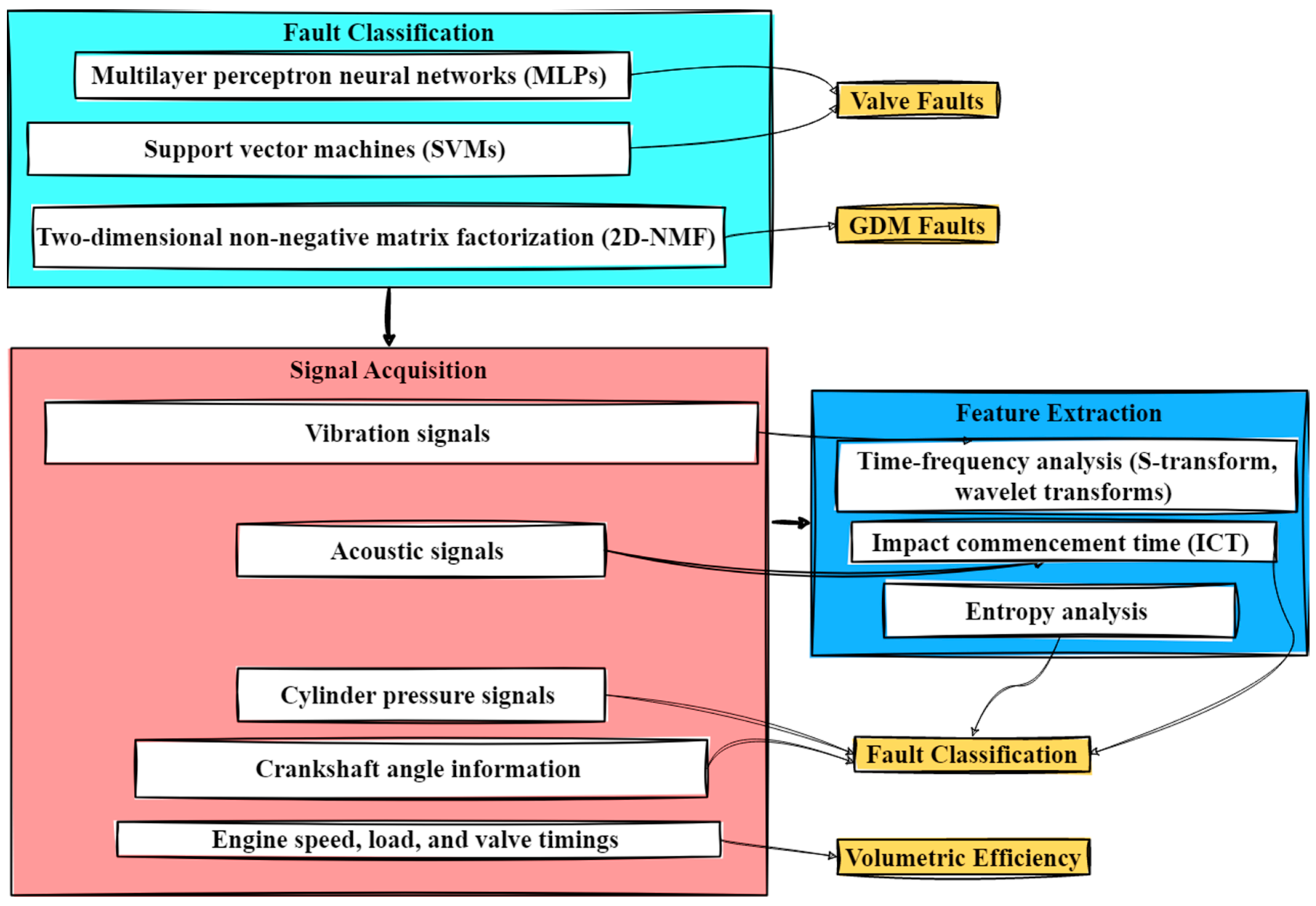
2.3. Valve
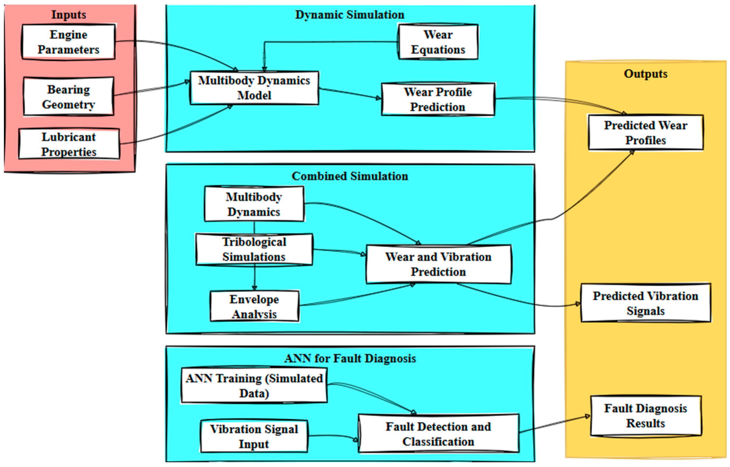
2.4. Bearing
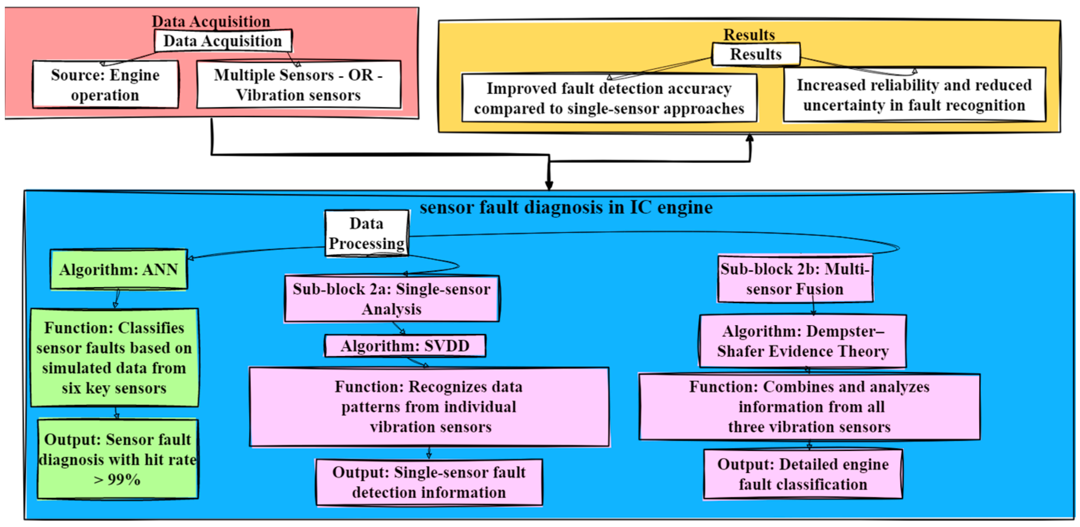
2.5. Sensor
2.6. Ignition
2.7. Injection
2.8. Hybrid
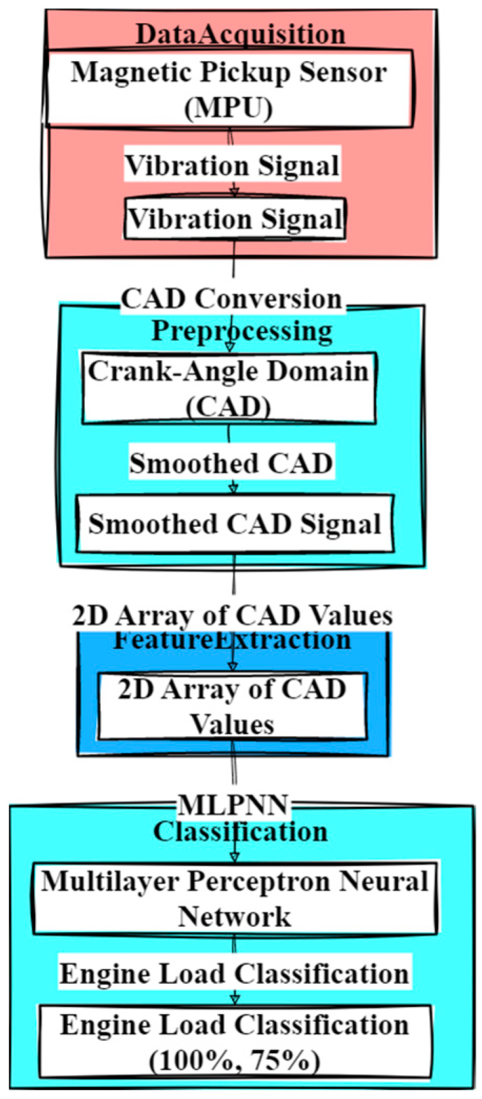
2.9. Engine Load
2.10. Others
2.11. Combustion
2.12. Deep Learning Approaches in Fault Diagnosis
Advanced Deep Learning Technique
3. Experimental Investigations
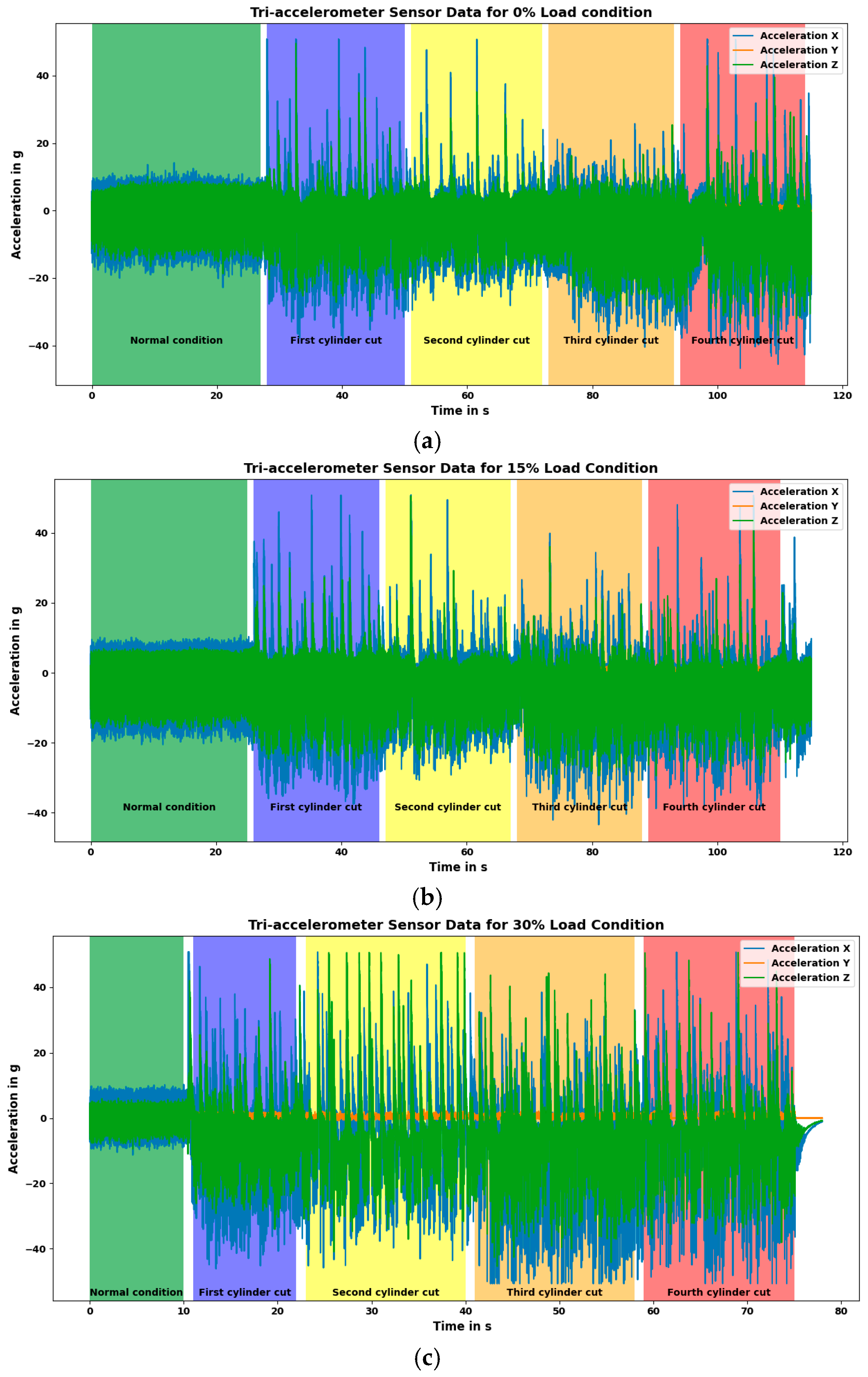
3.1. Experimental Setup
3.2. Methodology
3.3. Sensor Signal Graph
3.4. Classifiers Details
3.4.1. Decision Tree Classifier
3.4.2. Discriminant Classifiers
- (x)—input vector
- ()—covariance matrix
- —mean vector of class (k)
- —prior probability of class (k).
3.4.3. Naive Bayes Classifier
- P(y|x)—posterior probability of class (target) given predictor (attribute)
- P(y)—prior probability of class
- P(x|y)—likelihood which is the probability of predictor given class
- P(x)—prior probability of predictor.
- P(y|x)—posterior probability of class (target) given predictor (attribute)
- P(y)—prior probability of class
- P(x|y)—likelihood which is the probability of predictor given class
- P(x)—prior probability of predictor.
- K—kernel function (e.g., Gaussian, Epanechnikov, etc.)
- h—bandwidth
- m—number of observations.
3.4.4. Support Vector Machine (SVM) Classifiers
- w—weight vector to minimize
- X—data to classify
- b—bias term, or the linear coefficient estimated from the training data.
- X1 and X2 are the data points
- γ—parameter that defines how far the influence of a single training example reaches.
3.4.5. K-Nearest Neighbors (KNN) Classifier
- x and y are two points in the n-dimensional space
- xi and yi are the coordinates of points x and y, respectively.
- C—centroid
- n—number of points in the cluster
- xi—coordinate of the i-th point in the cluster.
3.4.6. Ensemble Machine Learning Classifier
- —predicted output
- K—number of trees
- wi—weight of the i-th tree
- fi(x) is the prediction of the i-th tree.
- —predicted output
- B is the number of trees
- Tb(x) is the prediction of the b-th tree.
3.4.7. Neural Network Classifiers
- Input Layer: the input layer passes the input data to the next layer without any transformation.
- Hidden Layers: for each neuron j in the hidden layer,
- zj is the weighted sum of inputs plus bias for neuron j
- Xi is the input from the previous layer
- Wij is the weight connecting neuron i in the previous layer to neuron j in the current layer
- bj is the bias for neuron j
- σ is the activation function
- aj is the output (activation) of neuron j.
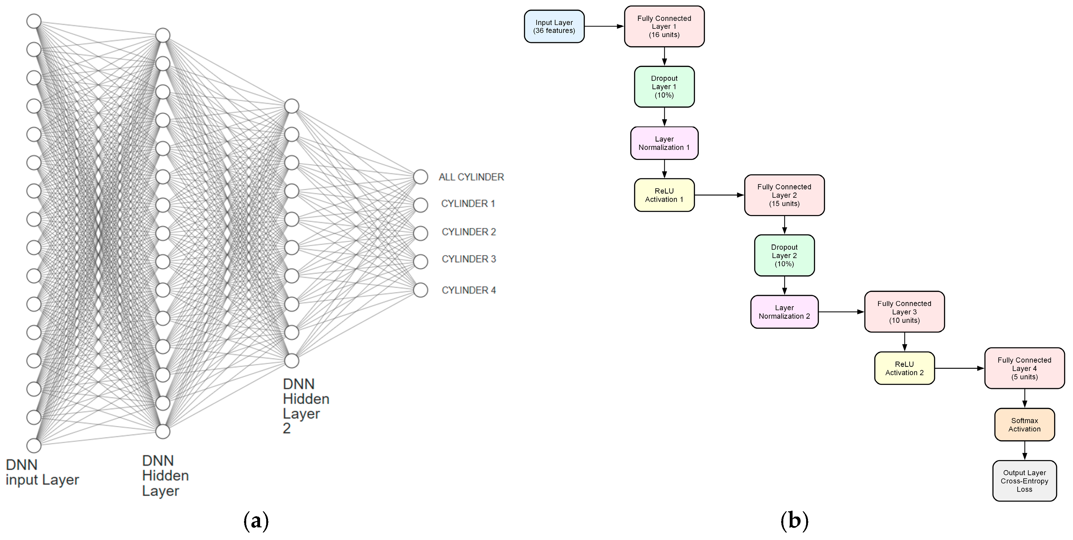
Proposed DNN Architecture
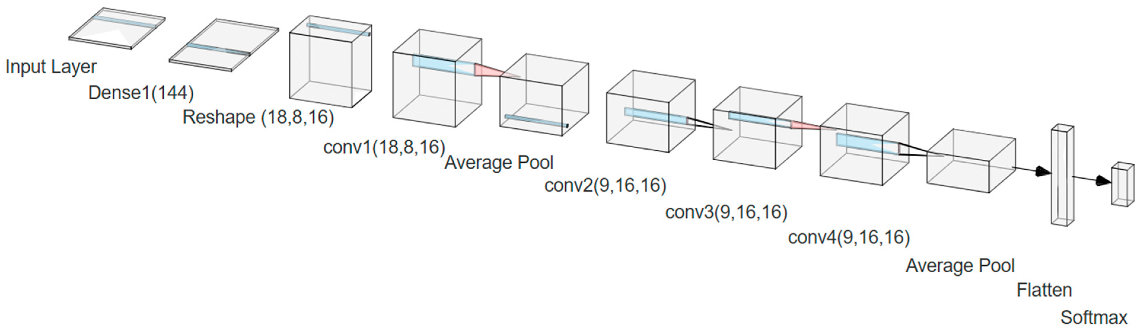
Proposed 1D-CNN Architecture
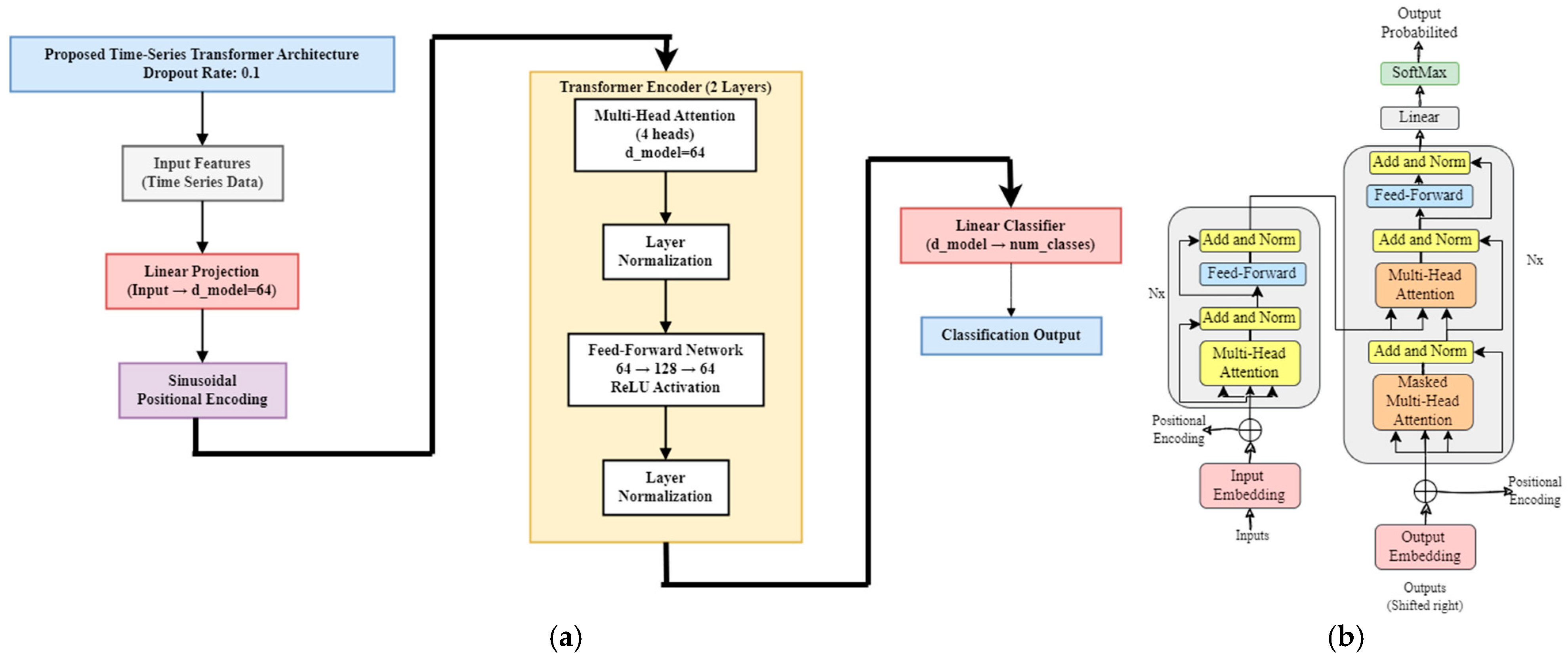
Proposed Transformer Architecture
Positional Encoding
Self-Attention
- The input matrix is element-wise multiplied by trainable matrices Wq, Wk, and Wv to form the Query, Key, and Value matrices.
- Upon this, a dot product and SoftMax are performed, followed by element-wise multiplication with the Value matrix, comprising the attention weights.
- Q—Query matrix
- Wq—Trainable weight matrix for query
- K—Key matrix
- Wk—trainable weight matrix for key
- V—Value matrix
- Wv—trainable weight matrix for value
- D—dmodel, number for model size
- Y—computed attention matrix.
Multi-Headed Attention Mechanism
Encoder Layer
Decoder Layer
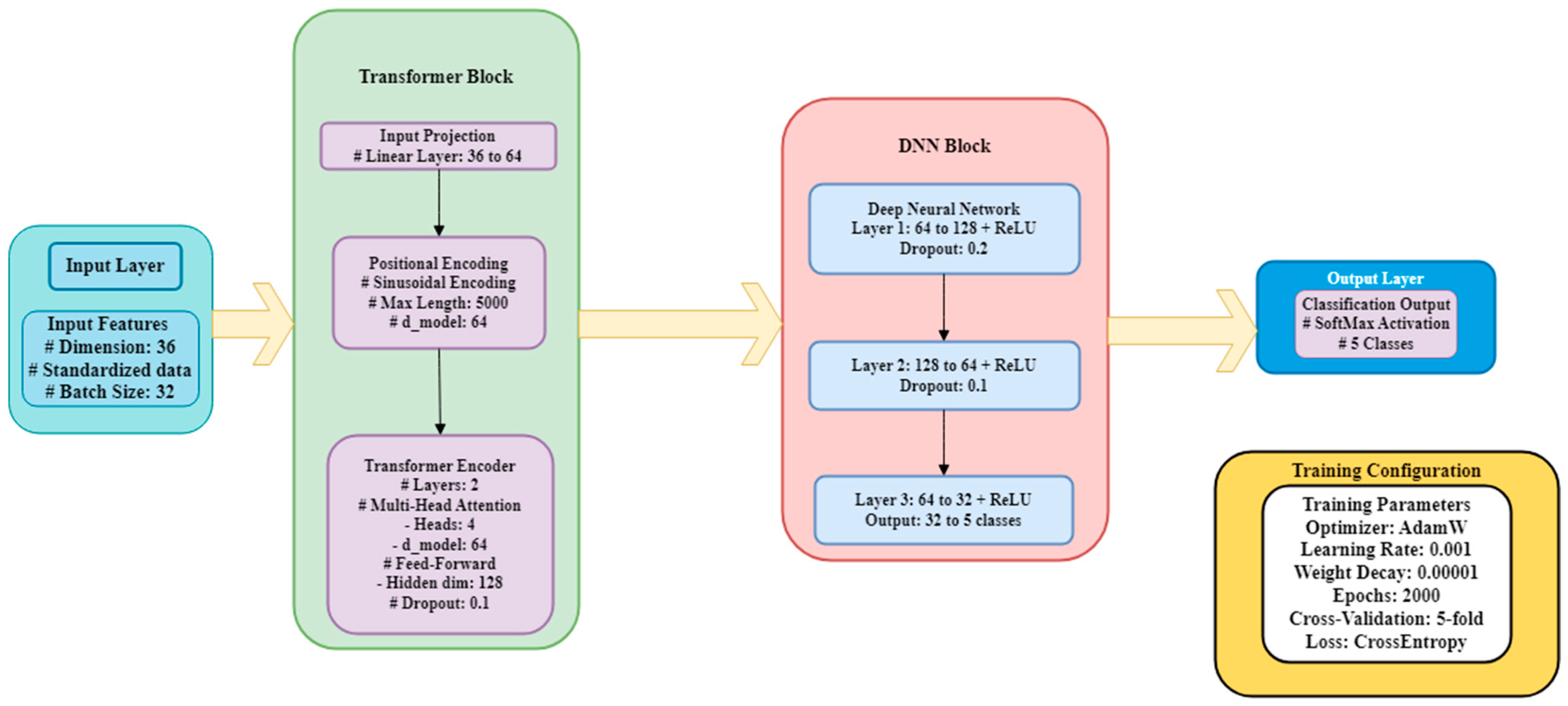
Proposed Hybrid Model Combining Transformers and Deep Neural Networks (DNNs) Architecture for Engine Fault Diagnosis
3.5. Importance of Data Transformation and Feature Selection
3.5.1. Feature Ranking
Chi2
- Σ = sum over all categories of the feature
- O = observed frequency of a particular outcome (e.g., cylinder cutoff) for a specific category
- E = expected frequency of the same outcome, calculated based on the null hypothesis that the feature and target variable are independent.
ANOVA
- Between-group variance (SSB): measures the variability between the means of different groups (cylinder states).
- Within-group variance (SSE): measures the variability within each group.
ReliefF Iterates Through Data Points
- Calculate the difference in the feature value between the data point and each NH (diff_hitj).
- Calculate the difference in the feature value between the data point and each NM (diff_missj).
- m = number of features
- k = number of nearest neighbors.
MRMR Utilizes Two Measures to Select Features
- F—Feature
- C—Target variable
- Fi—other selected features
- m—number of features.
- Fi—other selected features
- S—number of already selected features.
Kruskal–Wallis’s Test
- H—Kruskal–Wallis statistic
- N—total number of samples
- nj—number of samples in group j (e.g., running cylinder)
- Rj—sum of ranks in group j
- K—number of groups (cylinder states).
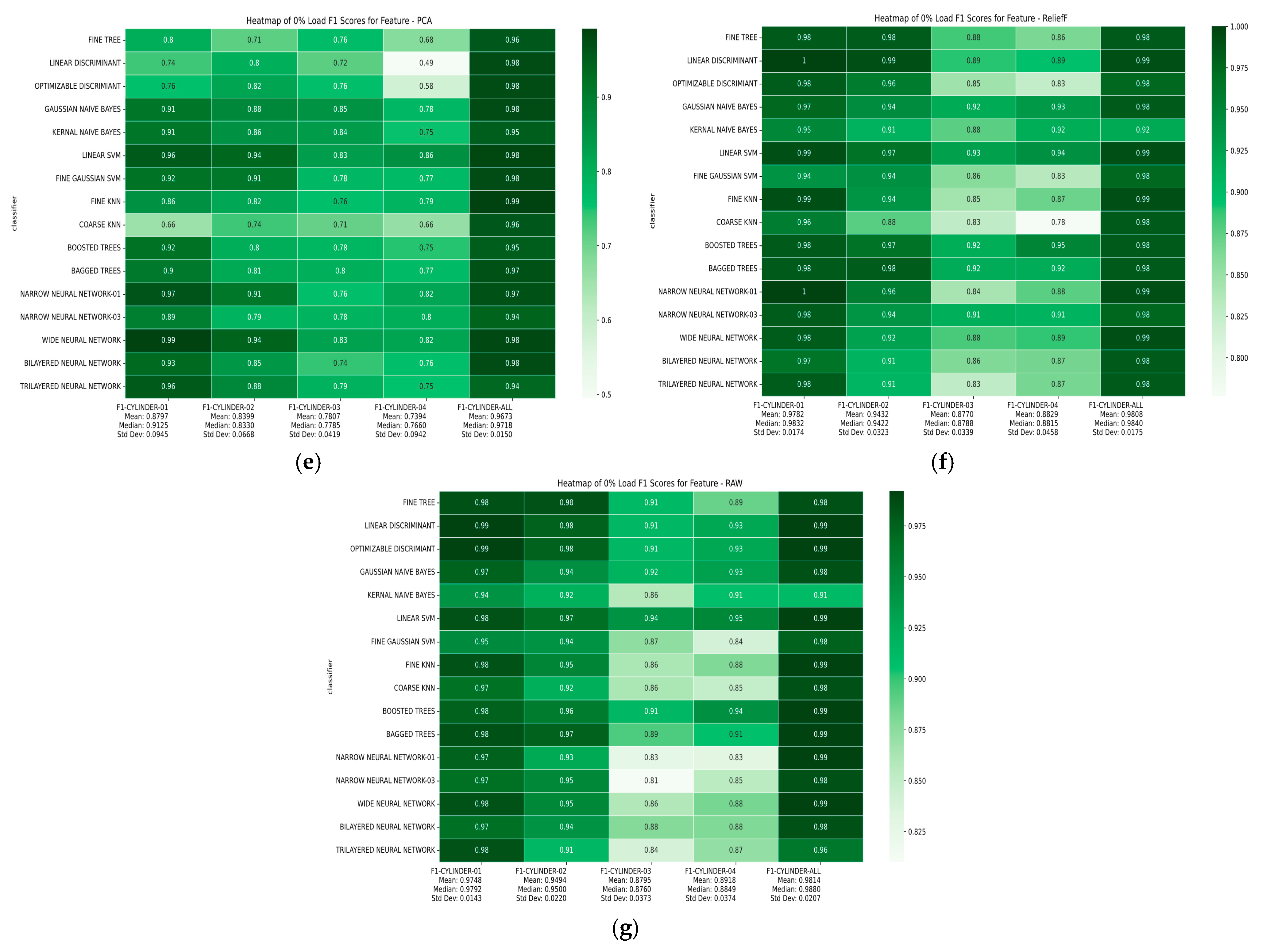
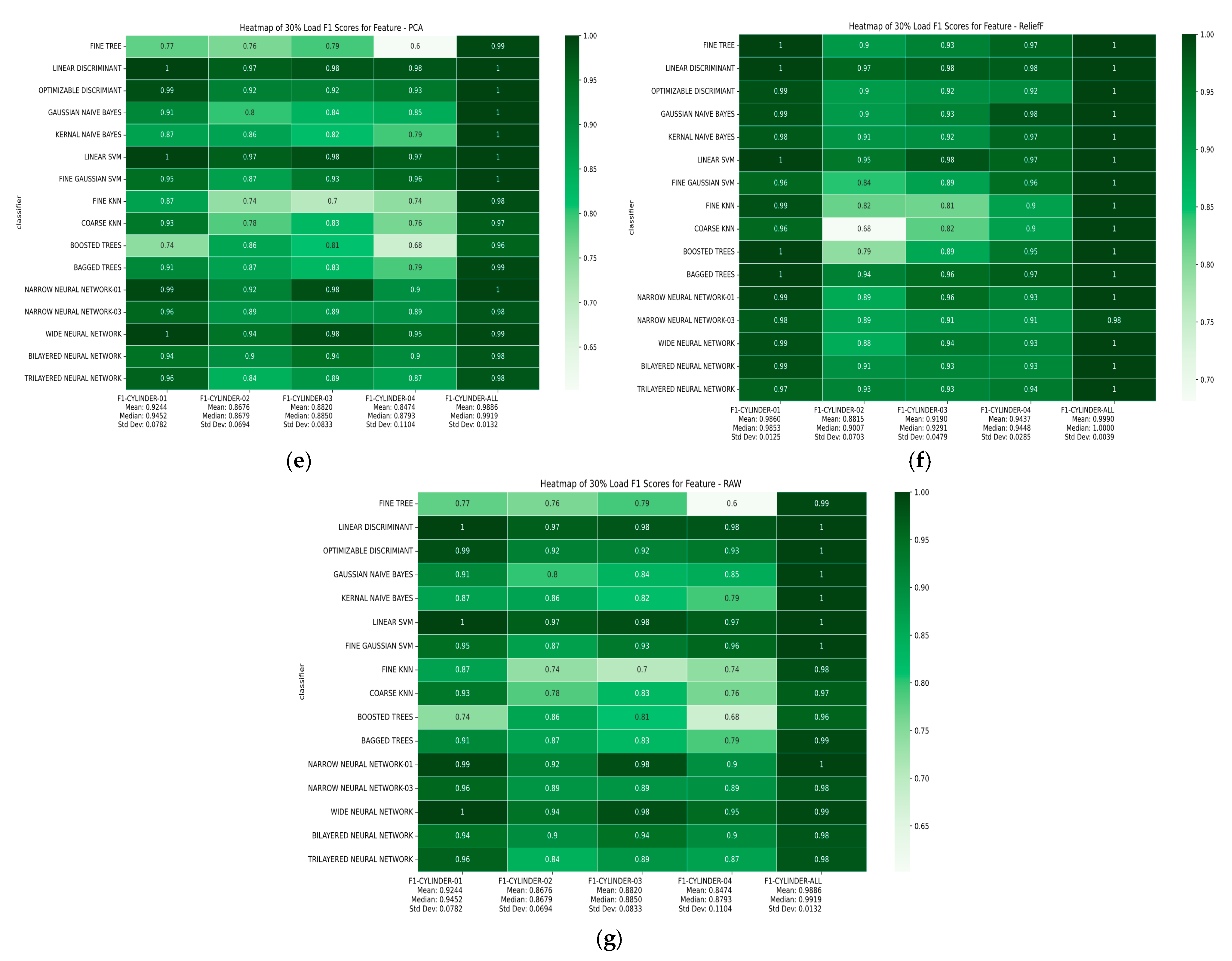
4. Result Metrics Calculation and Discussion
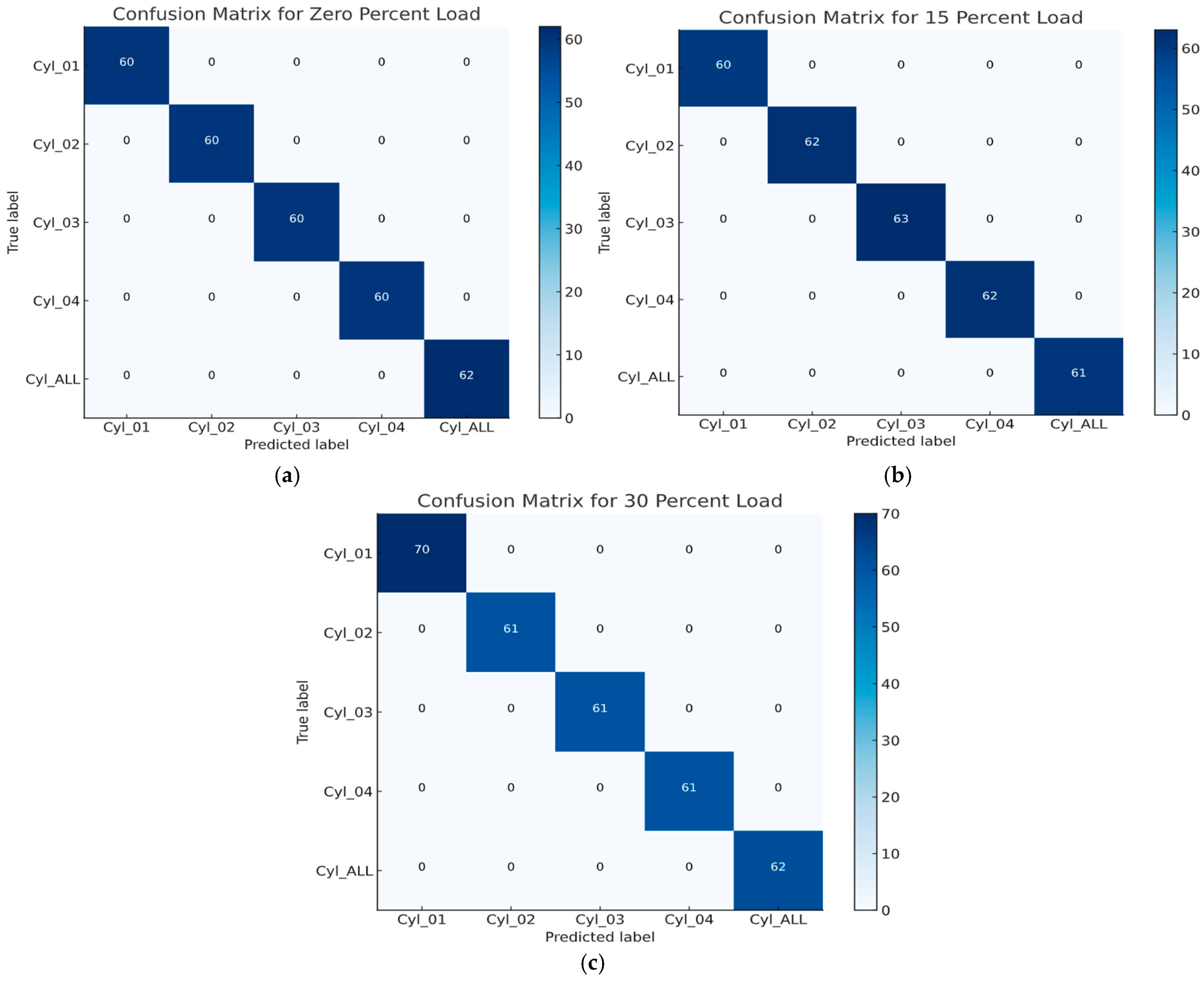
4.1. Confusion Matrix
- The rows represent the actual classes or labels.
- The columns represent the predicted classes made by the model.
4.1.1. Accuracy
- TP (True Positives): correctly predicted positive cases.
- TN (True Negatives): correctly predicted negative cases.
- FP (False Positives): incorrectly predicted positive cases (Type I error).
- FN (False Negatives): incorrectly predicted negative cases (Type II error).
4.1.2. Total Cost
4.1.3. F1 Score
- Precision: proportion of true positives among all predicted positives (TP/(TP + FP))
- Recall: proportion of actual positives that are correctly identified (TP/(TP + FN))
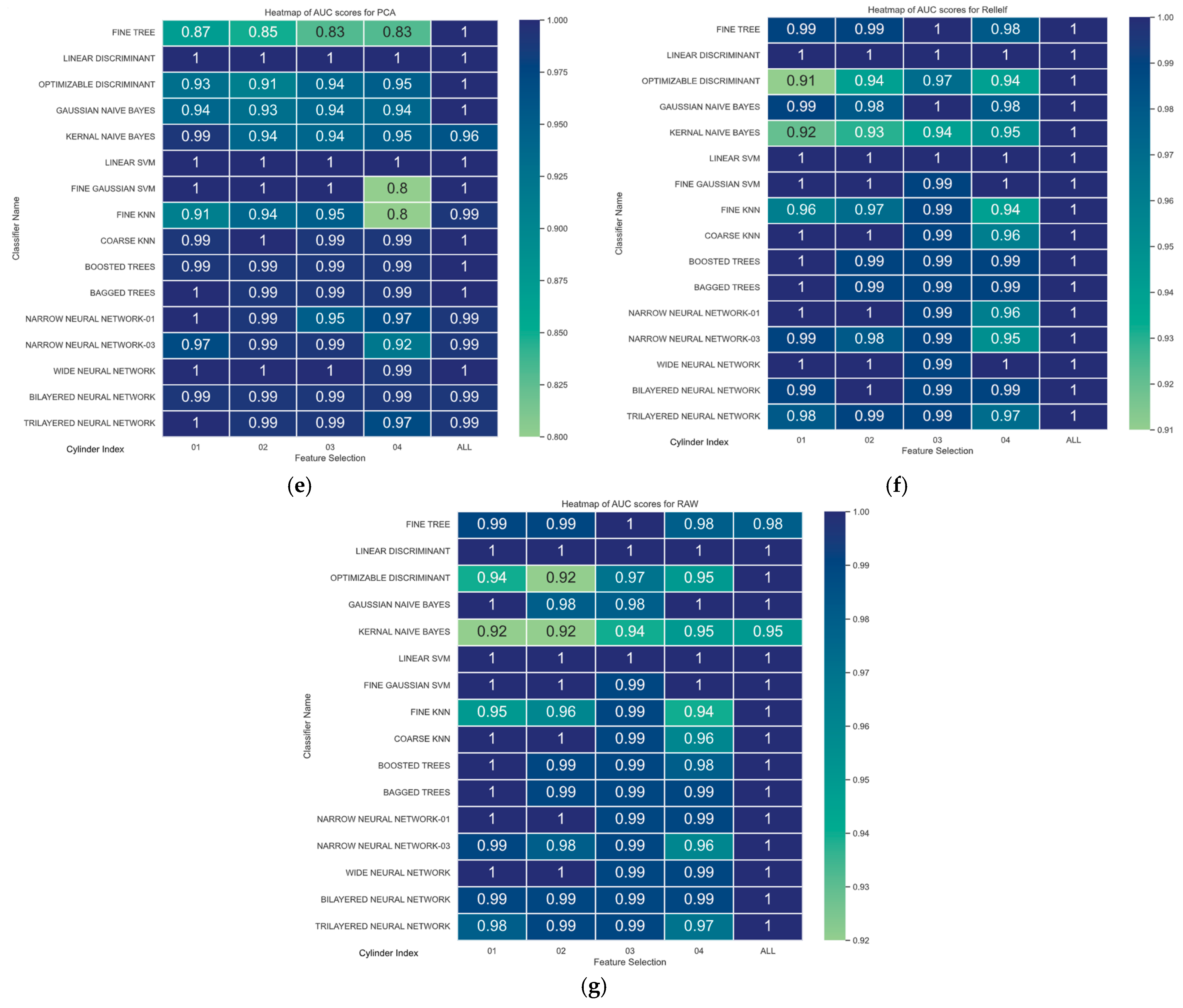
4.1.4. RoC Curve
0% Load Condition ROC Curve AuC Study
15% Load Condition RoC Curve AuC Study
30% Load Condition RoC Curve AuC Study
4.2. Deep Learning Approach Result Discussion
4.2.1. Proposed DNN Architecture Performance Evaluation
4.2.2. Proposed 1D-CNN Architecture Performance Evaluation
4.2.3. Proposed Transformer Architecture Performance Evaluation
4.2.4. Proposed Hybrid—Transformer and DNN Architecture Performance Evaluation
5. Future Scope
6. Conclusions
Author Contributions
Funding
Institutional Review Board Statement
Informed Consent Statement
Data Availability Statement
Conflicts of Interest
Abbreviations
| ICEs | Internal Combustion Engines |
| PCA | Principal Component Analysis |
| ANNs | Artificial Neural Networks |
| MAF | Manifold Air Fuel |
| MTMR | Modified Triple Modular Redundancy |
| PI | Proportional-Integral (controller) |
| EGT | Exhaust Gas Temperature |
| GA | Genetic Algorithm |
| MAP | Manifold Absolute Pressure |
| HFTC | Hybrid Fault-Tolerant Control System |
| AFTCS | Active Fault-Tolerant Control System |
| PFTCS | Passive Fault-Tolerant Control System |
| CWT | Continuous Wavelet Transform |
| STFT | Short-Time Fourier Transform |
| FFT | Fast Fourier Transform |
| SVM | Support Vector Machine |
| NN | Neural Network |
| GDM | Gas Distribution Mechanism |
| CNN | Convolutional Neural Network |
| ARMA | Autoregressive Moving Average |
| XGBoost | Extreme Gradient Boosting |
| VMD | Variational Mode Decomposition |
| GWO | Grey Wolf Optimization |
| SVDD | Support Vector Data Description |
| GRNN | General Regression Neural Network |
| TFR | Time-Frequency Representation |
| ICA | Independent Component Analysis |
| FCM | Fuzzy C-Means |
| EMD | Empirical Mode Decomposition |
| ITD | Intrinsic Time-Scale Decomposition |
| DSM | Damped Sinusoid Model |
| MLPNN | Multilayer Perceptron Neural Network |
| CAD | Crank-Angle Degree |
| CCV | Combustion Cycle Variability |
| MRMR | Minimum Redundancy Maximum Relevance |
| Chi2 | Chi-Square Test |
| ReliefF | Relief Feature Selection Algorithm |
| ANOVA | Analysis of Variance |
| ROC-AUC | Receiver Operating Characteristic—Area Under the Curve |
| BP | Backpropagation |
| MFCC | Mel-Frequency Cepstral Coefficients |
| DTW | Dynamic Time Warping |
| EEMD | Ensemble Empirical Mode Decomposition |
| WPT | Wavelet Packet Transform |
| WVD | Wigner-Ville Distribution |
| HHT | Hilbert-Huang Transform |
| LIASSR | Least Instantaneous Angular Speed Reduction |
| AFR | Air–Fuel Ratio |
| DAQ | Data Acquisition |
| MAD | Mean Absolute Deviation |
| IQR | Interquartile Range |
| KNN | K-Nearest Neighbors |
| ROC | Receiver Operating Characteristic |
| PPV | Positive Predictive Value |
| FDR | False Discovery Rate |
| TPR | True Positive Rate |
| FNR | False Negative Rate |
| LDA | Linear Discriminant Analysis |
| KDE | Kernel Density Estimation |
| GNB | Gaussian Naive Bayes |
| SSB | Between-group Sum of Squares |
| SSE | Within-group Sum of Squares |
| NH | Nearest Hits |
| NM | Nearest Misses |
| TP | True Positives |
| TN | True Negatives |
| FP | False Positives |
| FN | False Negative |
| RAW | “Unprocessed |
| FPR | false positive rate |
| TNR | true negative rate |
| AuC | Area under the Curve |
Appendix A


References
- Gao, Z.; Cecati, C.; Ding, S.X. A Survey of Fault Diagnosis and Fault-Tolerant Techniques—Part I: Fault Diagnosis with Model-Based and Signal-Based Approaches. IEEE Trans. Ind. Electron. 2015, 62, 3757–3767. [Google Scholar] [CrossRef]
- Gao, Z.; Cecati, C.; Ding, S.X. A Survey of Fault Diagnosis and Fault-Tolerant Techniques—Part II: Fault Diagnosis with Knowledge-Based and Hybrid/Active Approaches. IEEE Trans. Ind. Electron. 2015, 62, 3768–3774. [Google Scholar] [CrossRef]
- Iqbal, M.S.; Amin, A.A. Genetic algorithm based active fault-tolerant control system for air fuel ratio control of internal combustion engines. Meas. Control. 2022, 55, 703–716. [Google Scholar] [CrossRef]
- Sakthivel, N.R.; Sugumaran, V.; Nair, B.B. Application of Support Vector Machine (SVM) and Proximal Support Vector Machine (PSVM) for fault classification of monoblock centrifugal pump. Int. J. Data Anal. Tech. Strateg. 2010, 2, 38–61. [Google Scholar] [CrossRef]
- Haneef, M.D.; Randall, R.B.; Smith, W.A.; Peng, Z. Vibration and Wear Prediction Analysis of IC Engine Bearings by Numerical Simulation. Wear 2017, 384, 15–27. [Google Scholar] [CrossRef]
- León, P.G.; García-Morales, J.; Escobar-Jiménez, R.; Gómez-Aguilar, J.; López-López, G.; Torres, L. Implementation of a fault tolerant system for the internal combustion engine’s MAF sensor. Measurement 2018, 122, 91–99. [Google Scholar] [CrossRef]
- Roy, S.K.; Mohanty, A.R.; Kumar, C.S. In-cylinder combustion detection based on logarithmic instantaneous angular successive speed ratio. J. Phys. Conf. Ser. 2019, 1240, 012037. [Google Scholar] [CrossRef]
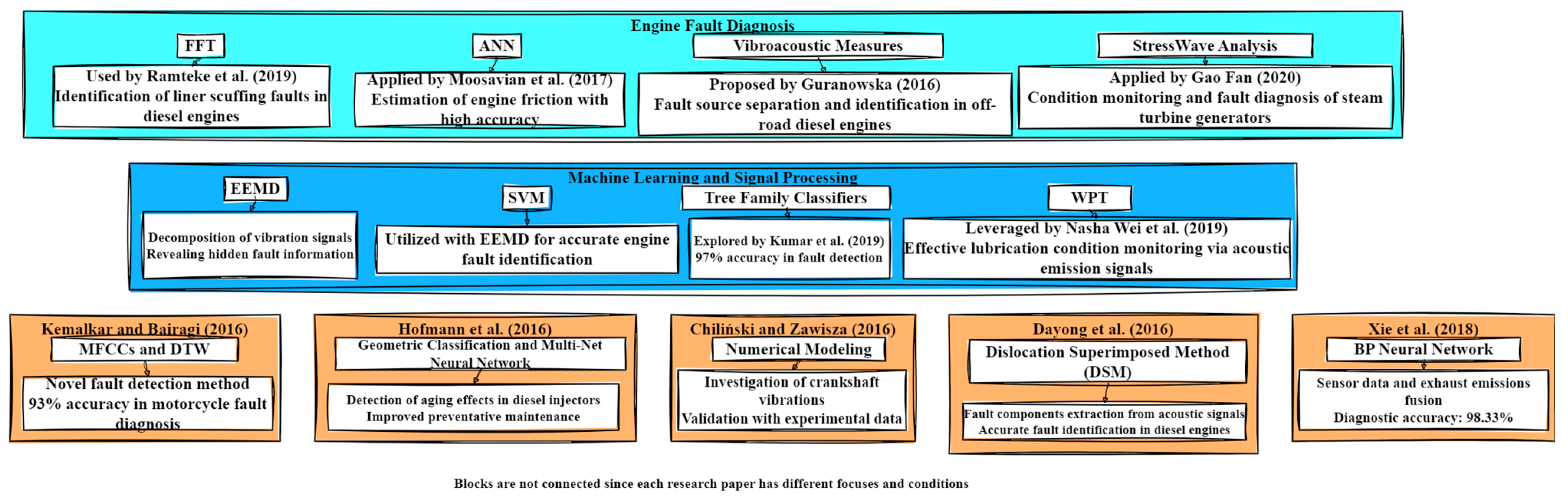
- Moosavian, A.; Najafi, G.; Ghobadian, B.; Mirsalim, M.; Jafari, S.M.; Sharghi, P. Piston scuffing fault and its identification in an IC engine by vibration analysis. Appl. Acoust. 2016, 103, 108–120. [Google Scholar] [CrossRef]
- Zhang, Y.; Yang, Y.; Li, H.; Han, H.; He, Z. Layer-Wise Fault Diagnosis Based on Key Performance Indicator for Cylinder-Piston Assembly of Diesel Engine. In Proceedings of the IEEE 15th International Conference on Control and Automation (ICCA), Edinburgh, UK, 16–19 July 2019; pp. 307–312. [Google Scholar]
- Jafarian, K.; Mobin, M.; Jafari-Marandi, R.; Rabiei, E. Misfire and valve clearance faults detection in the combustion engines based on a multi-sensor vibration signal monitoring. Measurement 2018, 128, 527–536. [Google Scholar]
- Stojanovic, S.; Tebbs, A.; Samuel, S.; Durodola, J. Cepstrum Analysis of a Rate Tube Injection Measurement Device; SAE Technical Paper 2016-01-2196; SAE International: Detroit, MI, USA, 2016. [Google Scholar]
- Cao, W.; Dong, G.; Xie, Y.-B.; Peng, Z. Prediction of wear trend of engines via on-line wear debris monitoring. Tribol. Int. 2018, 120, 510–519. [Google Scholar] [CrossRef]
- Kumar, A.; Gupta, R.; Singh, P. Hybrid methods for misfire detection using threshold-based algorithm on WVD and HHT with Android mobile sound recording. J. Combust. Emiss. 2023, 19, 302–314. [Google Scholar]
- Ftoutou, E.; Chouchane, M. Feature Extraction Using S-Transform and 2DNMF for Diesel Engine Faults Classification. In Applied Condition Monitoring, Proceedings of the International Conference on Acoustics and Vibration (ICAV2016), Hammamet, Tunisia, 21–23 March 2016; Fakhfakh, T., Chaari, F., Walha, L., Abdennadher, M., Abbes, M., Haddar, M., Eds.; Springer: Berlin/Heidelberg, Germany, 2017; Volume 5. [Google Scholar]
- Moosavian, A.; Najafi, G.; Ghobadian, B.; Mirsalim, M. The effect of piston scratching fault on the vibration behavior of an IC engine. Appl. Acoust. 2017, 126, 91–100. [Google Scholar] [CrossRef]
- McMahan, J.B. Functional Principal Component Analysis of Vibrational Signal Data: A Functional Data Analytics Approach for Fault Detection and Diagnosis of Internal Combustion Engines. Ph.D. Thesis, Mississippi State University, Starkville, MI, USA, 2018. [Google Scholar]
- Hofmann, O.; Strauß, P.; Schuckert, S.; Huber, B.; Rixen, D.; Wachtmeister, G. Identification of Aging Effects in Common Rail Diesel Injectors Using Geometric Classifiers and Neural Networks; SAE Technical Paper 2016-01-0813; SAE International: Detroit, MI, USA, 2016. [Google Scholar]
- Zheng, T.; Tan, R.; Li, Y.; Yang, B.; Shi, L.; Zhou, T. Fault diagnosis of internal combustion engine valve clearance: The survey of the-state-of-the-art. In Proceedings of the 12th World Congress on Intelligent Control and Automation (WCICA), Guilin, China, 12–15 June 2016; pp. 2614–2619. [Google Scholar]
- Zhao, C.; Shen, W. A Federated Distillation Domain Generalization Framework for Machinery Fault Diagnosis with Data Privacy. Eng. Appl. Artif. Intell. 2024, 130, 107765. [Google Scholar] [CrossRef]
- Khoualdia, T.; Lakehal, A.; Chelli, Z. Practical investigation on bearing fault diagnosis using massive vibration data and artificial neural network. In Big Data and Networks Technologies; Springer: Berlin/Heidelberg, Germany, 2019; pp. 110–116. [Google Scholar]
- Jiang, Z.; Mao, Z.; Wang, Z.; Zhang, J. Fault Diagnosis of Internal Combustion Engine Valve Clearance Using the Impact Commencement Detection Method. Sensors 2017, 17, 2916. [Google Scholar] [CrossRef] [PubMed]
- Moosavian, A.; Ahmadi, H.; Sakhaei, B.; Labbafi, R. Support vector machine and K-nearest neighbour for unbalanced fault detection. J. Qual. Maint. Eng. 2014, 20, 65–75. [Google Scholar] [CrossRef]
- Kemalkar, A.K.; Bairagi, V.K. Engine fault diagnosis using sound analysis. In Proceedings of the 2016 International Conference on Automatic Control and Dynamic Optimization Techniques (ICACDOT), Pune, India, 9–10 September 2016; pp. 943–946. [Google Scholar]
- Gritsenko, A.; Shepelev, V.; Zadorozhnaya, E.; Almetova, Z.; Burzev, A. The advancement of the methods of vibro-acoustic control of the ICE gas distribution mechanism. FME Trans. 2020, 48, 127–136. [Google Scholar] [CrossRef]
- Ates, C.; Höfchen, T.; Witt, M.; Koch, R.; Bauer, H.J. Vibration-based wear condition estimation of journal bearings using convolutional autoencoders. Sensors 2023, 23, 9212. [Google Scholar] [CrossRef] [PubMed]
- Figlus, T.; Gnap, J.; Skrúcaný, T.; Šarkan, B.; Stoklosa, J. The Use of Denoising and Analysis of Acoustic Signal Entropy in Diagnosing Engine Valve Clearance. Entropy 2016, 18, 253. [Google Scholar] [CrossRef]
- Zabihi-Hesari, A.; Ansari-Rad, S.; Shirazi, F.A.; Ayati, M. Fault detection and diagnosis of a 12-cylinder trainset diesel engine based on vibration signature analysis and neural network. Proc. Inst. Mech. Eng. Part C J. Mech. Eng. Sci. 2019, 233, 1910–1923. [Google Scholar] [CrossRef]
- Wang, A.; Li, Y.; Du, X.; Zhong, C. Diesel Engine Gearbox Fault Diagnosis Based on Multi-features Extracted from Vibration Signals. IFAC-Pap. 2021, 54, 33–38. [Google Scholar] [CrossRef]
- Mulay, S.; Sugumaran, V.; Devasenapati, S.B. Misfire detection in I.C. engine through ARMA features using machine learning approach. Prog. Ind. Ecol. Int. J. 2018, 12, 93–111. [Google Scholar]
- Rameshkumar, K.; Natarajan, K.; Krishnakumar, P.; Saimurugan, M. Machine Learning Approach for Predicting the Solid Particle Lubricant Contamination in a Spherical Roller Bearing. IEEE Access 2024, 12, 78680–78700. [Google Scholar] [CrossRef]
- Ghajar, M.; Kakaee, A.H.; Mashadi, B. Semi-empirical modeling of volumetric efficiency in engines equipped with variable valve timing system. J. Cent. South Univ. 2016, 23, 3132–3142. [Google Scholar] [CrossRef]
- Firmino, R.; da Silva, F.G.; dos Santos, A.C. A comparative study of acoustic and vibration signals for bearing fault detection and diagnosis based on MSB analysis. Measurement 2020, 154, 107465. [Google Scholar]
- Kumar, N.; Sakthivel, G.; Jegadeeshwaran, R.; Sivakumar, R.; Kumar, S. Vibration Based IC Engine Fault Diagnosis Using Tree Family Classifiers—A Machine Learning Approach. In Proceedings of the 2019 IEEE International Symposium on Smart Electronic Systems (iSES) (Formerly iNiS), Rourkela, India, 16–18 December 2019; pp. 225–228. [Google Scholar]
- Ferrari, A.; Paolicelli, F. A virtual injection sensor by means of time frequency analysis. Mech. Syst. Signal Process. 2019, 116, 832–842. [Google Scholar] [CrossRef]
- Komorska, I.; Wołczyński, Z.; Borczuch, A. Diagnosis of sensor faults in a combustion engine control system with the artificial neural network. Diagnostyka 2019, 20, 19–25. [Google Scholar] [CrossRef]
- Zhou, Y.; Wang, Z.; Zuo, X.; Zhao, H. Identification of wear mechanisms of main bearings of marine diesel engine using recurrence plot based on CNN model. Wear 2023, 520, 204656. [Google Scholar] [CrossRef]
- Mu, J.; Liu, X.; Chen, Y.; Zhang, H. Fault diagnosis using MICEEMD-PWVD and TD-2DPCA for valve clearance in combustion engines. J. Sound Vib. 2021, 500, 116003. [Google Scholar]
- Sumanth, M.N.; Murugesan, S. Experimental Investigation of Wall Wetting Effect on Hydrocarbon Emission in Internal Combustion Engine. IOP Conf. Ser. Mater. Sci. Eng. 2019, 577, 012029. [Google Scholar] [CrossRef]
- Vichi, G.; Becciani, M.; Stiaccini, I.; Ferrara, G.; Ferrari, L.; Bellissima, A.; Asai, G. Analysis of the Turbocharger Speed to Estimate the Cylinder-to-Cylinder Injection Variations-Part 2-Frequency Domain Analysis; SAE Technical Paper 2016-32-0085; SAE International: Detroit, MI, USA, 2016. [Google Scholar]
- Kang, J.; Zhang, X.; Zhang, D.; Liu, Y. A Condition-Monitoring Approach for Diesel Engines Based on an Adaptive VMD and Sparse Representation Theory. Energies 2022, 15, 3315. [Google Scholar] [CrossRef]
- Tao, J.; Qin, C.; Li, W.; Liu, C. Intelligent Fault Diagnosis of Diesel Engines via Extreme Gradient Boosting and High-Accuracy Time–Frequency Information of Vibration Signals. Sensors 2019, 19, 3280. [Google Scholar] [CrossRef] [PubMed]
- Yang, X.; Bi, F.; Cheng, J.; Tang, D.; Shen, P.; Bi, X. A Multiple Attention Convolutional Neural Networks for Diesel Engine Fault Diagnosis. Sensors 2024, 24, 2708. [Google Scholar] [CrossRef] [PubMed]
- Becciani, M.; Romani, L.; Vichi, G.; Bianchini, A.; Asai, G.; Minamino, R.; Bellissima, A.; Ferrara, G. Innovative Control Strategies for the Diagnosis of Injector Performance in an Internal Combustion Engine via Turbocharger Speed. Energies 2019, 12, 1420. [Google Scholar] [CrossRef]
- Shahid, S.M.; Ko, S.; Kwon, S. Real-time abnormality detection and classification in diesel engine operations with convolutional neural network. Expert Syst. Appl. 2022, 192, 116233. [Google Scholar]
- Radhika, N.; Sabarinathan, M.; Jen, T.-C. Machine learning based prediction of Young’s modulus of stainless steel coated with high entropy alloys. Results Mater. 2024, 23, 100607. [Google Scholar] [CrossRef]
- Merkisz-Guranowska, A.; Waligórski, M. Recognition and Separation Technique of Fault Sources in Off-Road Diesel Engine Based on vibroacoustic Signal. J. Vib. Eng. Technol. 2018, 6, 263–271. [Google Scholar] [CrossRef]
- Chen, L.; Zhang, Y.; Wang, M.; Li, P.; Liu, Q. Statistical pattern recognition using DSM (Dislocation Superimposed Method) for fault isolation: Extracting impulsive fault components from acoustic signals in gasoline engines. Hybrid J. Engine Fault Anal. 2013. [Google Scholar]
- Shan, C.; Chin, C.S.; Mohan, V.; Zhang, C. Review of various machine learning approaches for predicting parameters of lithium-ion batteries in electric vehicles. Batteries 2024, 10, 181. [Google Scholar] [CrossRef]
- Zhang, K.; Wu, J.; Li, S.; Chen, Y.; Zhao, X. Hybrid methods using EMD-SVM for fault diagnosis: Combining signal decomposition with machine learning for rolling bearing fault diagnosis. J. Roll. Bear. Fault Diagn. 2022. [Google Scholar]
- Xie, C.; Wang, Y.; MacIntyre, J.; Sheikh, M.; Elkady, M. Using Sensors Data and Emissions Information to Diagnose Engine’s Faults. Int. J. Comput. Intell. Syst. 2018, 11, 1142–1152. [Google Scholar] [CrossRef]
- Ftoutou, E.; Chouchane, M. Diesel Engine Injection Faults’ Detection and Classification Utilizing Unsupervised Fuzzy Clustering Techniques. Proc. Inst. Mech. Eng. Part C J. Mech. Eng. Sci. 2019, 233, 5622–5636. [Google Scholar] [CrossRef]
- Kannan, N.; Saimurugan, M.; Sowmya, S.; Edinbarough, I. Enhanced quadratic discriminant analysis with sensor signal fusion for speed-independent fault detection in rotating machines. Engine IOP Conf. Ser. Meas. Sci. Technol. 2013, 34, 12. [Google Scholar]
- Waligórski, M.; Batura, K.; Kucal, K.; Merkisz, J. Empirical assessment of thermodynamic processes of a turbojet engine in the process values field using vibration parameters. Measurement 2020, 158, 107702. [Google Scholar] [CrossRef]
- Saimurugan, M.; Ramachandran, K.I.; Sugumaran, V.; Sakthivel, N.R. Multi component fault diagnosis of rotational mechanical system based on decision tree and support vector machine. Expert Syst. Appl. 2011, 38, 3819–3826. [Google Scholar] [CrossRef]
- Li, N. Determination of knock characteristics in spark ignition engines: An approach based on ensemble empirical mode decomposition Meas. Sci. Technol. 2016, 27, 045109. [Google Scholar] [CrossRef]
- Yao, X.; Wang, L.; Chen, M.; Li, J.; Zhang, Q. Hybrid methods using Gammatone filter bank and Robust ICA for noise source identification: Separating and identifying noise sources in internal combustion engines. J. Intern. Combust. Engine Noise Anal. 2017. [Google Scholar]
- Merkisz-Guranowska, A.; Waligórski, M. Analysis of vibroacoustic estimators for a heavy-duty diesel engine used in sea transport in the aspect of diagnostics of its environmental impact. J. Vibroengineering 2016, 18, 1346–1357. [Google Scholar] [CrossRef]
- Taghizadeh-Alisaraei, A.; Mahdavian, A. Fault detection of injectors in diesel engines using vibration time-frequency analysis. Appl. Acoust. 2019, 143, 48–58. [Google Scholar] [CrossRef]
- Dayong, N.; Changle, S.; Yongjun, G.; Zengmeng, Z.; Jiaoyi, H. Extraction of fault component from abnormal sound in diesel engines using acoustic signals. Mech. Syst. Signal Process. 2016, 75, 544–555. [Google Scholar] [CrossRef]
- Lilo, M.A.; Latiff, L.A.; Abu, A.B.; Mashhadany, Y.I. Vibration fault detection and classification based on the FFT and fuzzy logic. ARPN J. Eng. Appl. Sci. 2016, 11, 4633–4637. [Google Scholar]
- Zhao, H.; Zhang, J.; Jiang, Z.; Wei, D.; Zhang, X.; Mao, Z. A New Fault Diagnosis Method for a Diesel Engine Based on an Optimized Vibration Mel Frequency under Multiple Operation Conditions. Sensors 2019, 19, 2590. [Google Scholar] [CrossRef] [PubMed]
- Xu, Y.; Huang, B.; Yun, Y.; Cattley, R.; Gu, F.; Ball, A.D. Model Based IAS Analysis for Fault Detection and Diagnosis of IC Engine Powertrains. Energies 2020, 13, 565. [Google Scholar] [CrossRef]
- Shahbaz, M.; Iqbal, J.; Mehmood, A.; Aslam, M. Model-based diagnosis using an ANN-based observer for fault-tolerant control of air-fuel ratio in internal combustion engines. J. Electr. Eng. Technol. 2021, 16, 287–299. [Google Scholar]
- Bi, X.; Cao, S.; Zhang, D. A Variety of Engine Faults Detection Based on Optimized Variational Mode Decomposition–Robust Independent Component Analysis and Fuzzy C-Mean Clustering. IEEE Access 2019, 7, 27756–27768. [Google Scholar] [CrossRef]
- Ramteke, S.M.; Chelladurai, H.; Amarnath, M. Diagnosis of Liner Scuffing Fault of a Diesel Engine via Vibration and Acoustic Emission Analysis. J. Vib. Eng. Technol. 2019, 8, 815–833. [Google Scholar] [CrossRef]
- Liu, R.; Chen, X.; Zhang, Y.; Hu, W.; Wang, J. Hybrid methods using WPD-SVM for effective fault identification: Integrating wavelet packet decomposition and support vector machines for induction motor fault diagnosis. J. Induction Mot. Fault Diagn. 2021. [Google Scholar]
- Xu, H.; Liu, F.; Wang, Z.; Ren, X.; Chen, J.; Li, Q.; Zhu, Z. A Detailed Numerical Study of NOx Kinetics in Counterflow Methane Diffusion Flames: Effects of Fuel-Side versus Oxidizer-Side Dilution. J. Combust. Vol. 2021, 2021, 6642734. [Google Scholar] [CrossRef]
- Amin, A.A.; Mahmood-Ul-Hasan, K. Advanced Fault Tolerant Air-Fuel Ratio Control of Internal Combustion Gas Engine for Sensor and Actuator Faults. IEEE Access 2019, 7, 17634–17643. [Google Scholar] [CrossRef]
- Amin, A.; Mahmood-ul-Hasan, K. Hybrid fault tolerant control for air–fuel ratio control of internal combustion gasoline engine using Kalman filters with advanced redundancy. Meas. Control. 2019, 52, 473–492. [Google Scholar] [CrossRef]
- Alsuwian, T.; Tayyeb, M.; Amin, A.A.; Qadir, M.B.; Almasabi, S.; Jalalah, M. Design of a hybrid fault-tolerant control system for air–fuel ratio control of internal combustion engines using genetic algorithm and higher-order sliding mode control. Energies 2022, 15, 56s66. [Google Scholar] [CrossRef]
- Chen, J.; Randall, R.B.; Peeters, B. Advanced diagnostic system for piston slap faults in IC engines, based on the non-stationary characteristics of the vibration signals. Mech. Syst. Signal Process. 2016, 75, 434–454. [Google Scholar] [CrossRef]
- Chen, J.; Randall, R.B. Intelligent diagnosis of bearing knock faults in internal combustion engines using vibration simulation. Mech. Mach. Theory 2016, 104, 161–176. [Google Scholar] [CrossRef]
- Zeng, R.; Zhang, L.; Mei, J.; Shen, H.; Zhao, H. Fault detection in an engine by fusing information from multivibration sensors. Int. J. Distrib. Sens. Netw. 2017, 13. [Google Scholar] [CrossRef]
- Kang, J.; Zhang, X.; Zhang, D.; Liu, Y. Pressure drops and mixture friction factor for gas–liquid two-phase transitional flows in a horizontal pipe at low gas flow rates. Chem. Eng. Sci. 2021, 246, 117011. [Google Scholar] [CrossRef]
- Awad, O.I.; Zhang, Z.; Kamil, M.; Ma, X.; Ali, O.M.; Shuai, S. Wavelet Analysis of the Effect of Injection Strategies on Cycle to Cycle Variation GDI Optical Engine under Clean and Fouled Injector. Processes 2019, 7, 817. [Google Scholar] [CrossRef]
- Wang, Y.; Zhang, F.; Cui, T.; Zhou, J. Fault diagnosis for manifold absolute pressure sensor (MAP) of diesel engine based on Elman neural network observer. Chin. J. Mech. Eng. 2016, 29, 386–395. [Google Scholar] [CrossRef]
- Ftoutou, E.; Chouchane, M. Injection Fault Detection of a Diesel Engine by Vibration Analysis. In Design and Modeling of Mechanical Systems—III. CMSM 2017; Lecture Notes in Mechanical Engineering; Haddar, M., Chaari, F., Benamara, A., Chouchane, M., Karra, C., Aifaoui, N., Eds.; Springer: Cham, Switzerland, 2018. [Google Scholar] [CrossRef]
- Wang, J.; Zhang, Y.; Li, M.; Gao, X.; Liu, H. Statistical pattern recognition using SVESS-ITD-ICA for robust fault identification: Integrating signal denoising, decomposition, and separation methods for improved diesel engine fault diagnosis. J. Engine Fault Diagn. 2022. [Google Scholar]
- Unal, H.; Yilmaz, A.; Demir, T.; Kaya, E. Statistical pattern recognition using multilayer perceptron neural network (MLPNN) with CAD signals: Achieving 100% accuracy, robustness to noise, and efficiency leveraging readily available sensor data. J. Engine Load Anal. 2023. [Google Scholar]
- Chiliński, B.; Zawisza, M. Analysis of bending and angular vibration of the crankshaft with a torsional vibrations damper. J. Vibroengineering 2016, 18, 5353–5363. [Google Scholar] [CrossRef]
- Wei, N.; Liu, J.; Zhang, H.; Li, X.; Wang, Y. Statistical pattern recognition using wavelet packet transform (WPT) and optimized WPT spectrum for advanced lubrication condition monitoring: Acoustic emission (AE)-based analysis for successful identification of different lubrication conditions. Unique J. Lubr. Cond. Monit. 2019. [Google Scholar]
- Moosavian, A.; Najafi, G.; Nadimi, H.; Arab, M. Estimation of Engine Friction Using Vibration Analysis and Artificial Neural Network. In Proceedings of the 2017 International Conference on Mechanical, System and Control Engineering (ICMSC), St. Petersburg, Russia, 19–21 May 2017; pp. 130–135. [Google Scholar] [CrossRef]
- Gao, F.; Li, H.; Li, X. Application of Stresswave Analysis Technology in Turbine Generator Condition Monitoring and Fault Diagnosis. In Proceedings of the 2020 Asia Energy and Electrical Engineering Symposium (AEEES), Chengdu, China, 29–31 May 2020; pp. 198–202. [Google Scholar]
- Sripakagorn, P.; Mitarai, S.; Kosály, G.; Pitsch, H. Extinction and reignition in a diffusion flame: A direct numerical simulation study. Combust. Theory Model. 2004, 8, 657–674. [Google Scholar] [CrossRef]
- Prieler, R.; Moser, M.; Eckart, S.; Krause, H.; Hochenauer, C. Machine learning techniques to predict the flame state, temperature and species concentrations in counter-flow diffusion flames operated with CH4/CO/H2-air mixtures. Fuel 2022, 326, 124915. [Google Scholar] [CrossRef]
- Ma, X.; Ma, Y.; Zheng, L.; Li, Y.; Wang, Z.; Shuai, S.; Wang, J. Measurement of soot distribution in two cross-sections in a gasoline direct injection engine using laser-induced incandescence with the laser extinction method. Proc. Inst. Mech. Eng. Part D J. Automob. Eng. 2019, 233, 211–223. [Google Scholar] [CrossRef]
- Masri, A.R. Turbulent Combustion of Sprays: From Dilute to Dense. Combust. Sci. Technol. 2016, 188, 1619–1639. [Google Scholar] [CrossRef]
- Huang, Q.; Liu, J.; Ulishney, C.; Dumitrescu, C.E. On the use of artificial neural networks to model the performance and emissions of a heavy-duty natural gas spark ignition engine. Int. J. Engine Res. 2022, 23, 1879–1898. [Google Scholar] [CrossRef]
- Xu, X.; Yan, X.; Sheng, C.; Yuan, C.; Xu, D.; Yang, J. A Belief Rule-Based Expert System for Fault Diagnosis of Marine Diesel Engines. IEEE Trans. Syst. Man Cybern. Syst. 2017, 50, 656–672. [Google Scholar] [CrossRef]
- Chang, L.; Xu, X.; Liu, Z.-G.; Qian, B.; Xu, X.; Chen, Y.-W. BRB Prediction with Customized Attributes Weights and Tradeoff Analysis for Concurrent Fault Diagnosis. IEEE Syst. J. 2021, 15, 1179–1190. [Google Scholar] [CrossRef]
- Muhammad, S.; Rehman, A.U.; Ali, M.; Iqbal, M. Combustion event detection using a peak detection algorithm on STFT and Hilbert transform with smartphone sound recording. J. Combust. Sci. Technol. 2022, 29, 245–259. [Google Scholar]
- Ahmed, R.; El Sayed, M.; Gadsden, S.A.; Tjong, J.; Habibi, S. Automotive internal-combustion-engine fault detection and classification using artificial neural network techniques. IEEE Trans. Veh. Technol. 2015, 64, 21–33. [Google Scholar] [CrossRef]
- Al-Zeyadi, A.R.; Al-Kabi, M.N.; Jasim, L.A. Deep learning towards intelligent vehicle fault diagnosis. In Proceedings of the 2020 International Joint Conference on Neural Networks (IJCNN), Glasgow, UK, 19–24 July 2020. [Google Scholar] [CrossRef]
- Nieto González, J.P. Vehicle fault detection and diagnosis combining an AANN and multiclass SVM. Int. J. Interact. Des. Manuf. 2018, 12, 273–279. [Google Scholar] [CrossRef]
- Venkatesh, S.N.; Chakrapani, G.; Senapti, S.B.; Annamalai, K.; Elangovan, M.; Indira, V.; Sugumaran, V.; Mahamuni, V.S. Misfire detection in spark ignition engine using transfer learning. Comput. Intell. Neurosci. 2022, 2022, 7606896. [Google Scholar] [CrossRef]
- Canal, R.; Riffel, F.K.; Bonomo, J.P.A.; de Carvalho, R.S.; Gracioli, G. Misfire Detection in Combustion Engines Using Machine Learning Techniques. In Proceedings of the 2023 XIII Brazilian Symposium on Computing Systems Engineering (SBESC), Porto Alegre, Brazil, 21–24 November 2023. [Google Scholar]
- Qin, C.; Jin, Y.; Zhang, Z.; Yu, H.; Tao, J.; Sun, H.; Liu, C. Anti-noise diesel engine misfire diagnosis using a multi-scale CNN-LSTM neural network with denoising module. CAAI Trans. Intell. Technol. 2023, 8, 963–986. [Google Scholar] [CrossRef]
- Wang, X.; Zhang, P.; Gao, W.; Li, Y.; Wang, Y.; Pang, H. Misfire detection using crank speed and long short-term memory recurrent neural network. Energies 2022, 15, 300. [Google Scholar] [CrossRef]
- Zhang, P.; Gao, W.; Li, Y.; Wang, Y. Misfire detection of diesel engine based on convolutional neural networks. Proc. IMechE Part D J. Automob. Eng. 2021, 235, 2148–2165. [Google Scholar] [CrossRef]
- Okwuosa, C.N.; Hur, J.-W. An intelligent hybrid feature selection approach for SCIM inter-turn fault classification at minor load conditions using supervised learning. IEEE Access 2023, 11, 89907–89920. [Google Scholar] [CrossRef]
- Allen-Zhu, Z.; Li, Y. Towards Understanding Ensemble, Knowledge Distillation and Self-Distillation in Deep Learning. arXiv 2023, arXiv:2012.09816v3. [Google Scholar]
- Weng, C.; Lu, B.; Gu, Q.; Zhao, X. A Novel Multisensor Fusion Transformer and Its Application into Rotating Machinery Fault Diagnosis. IEEE Trans. Instrum. Meas. 2023, 72, 3507512. [Google Scholar] [CrossRef]
- Li, X. Construction of transformer fault diagnosis and prediction model based on deep learning. J. Comput. Inf. Technol. 2022, 30, 223–238. [Google Scholar] [CrossRef]
- Zhang, Z.; Deng, Y.; Liu, X.; Liao, J. Research on fault diagnosis of rotating parts based on transformer deep learning model. Appl. Sci. 2024, 14, 10095. [Google Scholar] [CrossRef]
- Nascimento, E.G.S.; Liang, J.S.; Figueiredo, I.S.; Guarieiro, L.L.N. T4PDM: A Deep Neural Network Based on the Transformer Architecture for Fault Diagnosis of Rotating Machinery. arXiv 2022, arXiv:2204.03725. [Google Scholar]
- Kumar, P. AI-driven Transformer Model for Fault Prediction in Non-Linear Dynamic Automotive System. arXiv 2024, arXiv:2408.12638. [Google Scholar]
- Cui, D.; Hu, Y. Fault Diagnosis for Marine Two-Stroke Diesel Engine Based on CEEMDAN-Swin Transformer Algorithm. J. Fail. Anal. Preven. 2023, 23, 988–1000. [Google Scholar] [CrossRef]
- Zhou, A.; Barati Farimani, A. Faultformer: Transformer-Based Prediction of Bearing Faults. SSRN [Preprint]. 2021. Available online: https://ssrn.com/abstract=4620618 (accessed on 10 February 2025). [CrossRef]
- Zhong, D.; Xia, Z.; Zhu, Y.; Duan, J. Overview of Predictive Maintenance Based on Digital Twin Technology. Heliyon 2023, 9, e14534. [Google Scholar] [CrossRef] [PubMed]
- Tran, V.D.; Sharma, P.; Nguyen, L.H. Digital Twins for Internal Combustion Engines: A Brief Review. J. Emerg. Sci. Eng. 2023, 1, 29–35. [Google Scholar] [CrossRef]
- Wang, D.; Li, Y.; Lu, C.; Men, Z.; Zhao, X. Research on Digital Twin-Assisted Dual-Channel Parallel Convolutional Neural Network-Transformer Rolling Bearing Fault Diagnosis Method. Proc. IMechE Part B J. Eng. Manuf. 2024. [Google Scholar] [CrossRef]
- Dong, Y.; Li, Y. Fault Diagnosis of Computer Numerical Control Machine Tools Table Feed System Based on Digital Twin and Machine Learning. Diagnostyka 2024, 25, 2024414. [Google Scholar] [CrossRef]
- Reitenbach, S.; Ebel, P.-B.; Grunwitz, C.; Siggel, M.; Pahs, A. Digital Transformation in Aviation: An End-to-End Digital Twin Approach for Aircraft Engine Maintenance–Exploration of Challenges and Solutions. In Proceedings of the Global Power Propulsion Society Conference, Chania, Greece, 4–6 September 2024. Paper gpps24-tc-206. [Google Scholar] [CrossRef]
- Acanfora, M.; Mocerino, L.; Giannino, G.; Campora, U. A Comparison between Digital- Twin Based Methodologies for Predictive Maintenance of Marine Diesel Engine. In Proceedings of the 2024 International Symposium on Power Electronics, Electrical Drives, Automation and Motion (SPEEDAM), Napoli, Italy, 19–21 June 2024; pp. 1254–1259. [Google Scholar] [CrossRef]
- Liu, S.; Qi, Y.; Gao, X.; Liu, L.; Ma, R. Transfer Learning-Based Multiple Digital Twin-Assisted Intelligent Mechanical Fault Diagnosis. Meas. Sci. Technol. 2023, 35, 025133. [Google Scholar] [CrossRef]
- Ogundokun, R.O.; Misra, S.; Maskeliunas, R.; Damasevicius, R. A Review on Federated Learning and Machine Learning Approaches: Categorization, Application Areas, and Blockchain Technology. Information 2022, 13, 263. [Google Scholar] [CrossRef]
- Li, T.; Sahu, A.K.; Talwalkar, A.; Smith, V. Federated Learning: Challenges, Methods, and Future Directions. IEEE Signal Process. Mag. 2020, 37, 50–60. [Google Scholar] [CrossRef]
- Vijayalakshmi, K.; Amuthakkannan, R.; Ramachandran, K.; Rajkavin, S.A. Federated Learning-Based Futuristic Fault Diagnosis and Standardization in Rotating Machinery. SSRG Int. J. Electron. Commun. Eng. 2024, 11, 223–236. [Google Scholar] [CrossRef]
- Ge, Y.; Ren, Y. Federated Transfer Fault Diagnosis Method Based on Variational Auto-Encoding with Few-Shot Learning. Mathematics 2024, 12, 2142. [Google Scholar] [CrossRef]
- Zhang, Y.; Xue, X.; Zhao, X.; Wang, L. Federated Learning for Intelligent Fault Diagnosis Based on Similarity Collaboration. Meas. Sci. Technol. 2022, 34, 045103. [Google Scholar] [CrossRef]
- Li, Z.; Li, Z.; Gu, F. Intelligent Diagnosis Method for Machine Faults Based on Federated Transfer Learning. Appl. Soft Comput. 2024, 163, 111922. [Google Scholar] [CrossRef]
- Guo, Y.; Zhang, J.; Sun, B.; Wang, Y. Adversarial Deep Transfer Learning in Fault Diagnosis: Progress, Challenges, and Future Prospects. Sensors 2023, 23, 7263. [Google Scholar] [CrossRef] [PubMed]
- Yang, G.; Su, J.; Du, S.; Duan, Q. Federated Transfer Learning-Based Distributed Fault Diagnosis Method for Rolling Bearings. Meas. Sci. Technol. 2024, 35, 126111. [Google Scholar] [CrossRef]
- Han, T.; Liu, C.; Wu, R.; Jiang, D. Deep transfer learning with limited data for machinery fault diagnosis. Appl. Soft Comput. J. 2021, 103, 107150. [Google Scholar] [CrossRef]
- Wang, R.; Yan, F.; Yu, L.; Shen, C.; Hu, X.; Chen, J. A Federated Transfer Learning Method with Low-Quality Knowledge Filtering and Dynamic Model Aggregation for Rolling Bearing Fault Diagnosis. Mech. Syst. Signal Process. 2023, 198, 110413. [Google Scholar] [CrossRef]
- Yang, W.; Yu, G. Federated Multi-Model Transfer Learning-Based Fault Diagnosis with Peer-to-Peer Network for Wind Turbine Cluster. Machines 2022, 10, 972. [Google Scholar] [CrossRef]
- Khelfi, H.; Hamdani, S.; Nacereddine, K.; Chibani, Y. Stator current demodulation using Hilbert transform for inverter-fed induction motor at low load conditions. In Proceedings of the 2018 International Conference on Electrical Sciences and Technologies in Maghreb (CISTEM) 2018, Algiers, Algeria, 28–31 October 2018; pp. 1–5. [Google Scholar] [CrossRef]
- Faleh, A.; Laib, A.; Bouakkaz, A.; Mennai, N. New induction motor fault detection method at no-load level employed to start diagnosis of anomalies. In Proceedings of the 2023 2nd International Conference on Electronics 2023, Energy and Measurement (IC2EM), Medea, Algeria, 28–29 November 2023; pp. 1–6. [Google Scholar] [CrossRef]
- Kochukrishnan, P.; Rameshkumar, K.; Srihari, S. Piston slap condition monitoring and fault diagnosis using machine learning approach. SAE Int. J. Engines 2023, 16, 923–942. [Google Scholar] [CrossRef]
- LeNail, A. NN-SVG: Publication-ready neural network architecture schematics. J. Open-Source Softw. 2019, 4, 747. [Google Scholar] [CrossRef]
- Vaswani, A.; Shazeer, N.; Parmar, N.; Uszkoreit, J.; Jones, L.; Gómez, A.N.; Kaiser, Ł.; Polosukhin, I. Attention Is All You Need. Adv. Neural Inf. Process. Syst. 2017, 30, 5998–6008. [Google Scholar]
- Ma, C.; Gao, J.; Wang, Z.; Liu, M.; Zou, J.; Zhao, Z.; Yan, J.; Guo, J. Data-Driven Feature Extraction-Transformer: A Hybrid Fault Diagnosis Scheme Utilizing Acoustic Emission Signals. Processes 2024, 12, 2094. [Google Scholar] [CrossRef]


| Statistical Pattern Recognition | Model Based Diagnosis | Expert Systems | Hybrid Methods | ||
|---|---|---|---|---|---|
| Iqbal 2022 [3] | Sakthivel 2010 [4] | Haneef 2017 [5] | Leon 2018 [6] | Roy 2019 [7] | Moosvian 2016 [8] |
| Zhang 2019 [9] | Jafarian 2018 [10] | Sripakagorn 2004 [11] | Cao 2018 [12] | Kumar 2023 [13] | Ftoutou 2017 [14] |
| Moosavian 2017 [15] | McMahan 2018 [16] | Hoffman 2016 [17] | Zheng 2016 [18] | Zhao 2024 [19] | Khoualdia 2019 [20] |
| Jiang 2017 [21] | Moosavian 2014 [22] | Kemalkar 2016 [23] | Gritsenko 2020 [24] | Ates 2023 [25] | |
| Figlus 2016 [26] | Hesari 2022 [27] | Wang 2021 [28] | Mulay 2018 [29] | Rameshkumar 2024 [30] | |
| Ghajar 2016 [31] | Firmino 2020 [32] | Kumar 2019 [33] | Ferrari 2019 [34] | Komorska 2019 [35] | |
| Zhou 2023 [36] | Mu 2021 [37] | Sumanth 2019 [38] | Vichi 2016 [39] | Kang 2022 [40] | |
| Tao 2019 [41] | Zhang 2023 [42] | Becciani 2019 [43] | Stojanovic 2016 [11] | ||
| Shahid 2022 [44] | Radhika 2024 [45] | Guranowska 2018 [46] | Chen 2013 [47] | ||
| Yang 2022 [40] | Shan 2024 [48] | Wu 2022 [49] | Xie 2018 [50] | ||
| Ftoutou 2018 [51] | Kannan 2013 [52] | Waligorski 2020 [53] | Sugumaran 2011 [54] | ||
| Li 2016 [55] | Yao 2017 [56] | Guranowska 2016 [57] | |||
| Alisaraei 2019 [58] | Dayong 2016 [59] | Lilo 2016 [60] | |||
| Zhao 2019 [61] | Xu 2020 [62] | Shahbaz 2021 [63] | |||
| Bi 2019 [64] | Ramteke 2019 [65] | ||||
| Liu 2021 [66] | Xu 2021 [67] | ||||
| Specification | Value |
|---|---|
| Manufacturer | Hindustan Motors—Ambassador |
| Brake Power | 10 hp or 7.35 kW |
| Speed Range | 500–5500 rpm |
| Number of Cylinders | Four |
| Bore | 73.02 mm |
| Stroke | 88.9 mm |
| Cycle of Operation | Four strokes |
| Count | Classifier | Classifier Name | Classifier Description | Preferred Algorithm | Justification |
|---|---|---|---|---|---|
| 1 | Decision tree | Fine tree (maximum number of splits: 100) | Tree-based classifier using fine splitting | Fine | Fine splitting provides more detailed and accurate decision boundaries compared to coarse or medium. |
| 2, 3 | Discriminant | Linear | Linear Discriminant analysis classifier | Linear | Linear Discriminant is simpler and often works well with linearly separable data. |
| Optimizable | Discriminant analysis classifier | N/A | Optimization enhances the discriminant’s performance without favouring a specific variant. | ||
| 4, 5 | Naive bayes | Gaussian naïve | Assuming Gaussian distribution | Gaussian | Assumes normal distribution of features, suitable for Gaussian-distributed data. |
| Kernel naïve bayes | Using kernel methods | Kernel | Kernel methods allow for non-linear decision boundaries, useful for non-linearly separable data. | ||
| 6, 7 | SVM | Linear SVM | Linear Support Vector Machine classifier | Linear | Suitable for linearly separable data and provides good generalization. |
| Fine gaussian SVM (Gaussian Kernel with kernel scale: sqrt(P)/4) | Support Vector Machine classifier | Fine Gaussian | Fine Gaussian kernel provides detailed decision boundaries for complex data distributions. | ||
| 8, 9 | KNN | Fine KNN (k: 1) | K-Nearest Neighbors classifier | Fine | Fine-tuning offers more precise classification by considering a smaller neighborhood. |
| Coarse KNN (k: 100) | K-Nearest Neighbors classifier | Coarse | Coarse tuning considers a larger neighborhood, useful for smoother decision boundaries. | ||
| 10, 11 | Ensemble | Boosted trees (learners: 30) | Ensemble classifier using boosted decision trees | N/A | Boosted trees combine weak learners to improve overall classification accuracy. |
| Bagged trees (learners: 30) | Ensemble classifier using bagged decision trees | N/A | Bagged trees reduce overfitting by averaging predictions from multiple trees. | ||
| 12–16 | Neural network | Narrow NN-01 (Layers: 01 Neurons: 10) | NN classifier | Narrow | Narrow architectures are simpler and less prone to overfitting, suitable for small datasets. |
| Narrow NN-03 (Layers: 03 Neurons: 10) | NN classifier | Narrow | Three-layered narrow networks capture more complex patterns while remaining relatively simple. | ||
| Wide NN (Layers: 01 Neurons: 100) | NN classifier | Wide | Wide architectures capture complex patterns by having more neurons in the hidden layer. | ||
| Bilayer NN (Layers: 02 Neurons: 10) | NN classifier | Bilayer | Bilayer networks strike a balance between complexity and generalization. | ||
| Tri-layered NN (Layers: 03 Neurons: 10) | NN classifier | Tri-layered | Tri-layered networks can capture highly complex patterns but may be prone to overfitting. |
| Layer Name | Output Size | Parameters |
|---|---|---|
| Input | 36 features | Feature Input |
| FC1 | 16 | Fully Connected Layer |
| Dropout1 | - | 10% dropout |
| LayerNorm1 | - | Layer Normalization |
| ReLU1 | - | ReLU Activation |
| FC2 | 15 | Fully Connected Layer |
| Dropout2 | - | 10% dropout |
| LayerNorm2 | - | Layer Normalization |
| FC3 | 10 | Fully Connected Layer |
| ReLU2 | - | ReLU Activation |
| FC4 | 5 | Fully Connected Layer |
| SoftMax | - | SoftMax Activation |
| Output | - | Classification Output (Cross-Entropy Loss) |
| Layer Name | Output Size | Parameters |
|---|---|---|
| Input Layer | - | Dense (144) |
| Dense1 | 144 | Linear |
| Reshape | (18, 8, 16) | Converts Dense1 output to 3D tensor (height, width, channels) |
| Conv1 | (18, 8, 16) | 1D Convolution: 161 parameters |
| Average Pool | - | Adaptive Average Pooling |
| Conv2 | (9, 16, 16) | 1D Convolution: 3.1 K parameters |
| Conv3 | (9, 16, 16) | 1D Convolution: 3.1 K parameters |
| Conv4 | (9, 16, 16) | 1D Convolution: 161 parameters |
| Average Pool | - | Avg Pool |
| Flatten | - | Converts 3D tensor to 1D |
| BatchNorm2 | - | Batch Normalization: 576 parameters |
| Dense2 | 1.4 K | Fully Connected Layer |
| Loss Function | - | BCEWithLogitsLoss |
| Component | Value | Details |
|---|---|---|
| Input Projection | input_size → 64 | Linear projection to d_model |
| Embedding Dimension | 64 | d_model dimension |
| Number of Heads | 4 | Multi-head attention |
| Transformer Layers | 2 | Number of encoder layers |
| Feed-Forward Dimension | 128 | Transformer feed-forward dim |
| Dropout Rate | 0.1 | In transformer encoder |
| Positional Encoding | max_len = 5000 | Sinusoidal encoding |
| Layer | Output Shape | Parameters | Activation |
|---|---|---|---|
| Linear-1 | 128 | d_model × 128 + 128 | ReLU |
| Dropout-1 | 128 | - | (p = 0.2) |
| Linear-2 | 64 | 128 × 64 + 64 | ReLU |
| Dropout-2 | 64 | - | (p = 0.1) |
| Linear-3 | 32 | 64 × 32 + 32 | ReLU |
| Linear-4 | num_classes | 32 × num_classes | - |
| Parameter | Value |
|---|---|
| Optimizer | AdamW |
| Learning Rate | 0.001 |
| Weight Decay | 0.00001 |
| Loss Function | CrossEntropyLoss |
| LR Scheduler | ReduceLROnPlateau |
| Scheduler Patience | 10 |
| Scheduler Factor | 0.5 |
| Batch Size | 32C |
| Number of Epochs | 2000 |
| Input Sequence Length | 1 (unsqueezed input) |
| S. No. | Feature | Feature Description | Significance of Selection | Advantages | Algorithm Background |
|---|---|---|---|---|---|
| 1 | RAW | Unprocessed data | Baseline comparison, captures all information (potentially redundant) | Useful for initial exploration, but high dimensionality can hinder analysis and model performance | N/A |
| 2 | PCA | Principal Component Analysis | Reduces dimensionality while preserving essential variance, improves computational efficiency and interpretability | Reduces noise and redundancy, focuses on informative features, enhances visualization and classification | Eigenvectors and eigenvalues of the covariance matrix |
| 3 | MRMR | Minimum Redundancy Maximum Relevance | Selects features with high relevance to class labels (cylinder state) and low redundancy amongst themselves | Improves classification accuracy by focusing on discriminative features, avoids overfitting with redundant information | Maximizes mutual information between features and class labels while minimizing redundancy between selected features |
| 4 | Chi-squared (x2) | Chi-squared test | Measures statistical independence between features and class labels, identifies features with significant influence | Highlights features directly impacting cylinder state, aids in understanding feature importance | Computes x statistic for each feature, selects features with high x2 values indicating dependence on class labels |
| 5 | ReliefF | Relief Feature Filter | Assesses statistical significance of feature variations across different cylinder states (normal operation vs. cutoff) | Identifies features with statistically significant differences between cylinder conditions, supports understanding of contributing factors | Computes F-statistic to test for significant differences in feature means among different classes |
| 6 | ANOVA | Analysis of Variance | Non-parametric test for significant differences in feature distributions between multiple cylinder states (normal operation, cutoff for each cylinder) | Detects non-linear relationships and outliers that might be missed by ANOVA, useful for robust feature selection with diverse data | Calculates Kruskal–Wallis H statistic to test for significant differences in feature ranks across multiple groups |
| 7 | Kruskal–Wallis | Kruskal–Wallis’s test | Non-parametric test for significant differences in feature distributions between multiple cylinder states (normal operation, cutoff for each cylinder) | Detects non-linear relationships and outliers that might be missed by ANOVA, useful for robust feature selection with diverse data | Calculates Kruskal–Wallis H statistic to test for significant differences in feature ranks across multiple groups |
| Classifier | Accuracy Trend (0–15–30% Load) | Highest Accuracy Load % (Feature Selection) |
|---|---|---|
| Fine tree | Decrease | 0% (Chi2, ReliefF) |
| Linear Discriminant | High and Stable | 15% (PCA) |
| Optimizable Discriminant | Slight Decrease | 0% (RAW, Chi2) |
| Gaussian naive bayes | Relatively High and Stable | 15% and 30% (RAW) |
| Kernel naive bayes | Slight Increase | 30% (Chi2) |
| Linear SVM | High and Stable | 15% (PCA) |
| Fine gaussian SVM | Slight Increase | 30% (MRMR) |
| Fine KNN | Decrease | 0% (Chi2, ReliefF) |
| Coarse KNN | Decrease | 0% (MRMR) |
| Boosted trees | Decrease | 15% (RAW, Chi2, ReliefF, ANOVA) |
| Bagged trees | High and Stable | 15% (RAW, Chi2, ReliefF, ANOVA) |
| Narrow NN-01 | Increase | 30% (MRMR) |
| Narrow NN-03 | Increase | 30% (Chi2) |
| Wide NN | High and Stable | 15% (MRMR) |
| Network bilayer neural | Slight Increase | 30% (MRMR) |
| Tri-layered NN | Increase | 30% (Kruskal–Wallis) |
| True class | Predicted Class | |||||
| Cyl_01 | Cyl_02 | Cyl_03 | Cyl_04 | Cyl_ALL | ||
| Cyl_01 | 0 | 1 | 1 | 1 | 1 | |
| Cyl_02 | 1 | 0 | 1 | 1 | 1 | |
| Cyl_03 | 1 | 1 | 0 | 1 | 1 | |
| Cyl_04 | 1 | 1 | 1 | 0 | 1 | |
| Cyl_ALL | 1 | 1 | 1 | 1 | 0 | |
| Classifier | Cost Trend (0–15–30% Load) | Lowest Cost (Load, Feature Selection) |
|---|---|---|
| Fine tree | Slight Increase | 0% (Chi2, ReliefF) |
| Linear Discriminant | Decrease | 15% (PCA) |
| Optimizable Discriminant | Increase (0–15%), Decrease (30%) | 0% (RAW, Chi2) |
| Gaussian naïve bayes | Relatively Constant | 0% (MRMR) |
| Kernal naïve bayes | Decrease (0–15%), Increase (30%) | 15% (MRMR) |
| Linear SVM | Decrease | 15% (PCA) |
| Fine gaussian SVM | Decrease (0–15%), Increase (30%) | 15% (MRMR) |
| Fine KNN | Increase | 0% (MRMR) |
| Coarse KNN | Increase | 0% (MRMR) |
| Boosted trees | Increase | 0% (RAW, Chi2, ReliefF, ANOVA) |
| Bagged trees | Decrease (0–15%), Increase (30%) | 15% (RAW, Chi2, ReliefF, ANOVA) |
| Narrow NN-01 | Decrease (0–15%), Increase (30%) | 15% (MRMR) |
| Narrow NN-03 | Decrease (0–15%), Increase (30%) | 15% (Chi2) |
| Wide NN | Decrease | 15% (PCA) |
| Bilayer NN | Decrease (0–15%), Increase (30%) | 15% (MRMR) |
| Tri-layered NN | Decrease (0–15%), Increase (30%) | 15% (Kruskal–Wallis) |
| Classifier | Accuracy Trend | Lowest Cost (Load, Feature Selection) | Overall Performance |
|---|---|---|---|
| Fine tree | Decrease | 0% (Chi2, ReliefF) | Mid Performer (Moderate accuracy and cost) |
| Linear Discriminant | High and Stable | 15% (PCA) | Best Performer (High accuracy and low cost) |
| Optimizable Discriminant | Slight Decrease (0–15%), Increase (30%) | 0% (RAW, Chi2) | Mid Performer (Moderate accuracy and cost) |
| Gaussian naïve bayes | Relatively Constant | 0% (MRMR) | Mid Performer (Moderate accuracy and cost) |
| Kernal naïve bayes | Slight Decrease (0–15%), Increase (30%) | 15% (MRMR) | Mid Performer (Moderate accuracy and cost) |
| Linear SVM | High and Stable | 15% (PCA) | Best Performer (High accuracy and low cost) |
| Fine gaussian SVM | Slight Decrease (0–15%), Increase (30%) | 15% (MRMR) | Mid Performer (Moderate accuracy and cost) |
| Fine KNN | Decrease | 0% (MRMR) | Low Performer (Low accuracy and high cost) |
| Coarse KNN | Decrease | 0% (MRMR) | Low Performer (Low accuracy and high cost) |
| Boosted trees | Increase | 0% (RAW, Chi2, ReliefF ANOVA) | Low Performer (Lower accuracy and higher cost) |
| Bagged trees | Decrease (0–15%), Increase (30%) | 15% (RAW, Chi2, ReliefF ANOVA) | Mid Performer (Moderate accuracy and cost) |
| Narrow NN-01 | Decrease (0–15%), Increase (30%) | 15% (MRMR) | Mid Performer (Moderate accuracy and cost) |
| Narrow NN-03 | Decrease (0–15%), Increase (30%) | 15% (Chi2) | Mid Performer (Moderate accuracy and cost) |
| Wide neural network | Decrease | 15% (PCA) | Mid Performer (Moderate accuracy and cost) |
| Bilayer NN | Decrease (0–15%), Increase (30%) | 15% (MRMR) | Mid Performer (Moderate accuracy and cost) |
| Tri-layered NN | Decrease (0–15%), Increase (30%) | 15% (Kruskal–Wallis) | Mid Performer (Moderate accuracy and cost) |
| Feature Selection Method | Top Performers | Bottom Performer |
|---|---|---|
| ANOVA | Linear SVM, Linear Discriminant | Coarse KNN |
| CHi2 | Linear Discriminant, Optimizable Discriminant | Kernal naive bayes |
| Kruskal–Wallis | Linear SVM, Bagged Trees | Coarse KNN |
| MRMR | Linear Discriminant, Linear SVM | Coarse KNN |
| ReliefF | Linear Discriminant, Linear SVM | Coarse KNN |
| PCA | Linear SVM, Linear Discriminant | Fine tree |
| RAW | Linear Discriminant, Optimizable Discriminant | Kernel naive bayes |
| Feature Selection Method | Top Performers | Bottom Performer |
|---|---|---|
| ANOVA | Linear SVM, Linear Discriminant | Coarse KNN |
| CHi2 | Linear SVM, Bagged Trees | Coarse KNN |
| Kruskal–Wallis | Linear Discriminant, Linear SVM | Coarse KNN |
| MRMR | Linear Discriminant, Linear SVM | Coarse KNN |
| ReliefF | Linear Discriminant, Linear SVM | Coarse KNN |
| PCA | Linear Discriminant, Linear SVM | Fine Tree |
| RAW Data | Linear Discriminant, Linear SVM | Coarse KNN |
| Feature Selection Method | Top Performers | Bottom Performer |
|---|---|---|
| ANOVA | Linear Discriminant, Linear SVM | Coarse KNN |
| CHi2 | Linear Discriminant, Linear SVM | Coarse KNN |
| Kruskal–Wallis | Linear Discriminant, Linear SVM | Coarse KNN |
| MRMR | Kernal Naive Bayes, Narrow NN-01 | Coarse KNN |
| ReliefF | Linear Discriminant, Linear SVM | Coarse KNN |
| PCA | Linear Discriminant, Linear SVM | Fine Tree |
| RAW | Linear Discriminant, Linear SVM | Coarse KNN |
| Feature Selection Method | Classifier | AuC Value | Cylinder |
|---|---|---|---|
| RAW | FINE KNN | 0.9147 | Cylinder-04 |
| PCA | FINE TREE | 0.8057 | Cylinder-04 |
| MRMR | NARROW NN -03 | 0.9123 | Cylinder-03 |
| Chi2 | FINE KNN | 0.9272 | Cylinder-03 |
| ReliefF | FINE KNN | 0.9063 | Cylinder-04 |
| ANOVA | FINE TREE | 0.8966 | Cylinder-04 |
| Kruskal–Wallis | FINE KNN | 0.9001 | Cylinder-03 |
| Feature Selection Method | Classifier | AuC Value | Cylinder |
|---|---|---|---|
| RAW | FINE KNN | 0.9205 | Cylinder-01 |
| PCA | FINE TREE | 0.7982 | Cylinder-04 |
| MRMR | NARROW NN-03 | 0.9285 | Cylinder-02 |
| Chi2 | FINE KNN | 0.9190 | Cylinder-01 |
| ReliefF | FINE KNN | 0.9148 | Cylinder-01 |
| ANOVA | FINE TREE | 0.9205 | Cylinder-01 |
| Kruskal–Wallis | FINE KNN | 0.9192 | Cylinder-04 |
| Feature Selection Method | Classifier | AuC Value | Cylinder |
|---|---|---|---|
| RAW | FINE KNN | 0.8839 | Cylinder-02 |
| PCA | FINE TREE | 0.7787 | Cylinder-04 |
| MRMR | NARROW NN -03 | 0.8108 | Cylinder-02 |
| Chi2 | FINE KNN | 0.8839 | Cylinder-02 |
| ReliefF | FINE KNN | 0.8820 | Cylinder-02 |
| ANOVA | FINE TREE | 0.8879 | Cylinder-02 |
| Kruskal–Wallis | FINE KNN | 0.8961 | Cylinder-02 |
Disclaimer/Publisher’s Note: The statements, opinions and data contained in all publications are solely those of the individual author(s) and contributor(s) and not of MDPI and/or the editor(s). MDPI and/or the editor(s) disclaim responsibility for any injury to people or property resulting from any ideas, methods, instructions or products referred to in the content. |
© 2025 by the authors. Licensee MDPI, Basel, Switzerland. This article is an open access article distributed under the terms and conditions of the Creative Commons Attribution (CC BY) license (https://creativecommons.org/licenses/by/4.0/).
Share and Cite
Srinivaas, A.; Sakthivel, N.R.; Nair, B.B. Machine Learning Approaches for Fault Detection in Internal Combustion Engines: A Review and Experimental Investigation. Informatics 2025, 12, 25. https://doi.org/10.3390/informatics12010025
Srinivaas A, Sakthivel NR, Nair BB. Machine Learning Approaches for Fault Detection in Internal Combustion Engines: A Review and Experimental Investigation. Informatics. 2025; 12(1):25. https://doi.org/10.3390/informatics12010025
Chicago/Turabian StyleSrinivaas, A., N. R. Sakthivel, and Binoy B. Nair. 2025. "Machine Learning Approaches for Fault Detection in Internal Combustion Engines: A Review and Experimental Investigation" Informatics 12, no. 1: 25. https://doi.org/10.3390/informatics12010025
APA StyleSrinivaas, A., Sakthivel, N. R., & Nair, B. B. (2025). Machine Learning Approaches for Fault Detection in Internal Combustion Engines: A Review and Experimental Investigation. Informatics, 12(1), 25. https://doi.org/10.3390/informatics12010025