1. Introduction
Agriculture and plant cultivation often requires significant specialized knowledge about species, diseases, and the complex characteristics of their combinations, since the same single disease can have varying symptoms and treatments depending on the particular species affected [
1]. As such, it can easily become a tedious and unsuccessful task to try to recognize the potential disease affecting a specific plant using the naked eye and to then know the correct treatments and preventions to combat the disease for the particular species at hand. This struggle is especially common for novice agriculturalists, who often have yet to develop the specialized experiential “expert” knowledge required to successfully execute this type of early, direct human-eye assessment, which can in turn lead to frequent crop loss as a result of their inaccurate plant disease diagnosis [
1,
2]. Thus, AI researchers have been working on providing suitable solutions and products that use computer vision technology to serve as a practical supplement to the traditional human-eye detection, instead relying on deep learning networks that have previously presented promising results for the accurate recognition and classification of complex image-based features. This approach offers an opportunity to create a system that could automatically detect and label a plant’s
species-and-disease combination from a simple image of the plant, thereby helping gardeners accurately assess a plant’s health and providing the appropriate guidance to effectively care for the plant and sustain successful plant growth. A mobile solution using this AI approach then gives new gardeners easy access to have automated, early-stage, expert-level diagnosis at hand without them needing to personally know all the required plant care information themselves [
2].
Deep learning is a popular artificial learning approach that is often used for developing complex predictive algorithms; using programmable layered structures known as
neural networks, deep learning models will process complex data to extract relevant features and learn from them, applying the learnt concepts to then make informed decisions. The models continually attempt to evolve and improve their accuracy automatically to make more intelligent decisions for tasks that include pattern recognition and automated classification [
3]. This advanced element of continually adapting allows deep learning models to act more like independent learners. However, to develop models that are able to successfully adapt independently takes a computationally-complex process that often requires more extensive training, stronger infrastructure, and large amounts of data [
3]. To alleviate some of this computational complexity, the approach of
transfer learning is often adopted, where a neural network that has been previously trained for a similar task is used as the
base network for a new, related task that builds on the previously gained knowledge to develop a solution for the new problem. Combining a well-trained, intelligent classification model with the accessibility and indispensability of mobile devices creates the perfect setting for a portable [
species–disease] classification and plant care support system for small-scale gardeners.
In this paper, we discuss the development of our proposed mobile app system (“AgroAId”). Our proposed solution first focuses on developing an automated multi-label classification model to identify the [species-and-disease] combinations of various plants non-invasively by using images of the plant leaves as its input data. We will focus on using mobile-optimized deep learning models and incorporating a transfer learning approach to develop the best model for our domain. The proposed mobile app system will then incorporate an additional developed backend storage, as well as providing subsequent plant care guidance to users post-classification.
Our main contributions for the proposed solution can be split into two main phases: the models’ development and selection phase; and the system design and deployment phase. The first phase will focus on developing and training several lite, mobile-optimized deep learning models to investigate the effects on model performance when: varying the retrained portions of the base networks (the transfer learning approach); using different convolutional neural network (CNN) architectures; and varying the network hyperparameters. A brief comparative analysis between the developed CNN models will evaluate them based on several parameters including the accuracy, F1-score, confusion matrices and more, to determine the best model for our classification task. The best-performing model will then be integrated into the system designed and deployed in the second phase of the project. The developed proposed system will consist of: a front-end mobile application, which acts as the primary system touchpoint for users; a centralized back-end database, which stores both user-specific and user-wide system data; and the integrated classification model, converted into a TensorFlow Lite file format. Through the application system, the gardeners will be able to complete the project goals of inputting an image of their plant leaf and classifying the [species–disease] combination, as well as accessing additional plant care support features. The system will also use the collective users’ classification results to generate new spatiotemporal analytics about the global agricultural trends for the identifiable species-and-disease combinations, providing these analytics to system users to allow them to further expand their knowledge about species, diseases, and horticulture as a whole.
The paper is organized as follows.
Section 1.1 covers related works in the field.
Section 2 details the proposed methodology.
Section 3 presents the experimental results of the models’ development, with the respective results discussion in
Section 4.
Section 5 details the proposed system’s implementation and integration. Finally,
Section 6 concludes the paper with a summary of the key details and potential future work.
4. Discussion
As seen in the evaluation of our preliminary results, we visualized the accuracy, precision, recall, and F1-scores so that we could observe the trends that occur across our implemented architectures, scenarios, and hyperparameters.
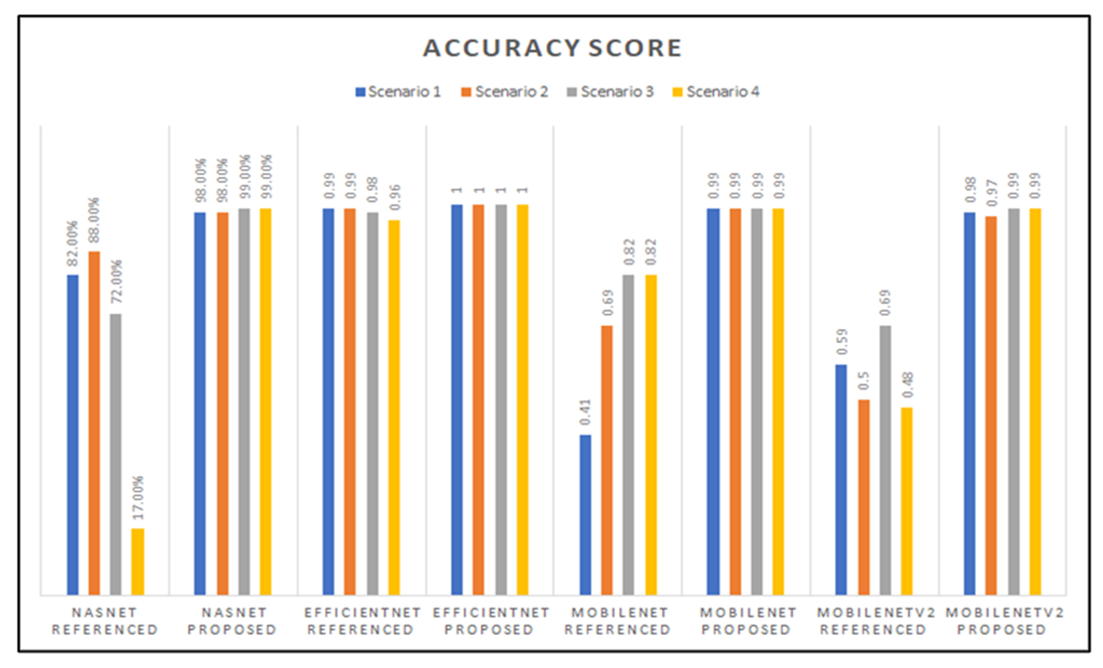
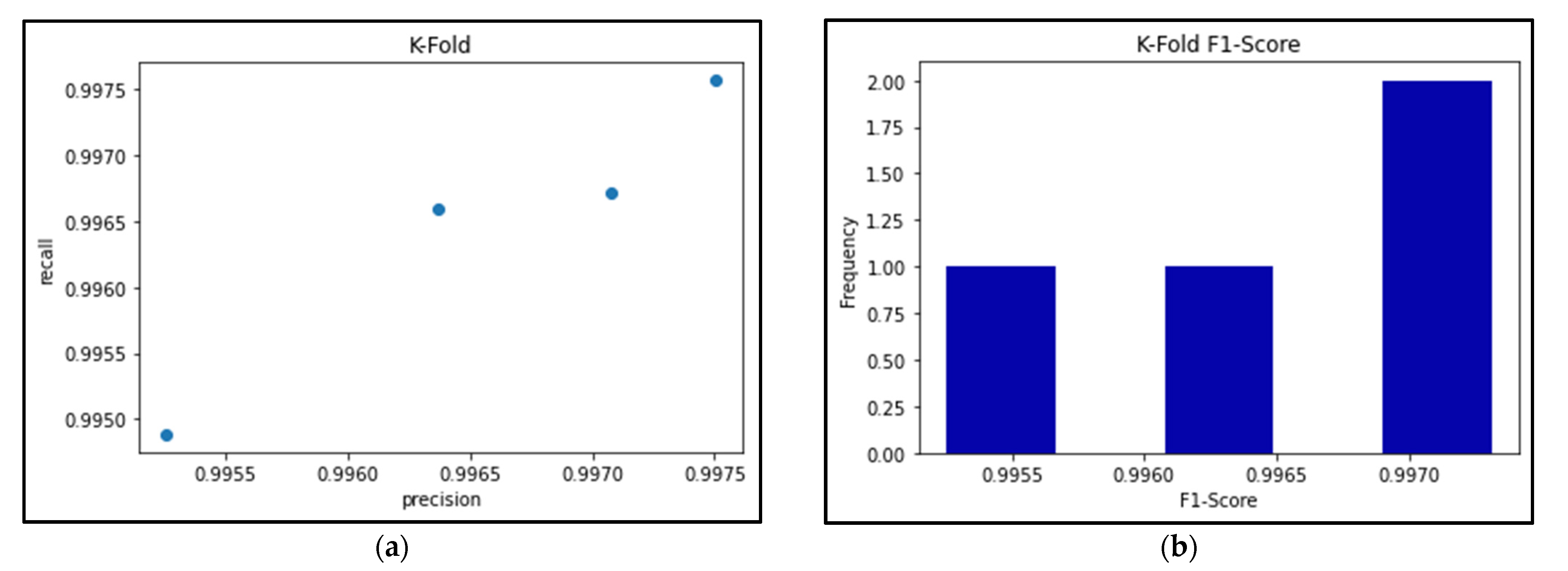
Overall, the best-performing model for our domain was concluded to be the fully retrained EfficientNetB0 base network (trained using the transfer learning Scenario 4 approach) using our improved proposed hyperparameters. This model had the most consistent top performance across our evaluated metrics, and these performance results were further supported by our K-fold cross validation evaluation, ensuring that the model confidently performed well with no data-split biases.
Beyond trying to find the best-performing model for the solution domain, our project also aimed to investigate the effects of using different CNN architectures, the effects of varying the retrained portions of the base networks, and the effects of varying the network hyperparameters on the models’ performances.
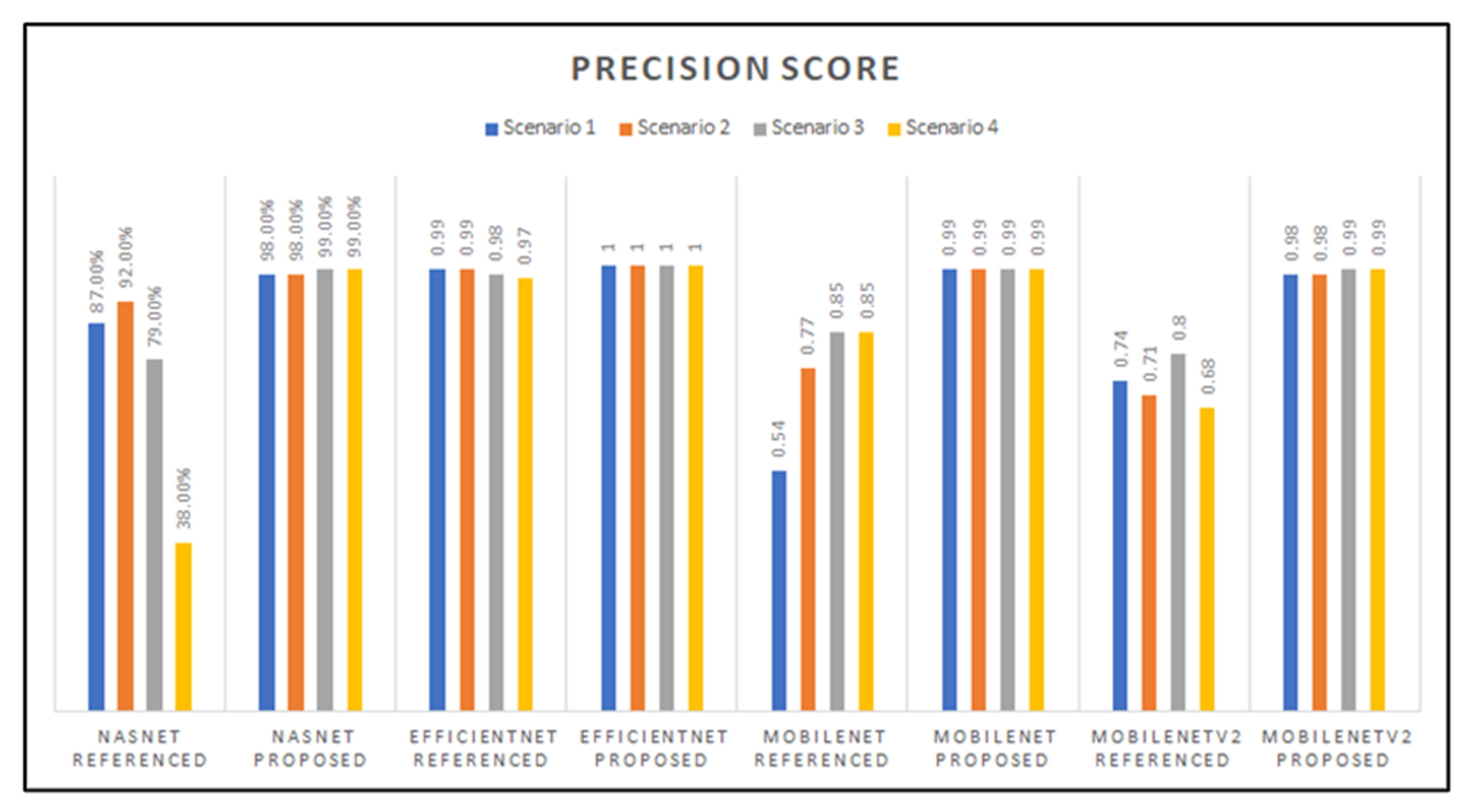
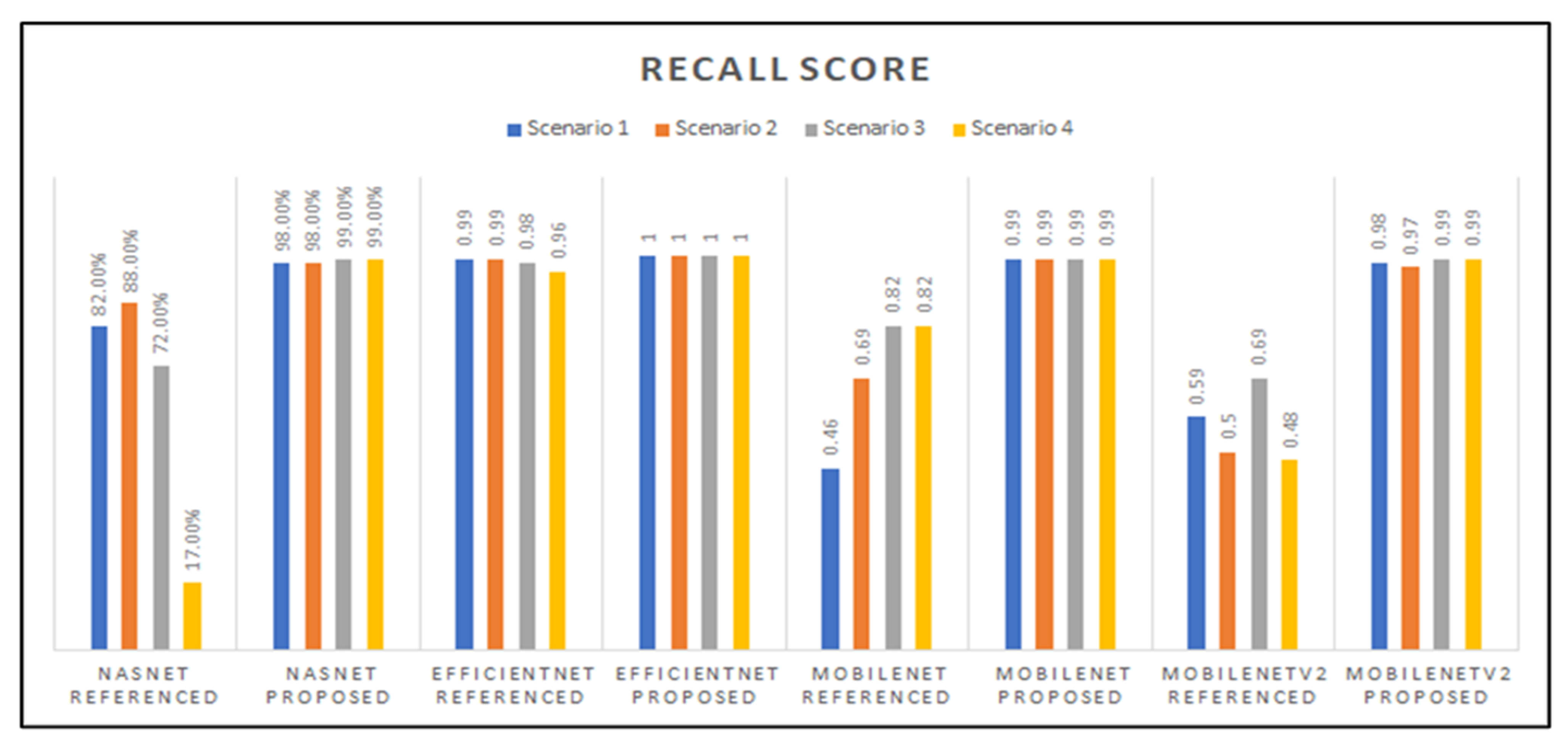
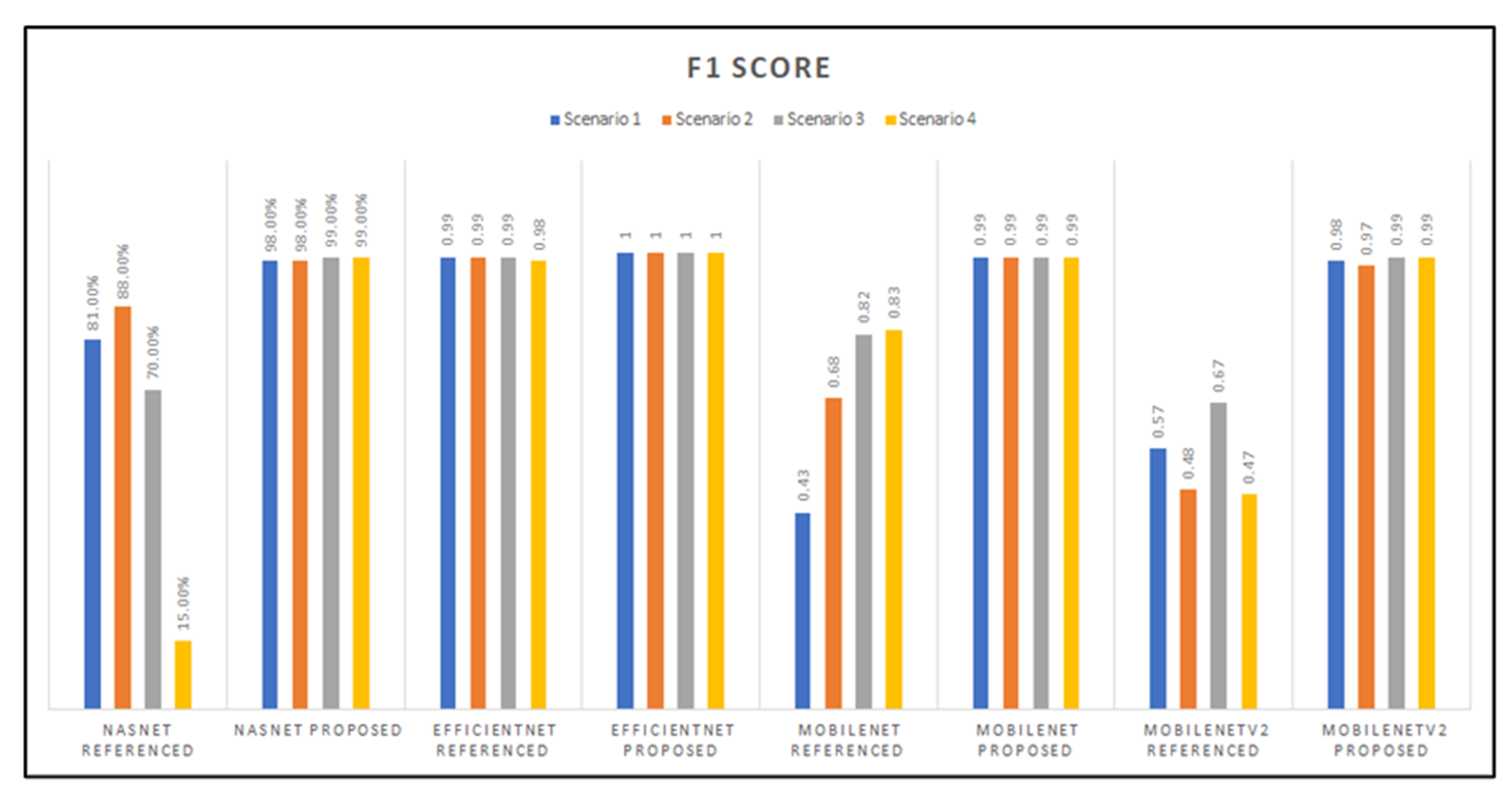
When investigating the effects of using different CNN architectures as the base-networks of our models, our findings show that the EfficientNetB0 model architecture frequently outperformed the MobileNetV2, MobileNet, and NasNetMobile models when considering the average scores and confusion matrices. The order of best- to worst-performing architectures were: EfficientNet; MobilNet; NasNetMobile; MobileNetV2.
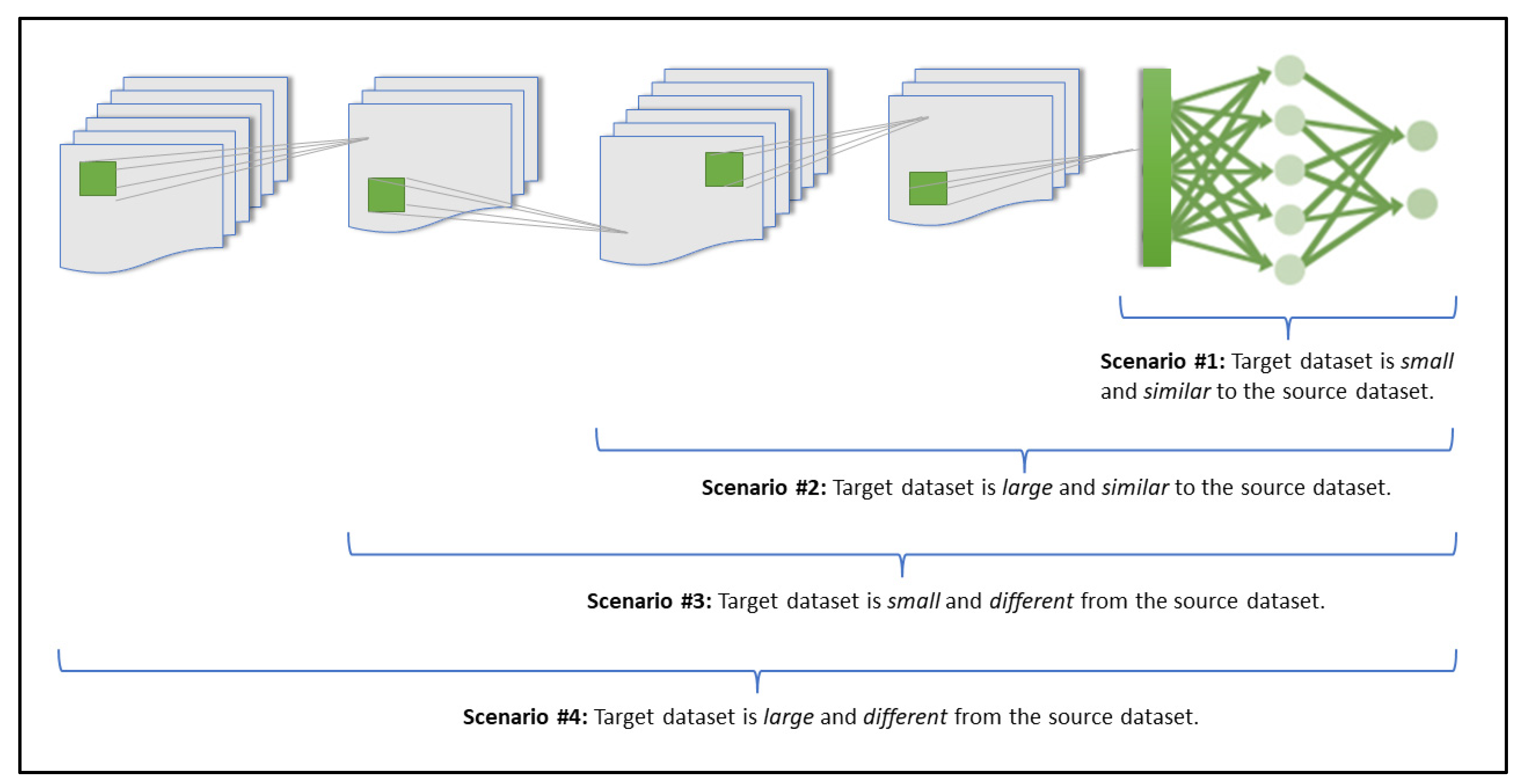
When investigating the effects of varying the retrained portions of the base networks (i.e., varying the transfer learning scenarios used), we observed that, across all the models,
Scenario 3 showed the best performance on average. This is evident as it never dropped below 67% for both the accuracy and F1-scores, and was always either the highest scoring or within 1% off the highest scoring model. This aligns with what we expected from a theoretical standpoint, as, according to [
20],
Scenario 3 (freezing the first half of the neural network and retraining the other half) is most useful when you have a target dataset that is smaller and of a relatively different domain to the pre-trained dataset. While the
ImageNet dataset that the base-network architecture is trained on includes millions of images and contains some images of plants and leaves, these images are not specifically of classified, close-up, diseased leaves, which means our dataset is considered to be of a relatively different domain and substantially smaller in size than the pre-trained source dataset, in turn falling within the recommended conditions of using
Scenario 3. On average,
Scenario 4 seems to trend as the worst-performing transfer learning scenario. This may be due to overfitting, as using a smaller dataset to fine-tune the entire base-network is often prone to overfitting the developed model as it becomes less able to generalize its learned features to new data. Meanwhile, our results show that
Scenario 2 performed better than
Scenario 1. This may be due to the difference in size between the pre-trained source dataset and our
PlantVillage dataset and how these sizes factor into the transfer learning scenarios.
When investigating the effects of varying the network hyperparameters on the models’ performances, our results show that our
proposed choice of hyperparameters—the learning rate, mini batch-size, and number of epochs—greatly improved the classification accuracy of the models. Using a smaller learning rate significantly improved results in comparison with initial results from [
19]. Additionally, our use of
Dropout layers for regularization helped avoid overfitting in the models, in contrast with some observed overfitting when using the initial (
referenced) hyperparameters from [
19]. By observing the difference between training and validation accuracies and losses, we can conclude that our models that used the
proposed hyperparameters were able to better generalize the learned features for new, unseen data. As such, we have achieved our intended goal of improving on the referenced models developed in [
19].
Our results indicate that the performance of the model depends on the model architecture and hyperparameters chosen as well as the portion of the network trained. Therefore, we have found that all three hypothesized factors (the model architecture, hyperparameter optimization, and the portion of the network retrained) can all each have a significant effect on the model performance.
5. Integrated System Implementation
To create our proposed mobile plant care support system for novice gardeners, we designed a simple-yet-comprehensive, three-tier solution consisting of a mobile application, a backend cloud database, and the aforementioned best-performing classification model. To maintain the desired lightweight portability and ease-of-access requirements of our system, we decided that an Android-based mobile application would be our primary touchpoint for the system, and that users would access all our implemented functionalities directly through the application. Our backend database was developed using Cloud Firestore to keep the system’s user-wide data stored in a centralized and secure fashion while simultaneously allowing for instances of user-specific data to also be stored and accessed using a similar backend process in the application. The mobile application is integrated with the respective deep learning classification model using a TensorFlow Lite file format and with the cloud database using the Cloud Firestore SDKs available for Android development. We chose to name the mobile app system “AgroAId” to present a clear and easy name that encompasses the system’s core values of agriculture, artificial intelligence (AI), identification, and plant care assistance (aid) in a unique, innovative, and simple manner.
5.1. Mobile Application Functionalities
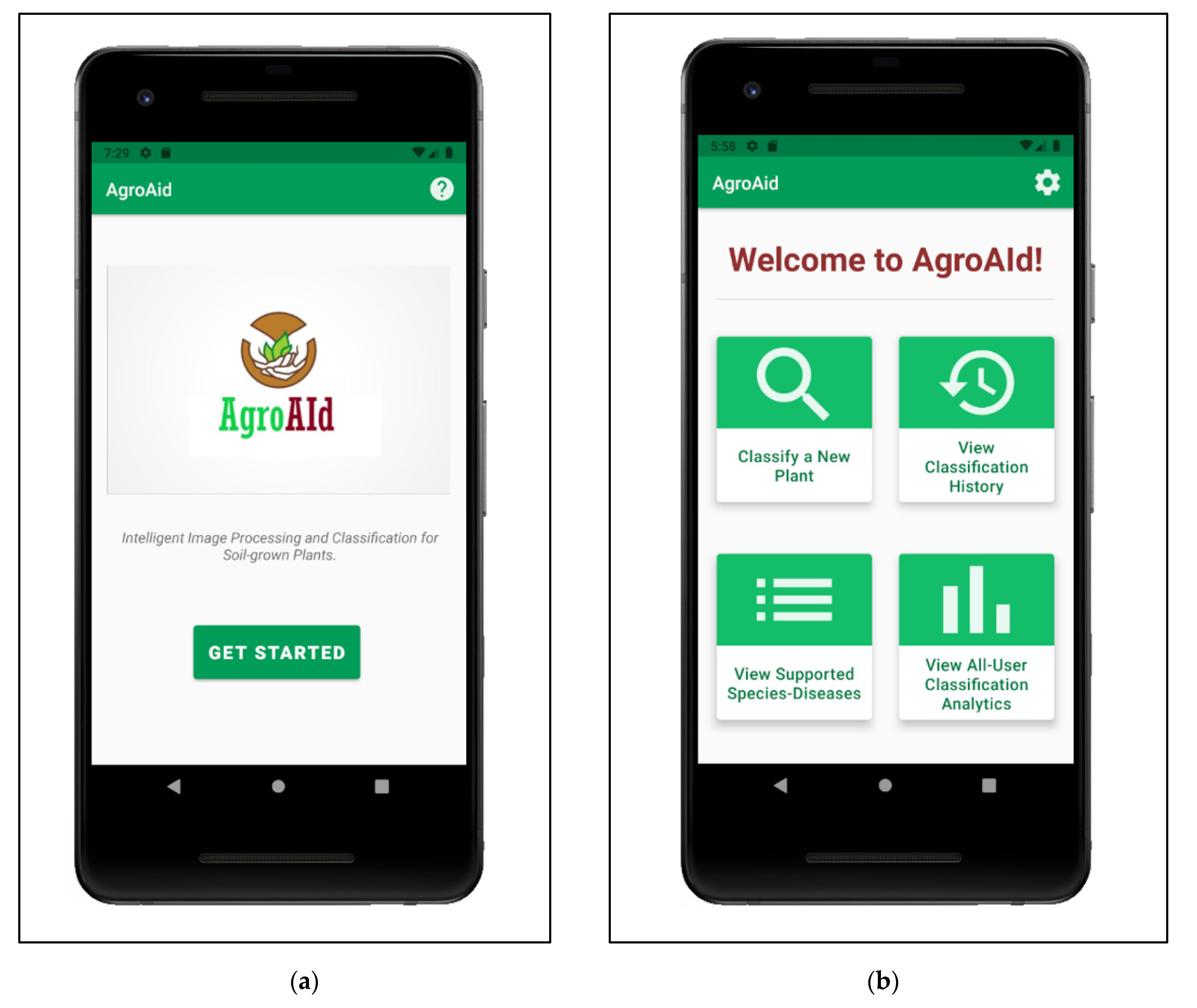
Maintaining a simple standard interface, the mobile application starts up on a minimal home page (
Figure 25a) that leads the user to a central activity (
Figure 25b) from which they can then access all the main system functionalities. The functionalities implemented in our system include:
Classifying a new input plant image based on the visual characteristics of its [species–disease] combination;
Retrieving and presenting the corresponding plant care details (e.g., symptoms and treatments) for the particular [species–disease] combination identified in an input image;
Storing and presenting a user-specific classification history;
Retrieving and presenting a list of all [species–disease] combinations supported by the system;
Configuring custom user settings pertaining to the user’s classification history and location region;
Retrieving and presenting user-wide spatiotemporal analytics about the system’s most commonly identified [species–disease] combinations filtered by season and region.
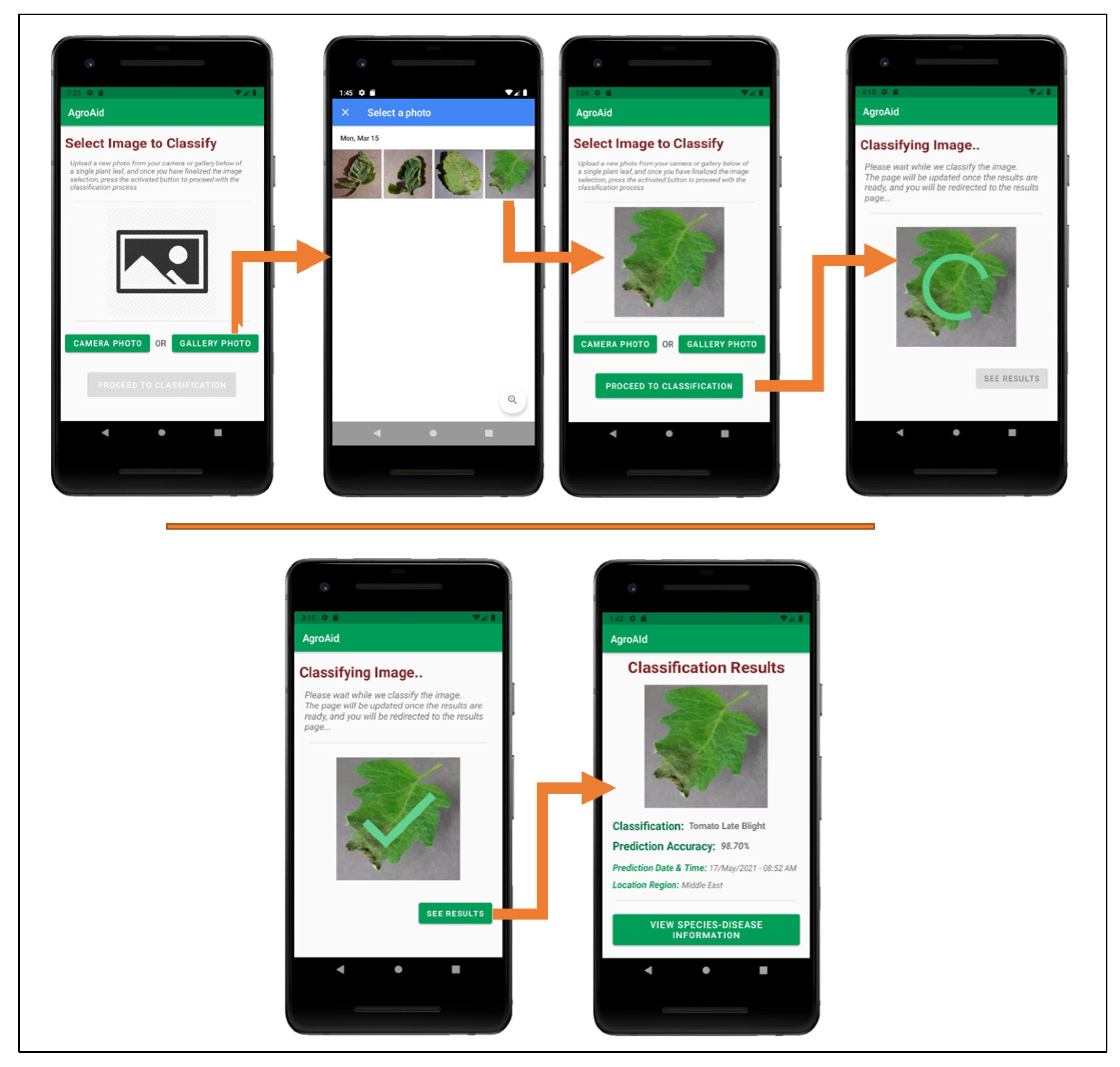
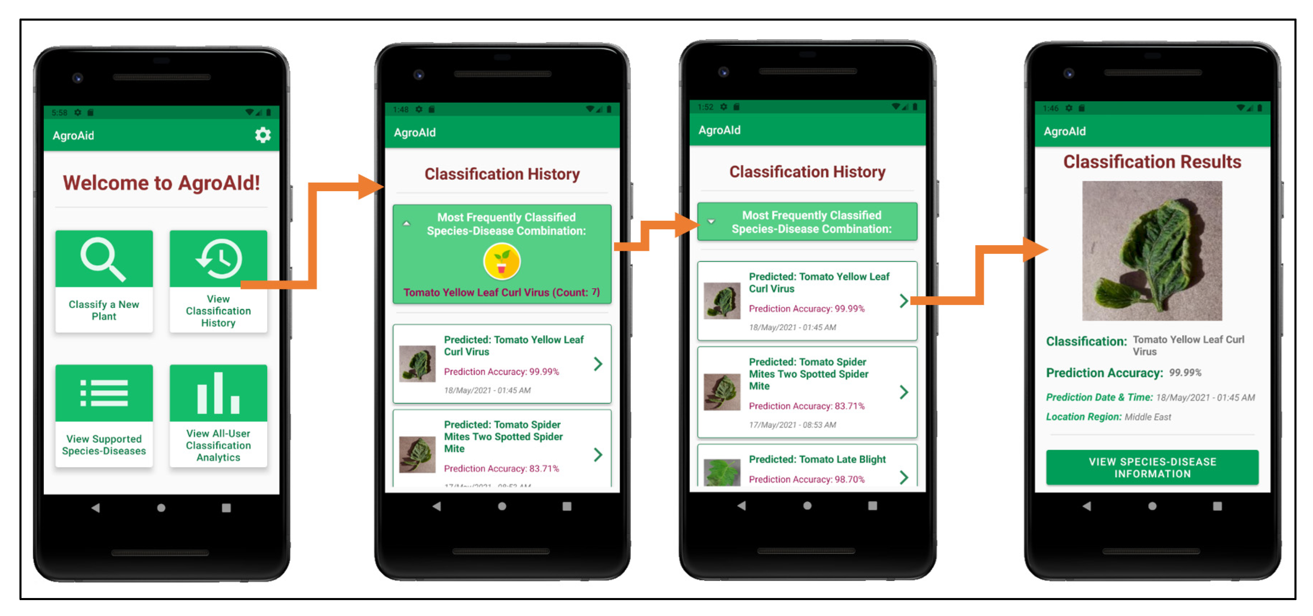
Figure 26 illustrates a walkthrough of the image classification functionality provided by our plant care support system as the user would experience it. The system’s classification functionality is initiated when the user selects to “Classify a New Plant” from the central activity in
Figure 26. From there, the user is directed to an image selection activity, where they can choose to input an image either using the device’s camera (i.e., taking a new photo) or the device’s gallery (i.e., uploading an existing stored image). Once the user confirms their selected image, an intermittent loading activity is displayed while the input image is classified in the background by the integrated deep learning model. Upon completing the classification, the results are displayed to the user in a dedicated results screen containing the classified image, predicted class label, prediction accuracy (confidence level), date and time of the classification, and the location region in which the user conducted the classification. The classification results are then stored in the system’s database under the user’s personal classification history, and the user-wide analytics are updated with the details of the identified class, location region, and season. The results screen also gives the user the choice to explore more plant-care information about the identified [
species–disease] combination.
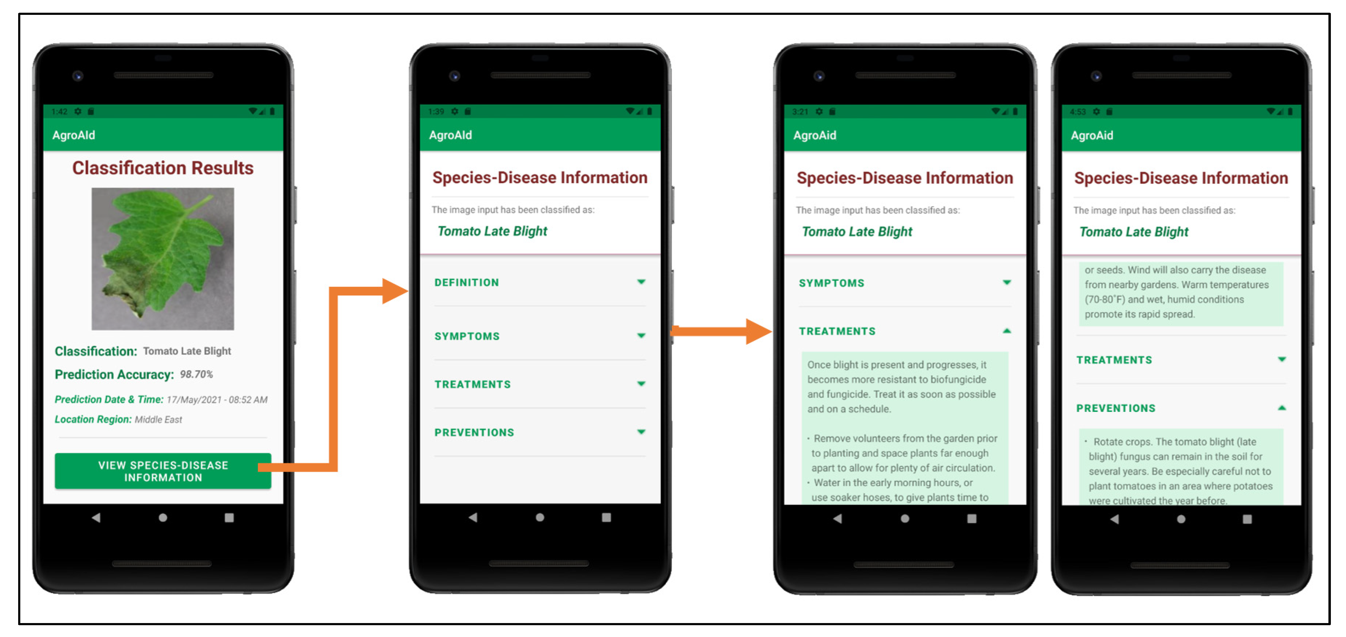
Figure 27 shows an example of the additional plant care support details provided to a user upon receiving a classification result; these details include the disease definition, symptoms, treatments, and future prevention for the particular [
species–disease]
combination identified. The plant care details were collected for every [
species–disease] combination recognized by the system to ensure that the user is provided with useful and accurate expert horticultural information for all of the system’s supported classification results. The information is stored in the centralized backend database to be accessible to all users and the details for the specific combination of interest are loaded in once the
Species–Disease Information activity is triggered via a call to the designated class responsible for all database operations. It is emphasized that the information presented is specific to the species-and-disease
combination as the same disease can have different symptoms or treatments depending on the species affected—this is a common, major pitfall that novice gardeners often face because they often do not possess the expert knowledge about the characteristics of particular species-and-disease combinations to know how to specifically treat them. As such, our application aims to provide the necessary information to guide gardeners to use plant care methods that are appropriate to the particular species and disease at hand in an attempt to make the plant care process easier and more effective.
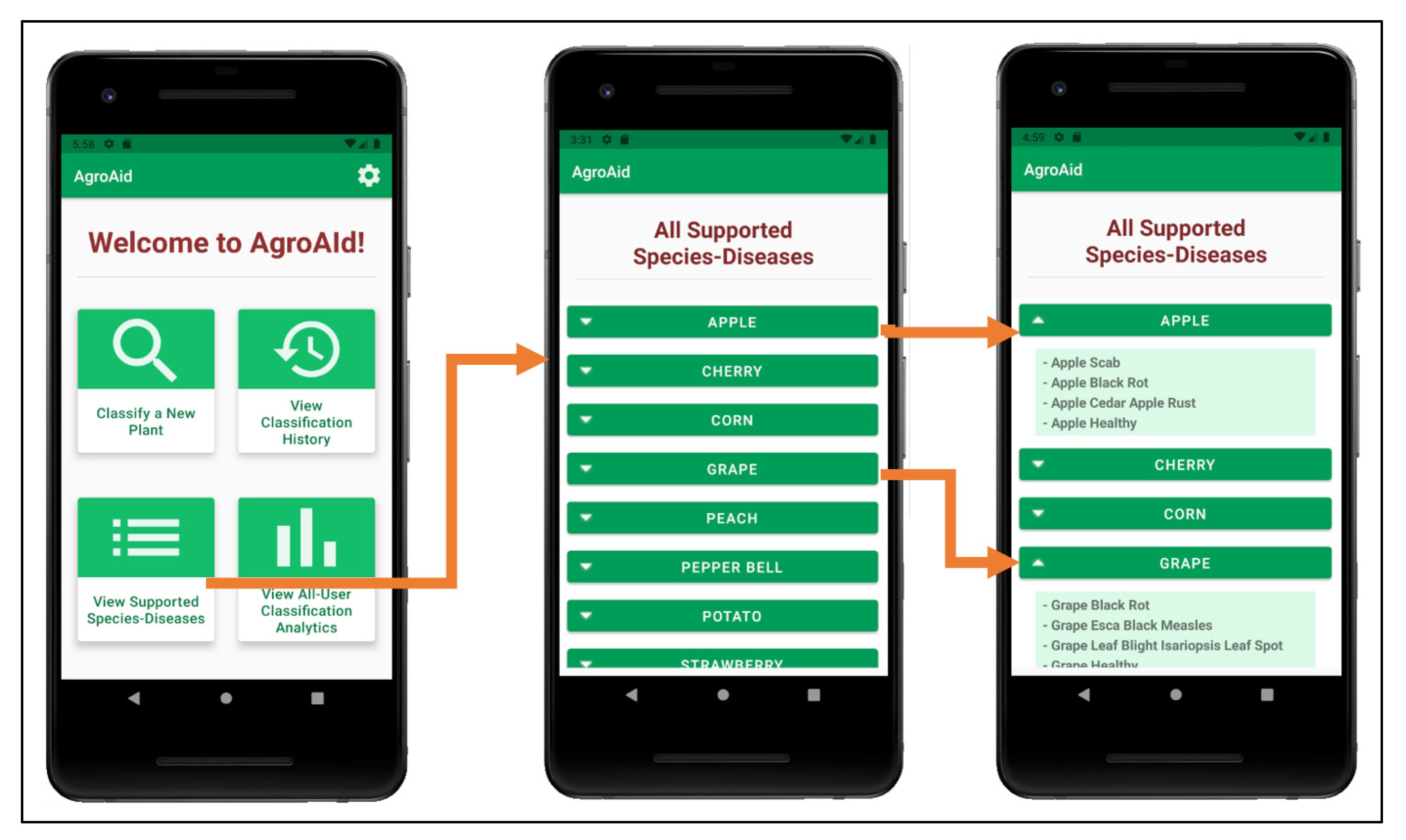
A user can view a full list of all the [
species–disease] combinations supported by the system from the central activity (
Figure 25b)—the supported combinations are those that the integrated AI model is able to recognize and classify. Having this feature available to users is necessary as the integrated model cannot identify all possible existing [
species–disease] combinations, meaning that an error in classifying an unsupported image is plausible. Therefore, presenting the list allows users to check if the plant species they wish to classify is supported and can minimize or help clarify any incorrect classifications that may occur as a result of inputting an image of an unsupported species/disease (see
Figure 28).
As the user continues to generate classification results using the system, they will accumulate their own collection of classification history records, which are stored in a user-specific sector of the system’s backend database and can be accessed by the user from the central activity (
Figure 25b). The
Classification History activity, as demonstrated in
Figure 29, lists the user’s past classification results chronologically from most-to-least recently classified and includes an initial preview of each record, including an icon-sized version of the classified image, the predicted class, the prediction accuracy, and the date and time of the classification. Each record card can then be expanded to see the full classification results page, and from there the user can optionally re-access the plant care information for that particular classification result, allowing them to refer back to the details at any time. The
Classification History activity also includes a distinguished minimizable card above the history records that displays the user’s most frequently classified [
species–disease] combination based on their classification history—this statistic can be useful for gardeners to learn if there is a particularly prominent common issue they are facing among their plants and as such allow them to seek a broader solution for treating it.
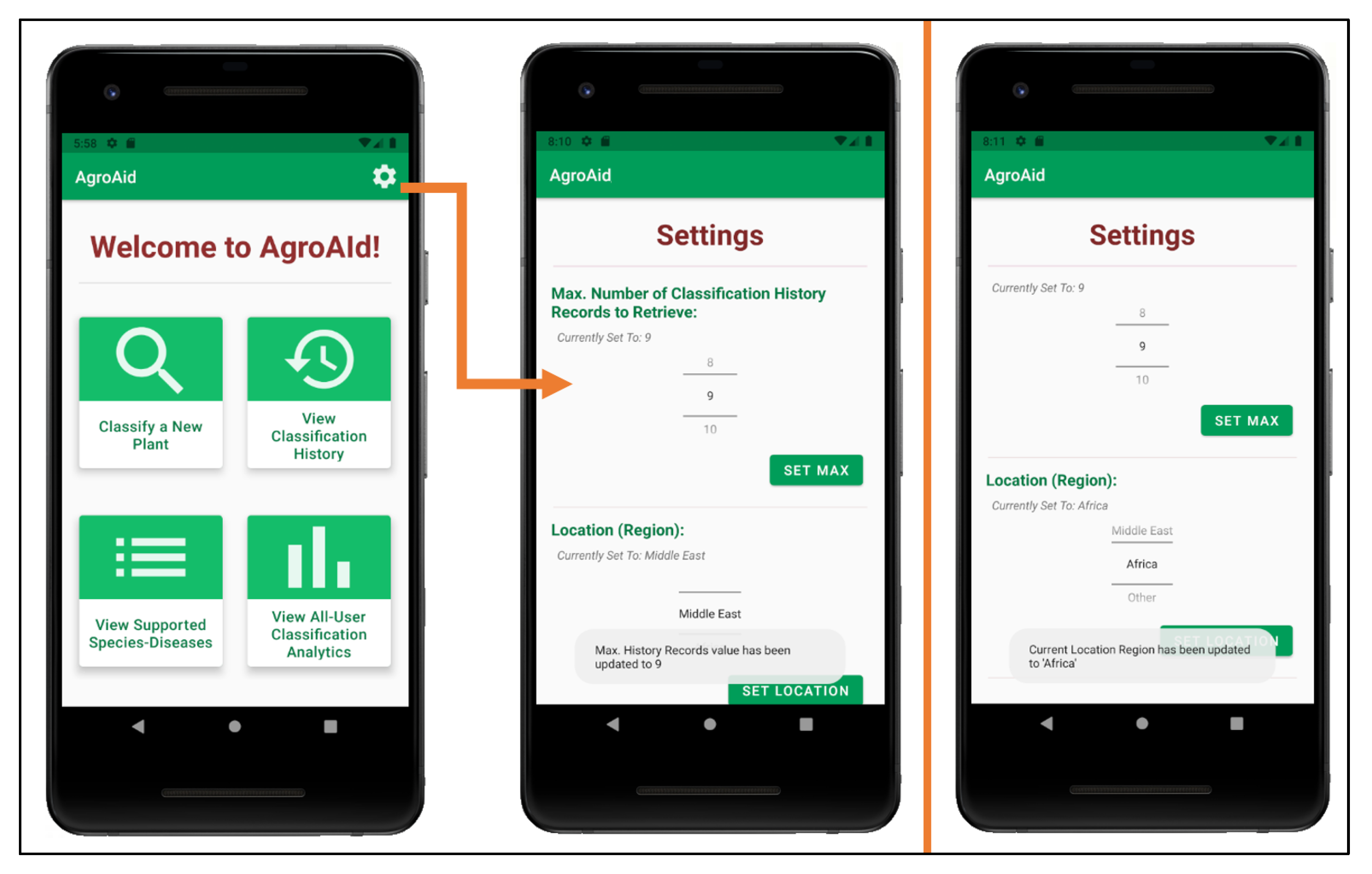
Custom app settings were developed for the system to allow users to flexibly configure their classification history and their location region (see
Figure 30). Users can select the maximum number of records they wish to see in their classification history list and the region from which they are conducting their classifications, the values of which are saved locally to the user’s device. The selected location region is used (along with the date and time of a classification) to update the system’s global analytics collection for each new classification result generated by a user.
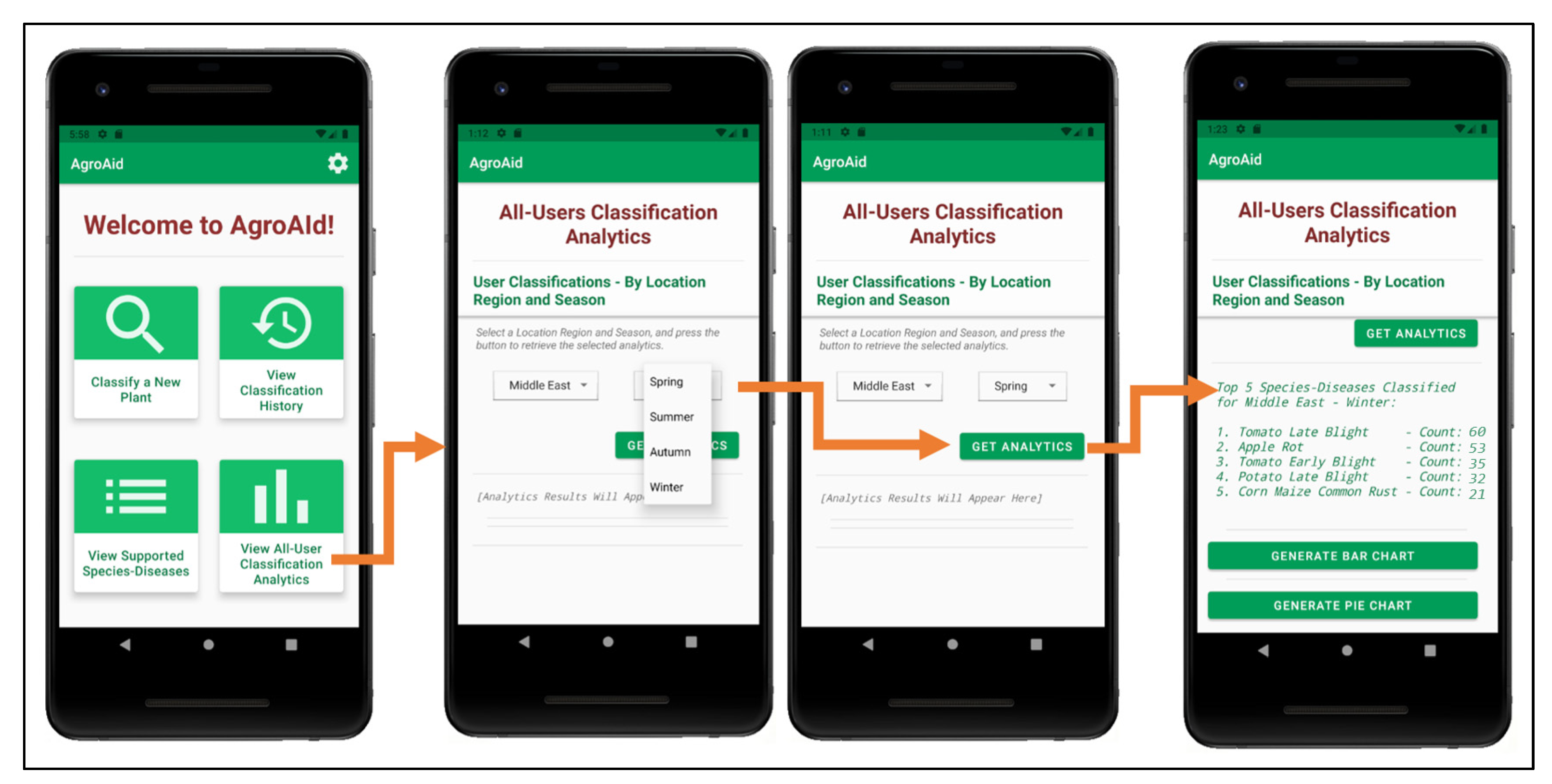
A unique feature included in our system is its ability to generate and present user-wide spatiotemporal analytics based on the users’ collective classification results—by considering the predicted class label, date, and location region of each classification conducted using our system, we can present the top, most commonly classified [species–disease] combinations filtered by region and season.
The data is stored in a dedicated centralized collection in the database that tallies the total count of classifications conducted with respect to their region, season, and identified [species–disease] combination. This global statistical data can be incredibly beneficial to gardeners to help them better understand the agricultural patterns that occur around them and how these external environmental or seasonal factors may be affecting their plants, in addition to generating new useful data about global agricultural trends that could then be used for future research in the field.
Within the application, users can access these analytics from the central activity, where they are directed to a screen that contains two drop-down filters to select the region and season of interest (see
Figure 31). Once the filters are selected and confirmed, the requested analytics are retrieved from the centralized backend database and the top 5 most commonly classified [
species–disease] combinations for the selected region and season are returned and displayed in the
Analytics activity.
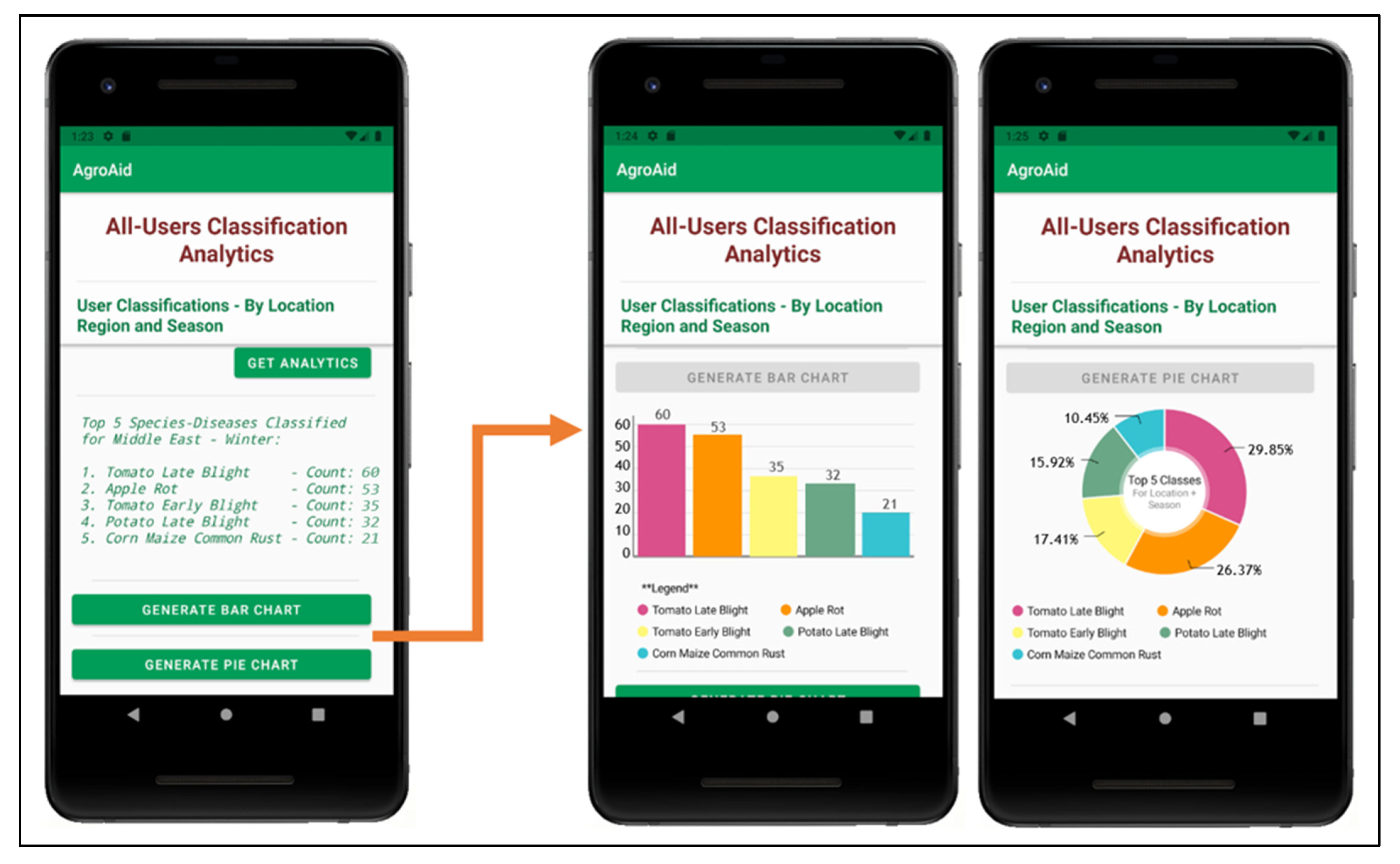
Beyond the textual results, the system also provides users the options to generate bar and pie charts of the analytics as an additional visualization of the statistics.
Figure 32 illustrates the respective bar and pie charts generated by the system for the same spatiotemporal analytics retrieved in
Figure 31. The open-source
MPAndroidChart library was used to create the base of the interactive chart views displayed in the application.
Author Contributions
Conceptualization, R.S., S.A., Y.R., and M.R.; methodology, S.A. and M.R.; software, M.R. and R.S.; validation, S.A. and Y.R.; formal analysis, R.S. and Y.R.; data curation, Y.R. and R.S.; writing—original draft preparation, M.R., S.A., Y.R. and R.S.; writing—review and editing, T.S., S.A. and M.R.; visualization, M.R. and R.S.; supervision, T.S.; project administration, T.S.; funding acquisition, Y.R. and S.A. All authors have read and agreed to the published version of the manuscript.
Funding
This research was supported in part by the American University of Sharjah, grant number URG21-001. This work is also supported in part by the Open Access Program from the American University of Sharjah. This paper represents the opinions of the authors and does not mean to represent the position or opinions of the American University of Sharjah.
Institutional Review Board Statement
Not applicable.
Informed Consent Statement
Not applicable.
Data Availability Statement
Conflicts of Interest
The authors declare no conflict of interest. The funders had no role in the design of the study; in the collection, analyses, or interpretation of data; in the writing of the manuscript; or in the decision to publish the results.
References
- Lu, J.; Tan, L.; Jiang, H. Review on convolutional neural network (CNN) applied to plant leaf disease classification. Agriculture 2021, 11, 707. [Google Scholar] [CrossRef]
- Ahmad, M.; Abdullah, M.; Moon, H.; Han, D. Plant disease detection in imbalanced datasets using efficient convolutional neural networks with stepwise transfer learning. IEEE Access 2021, 9, 140565–140580. [Google Scholar] [CrossRef]
- O’Mahony, N.; Campbell, S.; Carvalho, A.; Harapanahalli, S.; Hernandez, G.V.; Krpalkova, L.; Riordan, D.; Walsh, J. Deep learning vs. traditional computer vision. Adv. Intell. Syst. Comput. 2019, 943, 128–144. [Google Scholar] [CrossRef] [Green Version]
- Elsayed, E.; Aly, M. Hybrid between ontology and quantum particle swarm optimization for segmenting noisy plant disease image Int. J. Syst. Appl. Eng. Dev. 2020, 14, 71–80. [Google Scholar] [CrossRef]
- Asefpour Vakilian, K.; Massah, J. An artificial neural network approach to identify fungal diseases of cucumber (Cucumis sativus L.) plants using digital image processing. Arch. Phytopathol. PlantProt. 2013, 46, 1580–1588. [Google Scholar] [CrossRef]
- Yang, J.; Bagavathiannan, M.; Wang, Y.; Chen, Y.; Yu, J. A comparative evaluation of convolutional neural networks, training image sizes, and deep learning optimizers for weed detection in Alfalfa. Weed Technol. 2022, 1–30. [Google Scholar] [CrossRef]
- Shaji, A.P.; Hemalatha, S. Data augmentation for improving rice leaf disease classification on residual network architecture. Int. Conf. Adv. Comput. Commun. Appl. Inform. (ACCAI) 2022, 1–7. [Google Scholar] [CrossRef]
- Chen, J.; Chen, W.; Zeb, A.; Yang, S.; Zhang, D. Lightweight inception networks for the recognition and detection of rice plant diseases. IEEE Sens. J. 2022, 22, 14628–14638. [Google Scholar] [CrossRef]
- Liu, J.; Wang, X. Early recognition of tomato gray leaf spot disease based on MobileNetv2-YOLOv3 model. Plant. Methods 2020, 16. [Google Scholar] [CrossRef]
- Ma, J.; Du, K.; Zheng, F.; Zhang, L.; Gong, Z.; Sun, Z. A recognition method for cucumber diseases using leaf symptom images based on deep convolutional neural network. Comput. Electron. Agric. 2018, 154, 18–24. [Google Scholar] [CrossRef]
- Sagar, A.; Dheeba, J. On using transfer learning for plant disease detection. bioRxiv 2020. [Google Scholar] [CrossRef]
- Altuntaş, Y.; Kocamaz, F. Deep feature extraction for detection of tomato plant diseases and pests based on leaf images. Celal Bayar Üniv. Fen Bilim. Derg. 2021, 17, 145–157. [Google Scholar] [CrossRef]
- Rao, D.S.; Babu Ch, R.; Kiran, V.S.; Rajasekhar, N.; Srinivas, K.; Akshay, P.S.; Mohan, G.S.; Bharadwaj, B.L. Plant disease classification using deep bilinear CNN. Intell. Autom. Soft Comput. 2022, 31, 161–176. [Google Scholar] [CrossRef]
- Dammavalam, S.R.; Challagundla, R.B.; Kiran, V.S.; Nuvvusetty, R.; Baru, L.B.; Boddeda, R.; Kanumolu, S.V. Leaf image classification with the aid of transfer learning: A deep learning approach. Curr. Chin. Comput. Sci. 2021, 1, 61–76. [Google Scholar] [CrossRef]
- Chethan, K.S.; Donepudi, S.; Supreeth, H.V.; Maani, V.D. Mobile application for classification of plant leaf diseases using image processing and neural networks. Data Intell. Cogn. Inform. 2021, 287–306. [Google Scholar] [CrossRef]
- Valdoria, J.C.; Caballeo, A.R.; Fernandez, B.I.D.; Condino, J.M.M. iDahon: An Android based terrestrial plant disease detection mobile application through digital image processing using deep learning neural network algorithm. In Proceedings of the 2019 4th International Conference on Information Technology (InCIT), Bangkok, Thailand, 24–25 October 2019. [Google Scholar]
- Ahmad, J.; Jan, B.; Farman, H.; Ahmad, W.; Ullah, A. Disease detection in plum using convolutional neural network under true field conditions. Sensors 2020, 20, 5569. [Google Scholar] [CrossRef]
- Reda, M.; Suwwan, R.; Alkafri, S.; Rashed, Y.; Shanableh, T. A mobile-based novice agriculturalist plant care support system: Classifying plant diseases using deep learning. In Proceedings of the 2021 12th International Conference on Information and Communication Systems (ICICS), Valencia, Spain, 24–26 May 2021. [Google Scholar]
- Syamsuri, B.; Negara, I. Plant disease classification using Lite pretrained deep convolutional neural network on Android mobile device. Int. J. Innov. Technol. Explor. Eng. 2019, 9, 2796–2804. [Google Scholar] [CrossRef]
- Elgendy, M. Deep Learning for Vision Systems; Manning Publications: Shelter Island, NY, USA, 2020; pp. 240–262. [Google Scholar]
- Zhuang, F.; Qi, Z.; Duan, K.; Xi, D.; Zhu, Y.; Zhu, H.; Xiong, H.; He, Q. A comprehensive survey on transfer learning. Proc. IEEE 2021, 109, 43–76. [Google Scholar] [CrossRef]
- Barbedo, J.G.A. Impact of dataset size and variety on the effectiveness of deep learning and transfer learning for plant disease classification. Comput. Electron. Agric. 2018, 153, 46–53. [Google Scholar] [CrossRef]
- Geetharamani, G.; Arun Pandian, J. Identification of plant leaf diseases using a 9-layer deep convolutional neural network. Comput. Electr. Eng. 2019, 76, 323–338. [Google Scholar] [CrossRef]
- Howard, A.G.; Zhu, M.; Chen, B.; Kalenichenko, D.; Wang, W.; Weyand, T.; Andreetto, M.; Adam, H. Mobilenets: Efficient convolutional neural networks for mobile vision applications. arXiv 2017. [Google Scholar] [CrossRef]
- Sandler, M.; Howard, A.; Zhu, M.; Zhmoginov, A.; Chen, L.C. MobileNetV2: Inverted residuals and linear bottlenecks. In Proceedings of the 2018 IEEE/CVF Conference on Computer Vision and Pattern Recognition (CVPR), Salt Lake City, UT, USA, 18–23 June 2018. [Google Scholar]
- Tan, M.; Chen, B.; Pang, R.; Vasudevan, V.; Sandler, M.; Howard, A.; Le, Q.V. MnasNet: Platform-aware neural architecture search for mobile, In Proceedings of 2019 IEEE/CVF Conference on Computer Vision and Pattern Recognition (CVPR), Long Beach, CA, USA, 15-20 June 2019.
- EfficientNet: Rethinking Model Scaling for Convolutional Neural Networks. Available online: https://proceedings.mlr.press/v97/tan19a.html (accessed on 20 May 2022).
- EfficientNet: Improving Accuracy and Efficiency through AutoML and Model Scaling. Google AI Blog. 2019. Available online: https://ai.googleblog.com/2019/05/efficientnet-improving-accuracy-and.html (accessed on 20 May 2022).
- Get Started with TensorFlow Lite. Available online: https://www.tensorflow.org/lite/guide (accessed on 20 May 2022).
- TensorFlow Lite: Model Conversion Overview. Available online: https://www.tensorflow.org/lite/models/convert (accessed on 20 May 2022).
Figure 1.
The four transfer learning scenarios and their respective fine-tuning guidelines (inspired by [
20]).
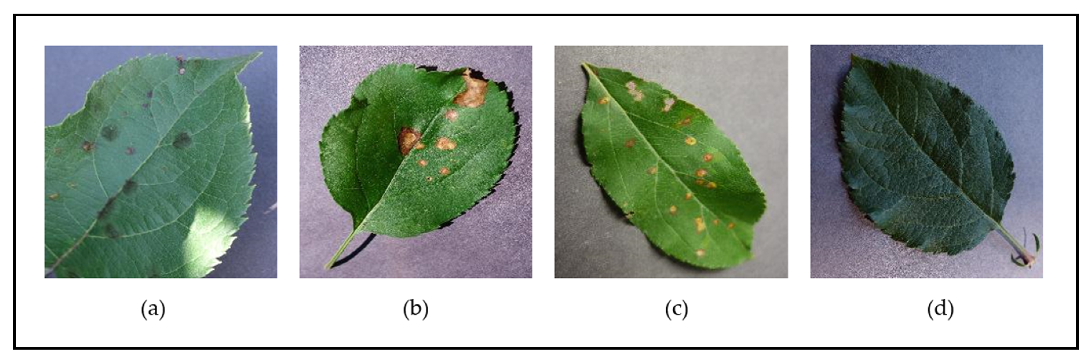
Figure 2.
Examples of leaves from the different classes supported for the Apple species in the PlantVillage dataset—(a) Apple Scab; (b) Apple Black Rust; (c) Apple Cedar Rot; (d) Apple Healthy.
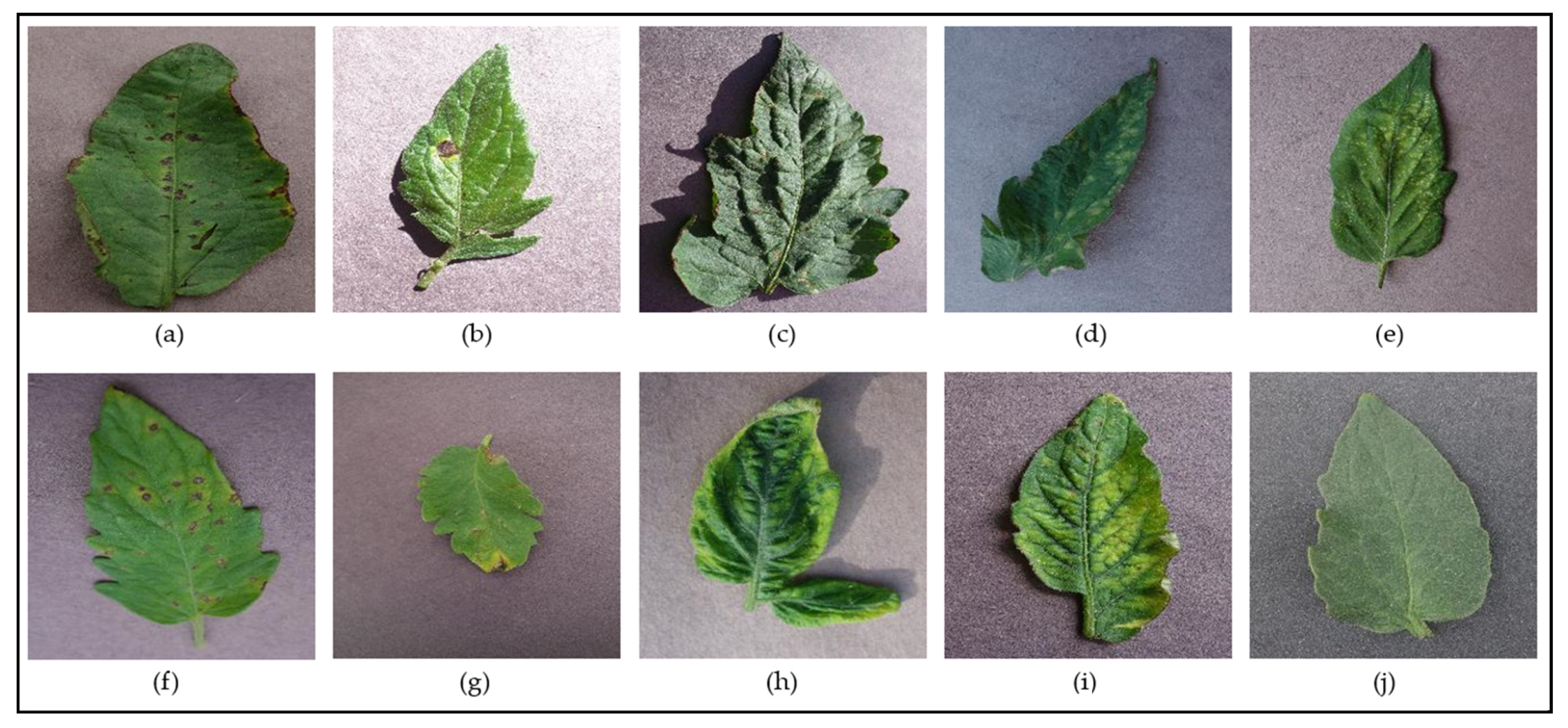
Figure 3.
Examples of leaves from the different classes supported for the Tomato species in the PlantVillage dataset—(a) Tomato Bacterial Spot; (b) Tomato Early Blight; (c) Tomato Target Spot; (d) Tomato Leaf Mold; (e) Tomato Two-Spotted Spider Mite; (f) Tomato Septoria Leaf Spot; (g) Tomato Late Blight; (h) Tomato Yellow-Leaf Curl Virus; (i) Tomato Mosaic Virus; (j) Tomato Healthy.
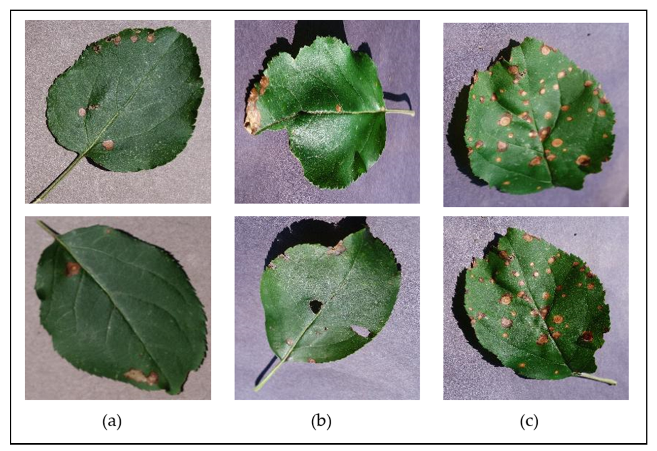
Figure 4.
Examples of some of the different leaf states represented in the dataset, shown for the “Apple Black Rot” class—(a) early symptoms, on a flat, complete leaf; (b) moderate symptoms, on a slightly distressed leaf; (c) severe symptoms, on a slightly bent, complete leaf.
Figure 5.
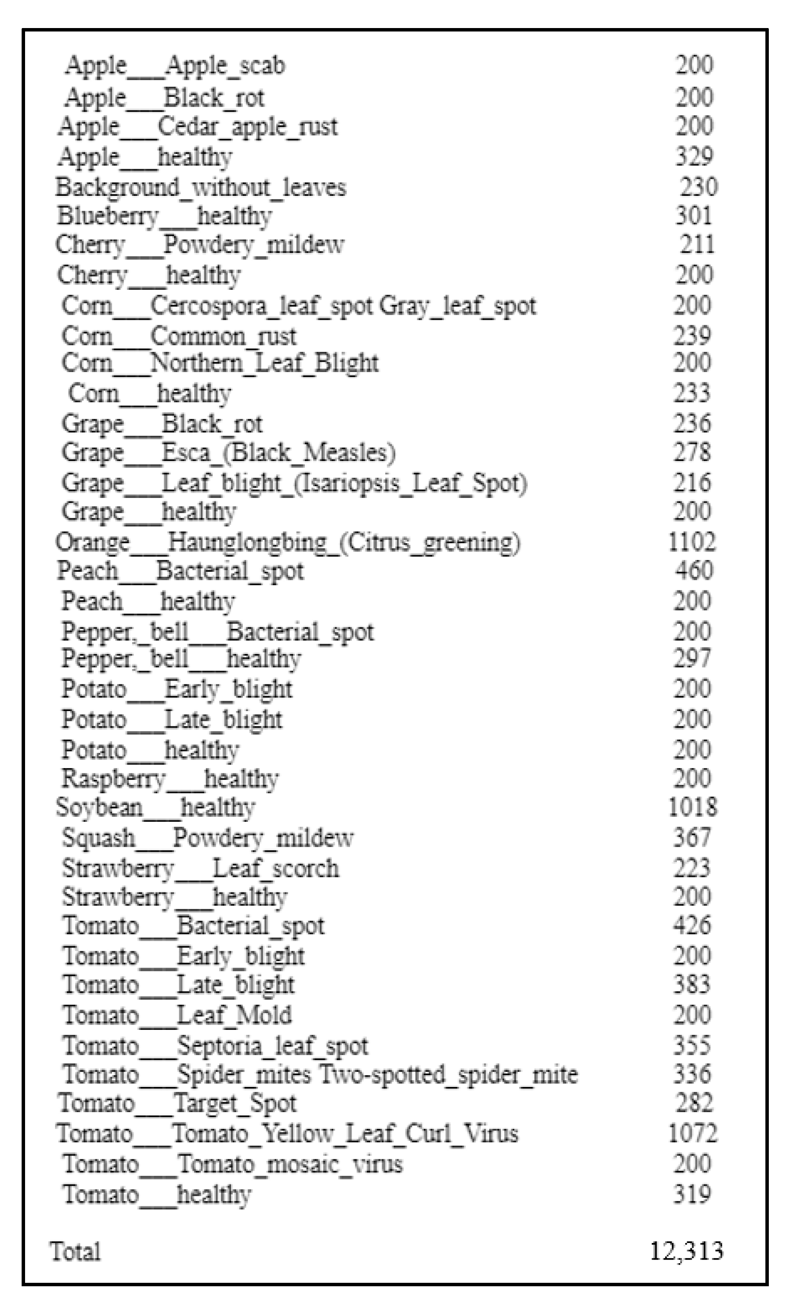
The dataset split for the testing subset of images, with the number of testing images used for each classification label (total 39 labels).
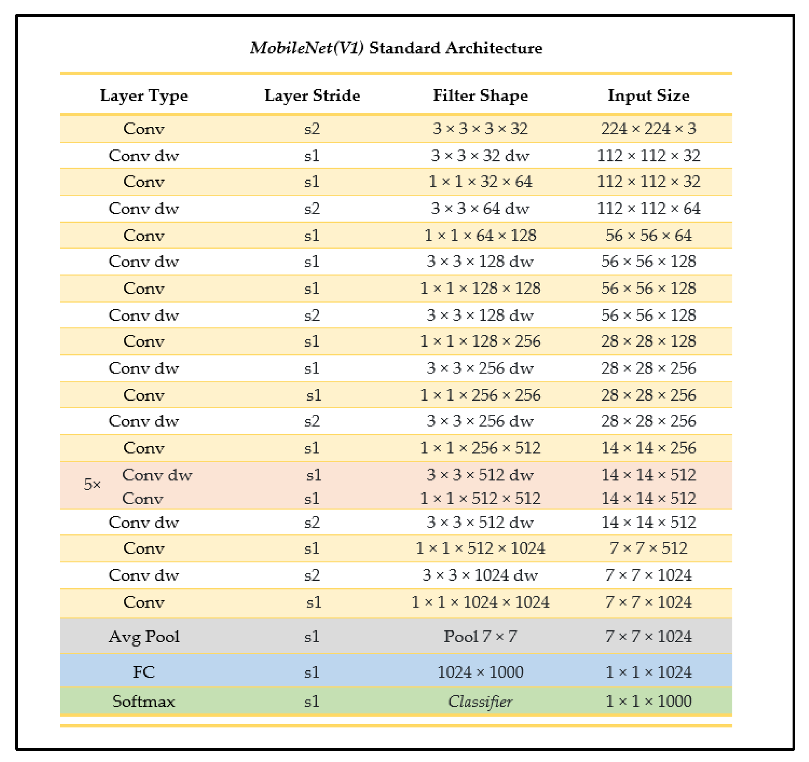
Figure 6.
MobileNet standard architecture (as outlined in [
24]).
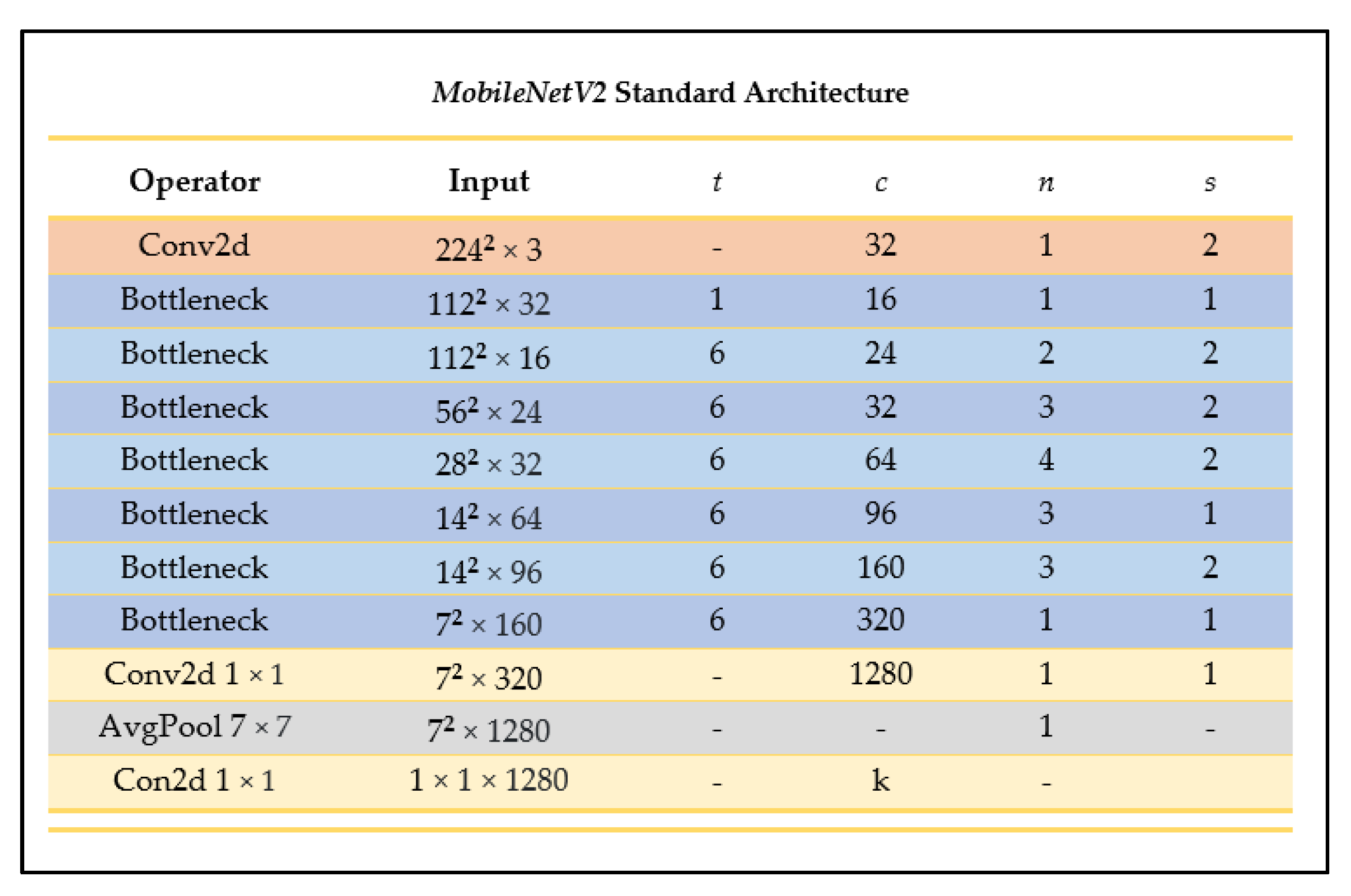
Figure 7.
MobileNetV2 architecture summary (as outlined in [
25]).
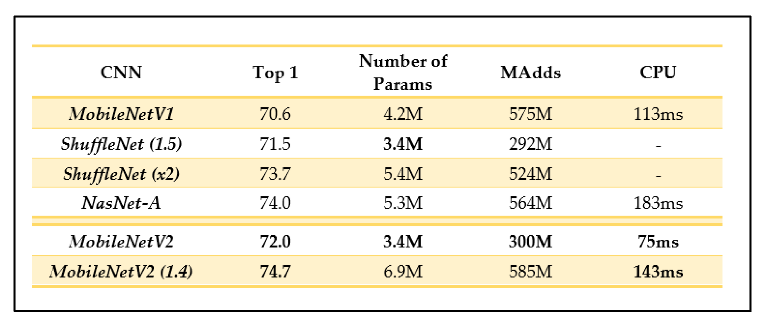
Figure 8.
Comparison of
MobileNetV2 results and other recent CNN architectures (as outlined in [
25]).
Figure 9.
Visual overview of
NasNetMobile architecture (as described in [
26]).
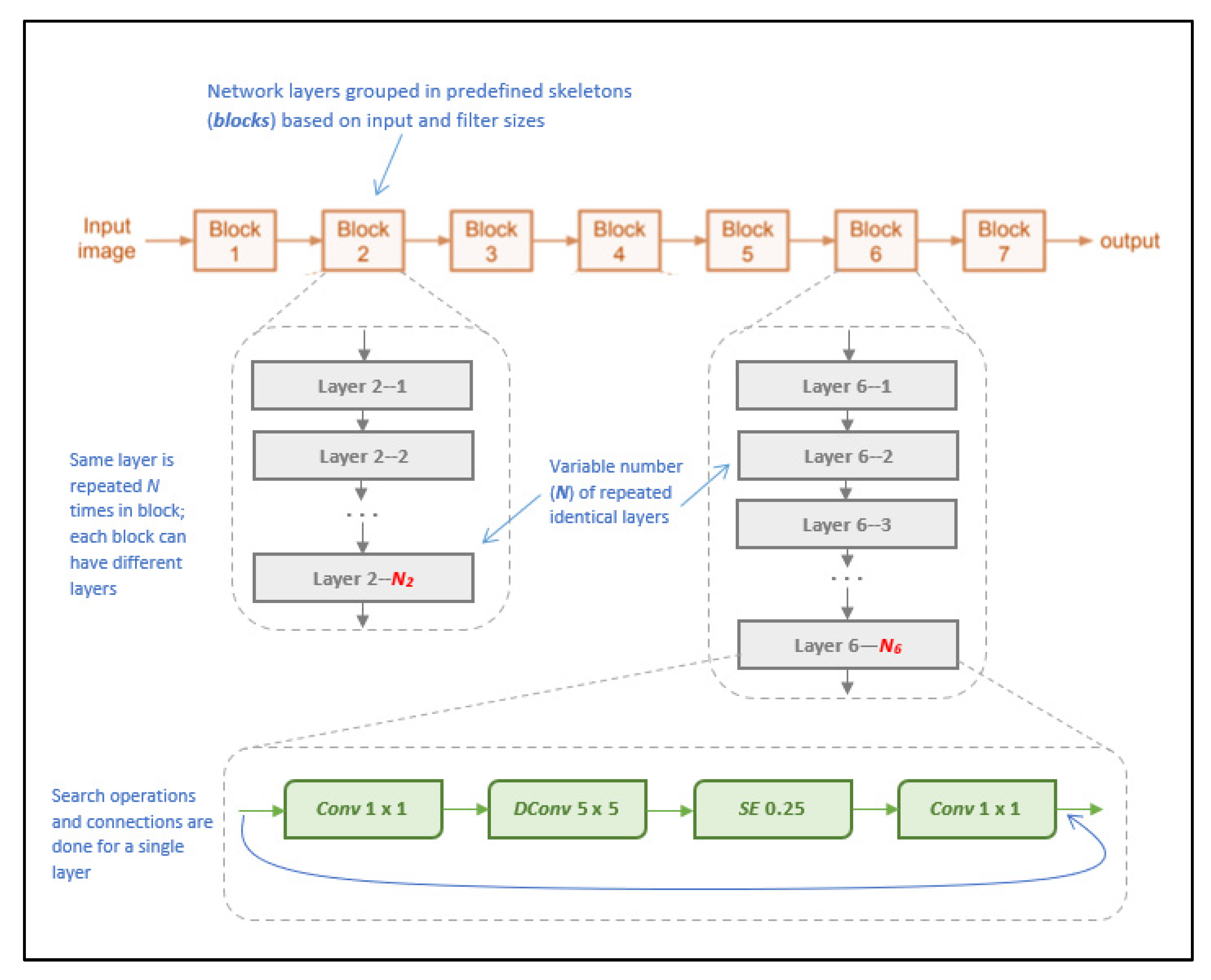
Figure 10.
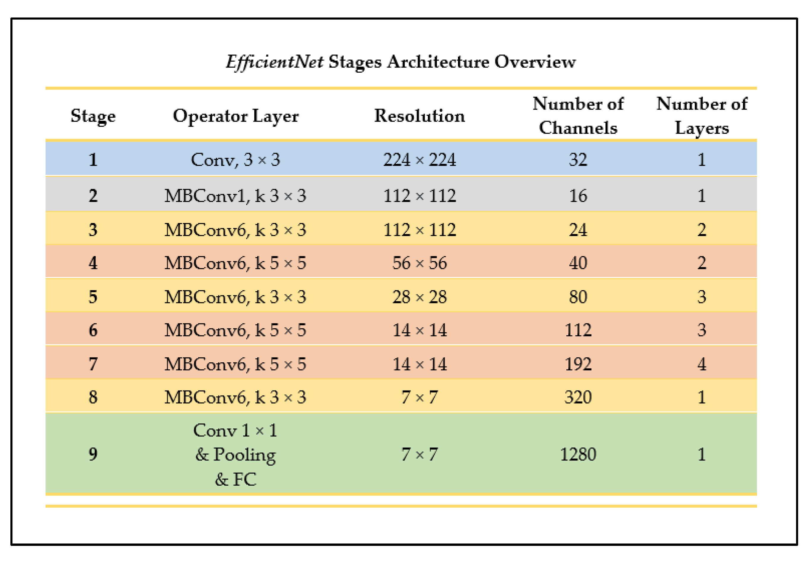
Architecture overview of
EfficientNet (as outlined in [
27]).
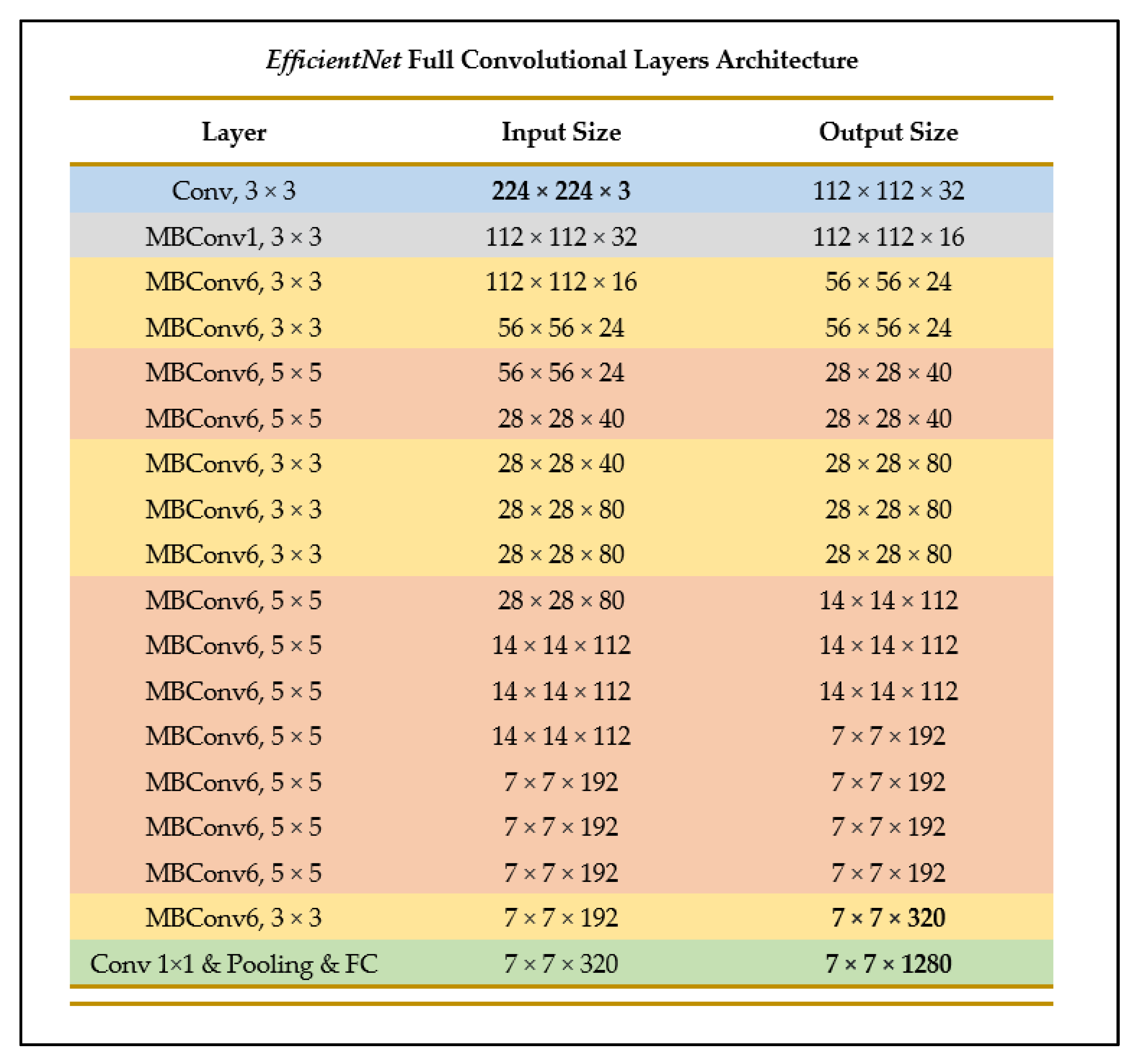
Figure 11.
Breakdown of convolutional layers of
EfficientNet (as outlined in [
27]).
Figure 12.
Graphed results of accuracy scores for all models developed.
Figure 13.
Graphed results of precision score for all models developed.
Figure 14.
Graphed results of recall scores for all models developed.
Figure 15.
Graphed results of F1-scores for all models developed.
Figure 16.
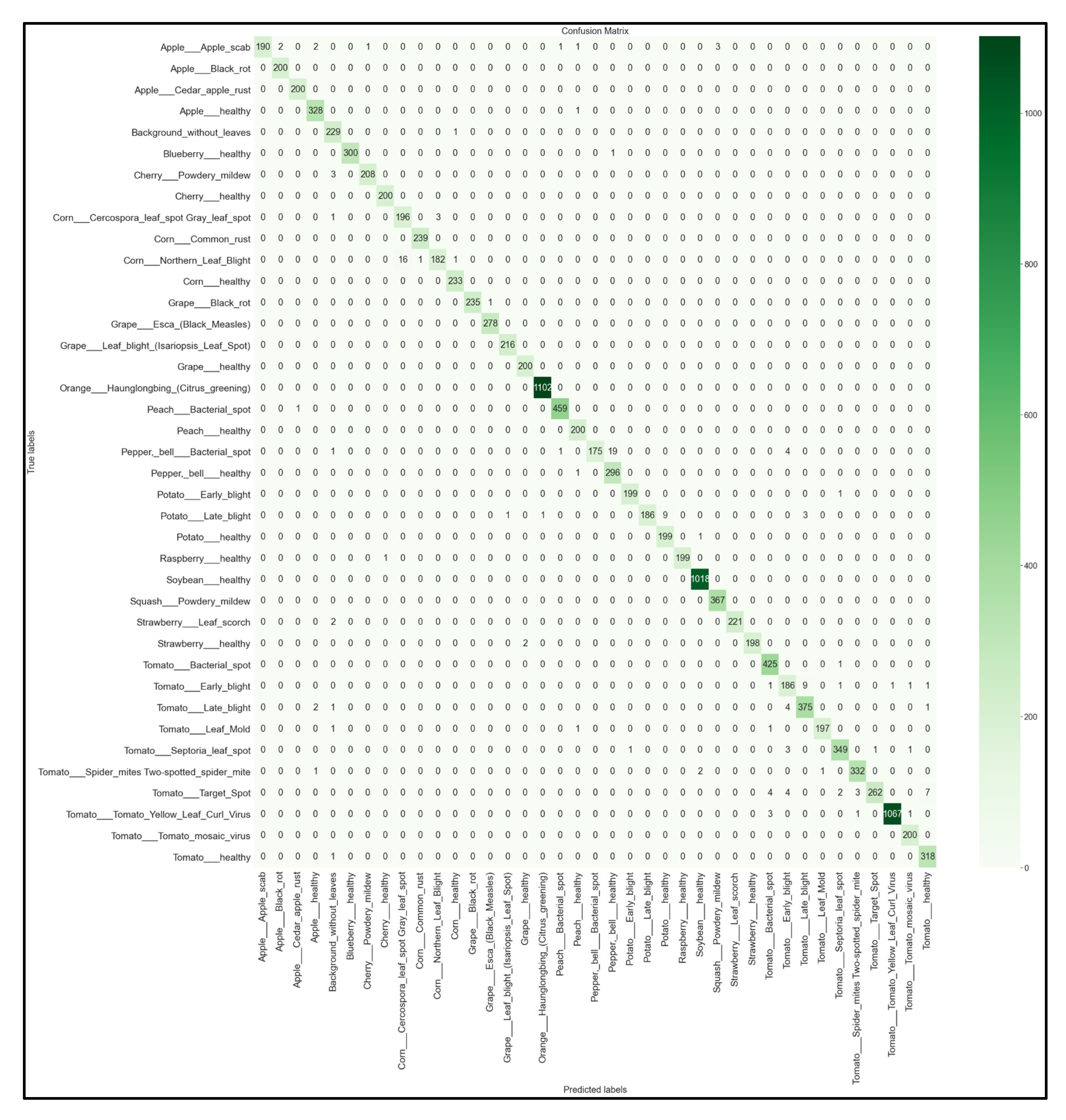
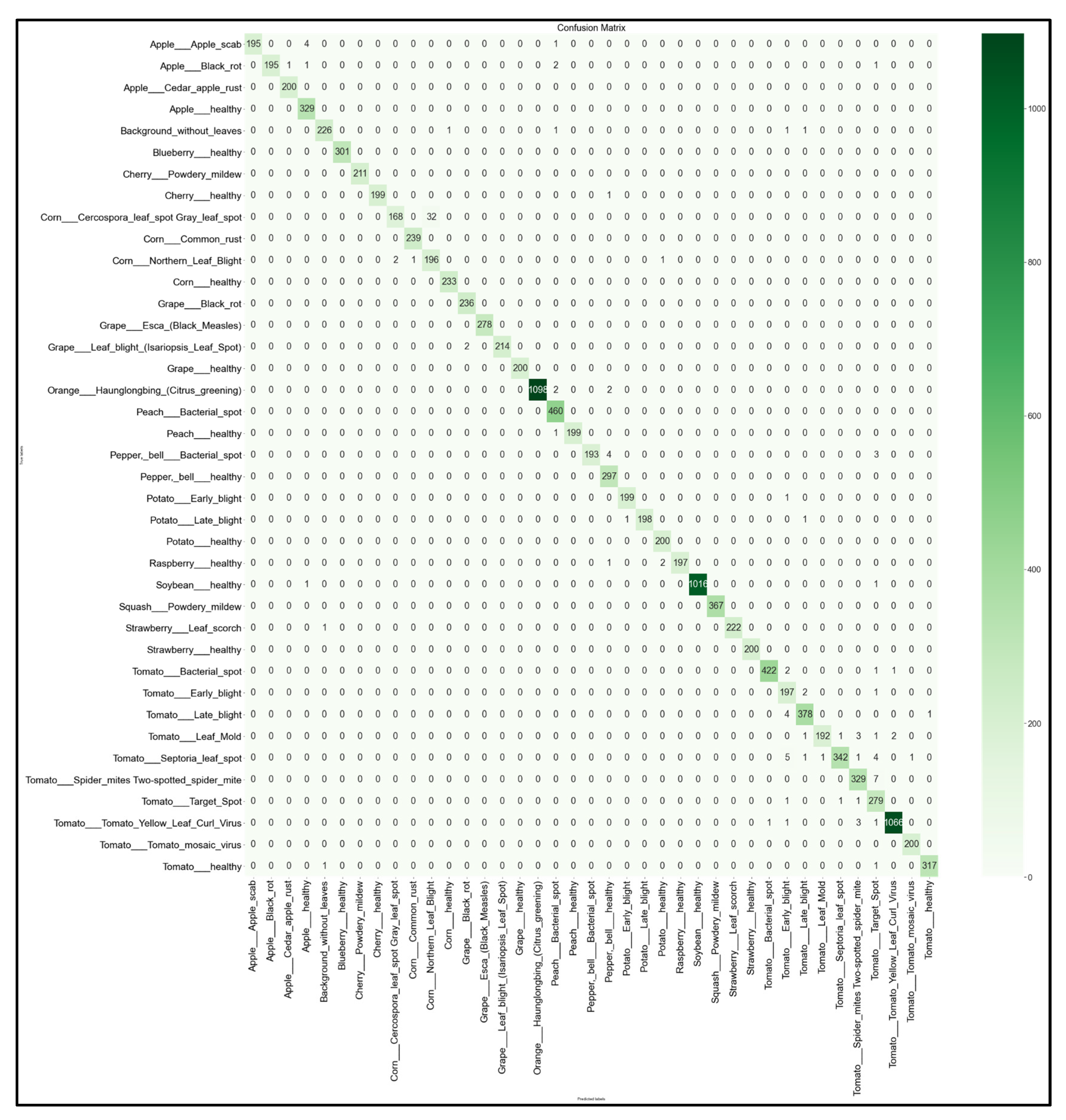
39 × 39 Confusion matrix for the MobileNetV2 model with transfer learning Scenario 3 and the Proposed hyperparameters.
Figure 17.
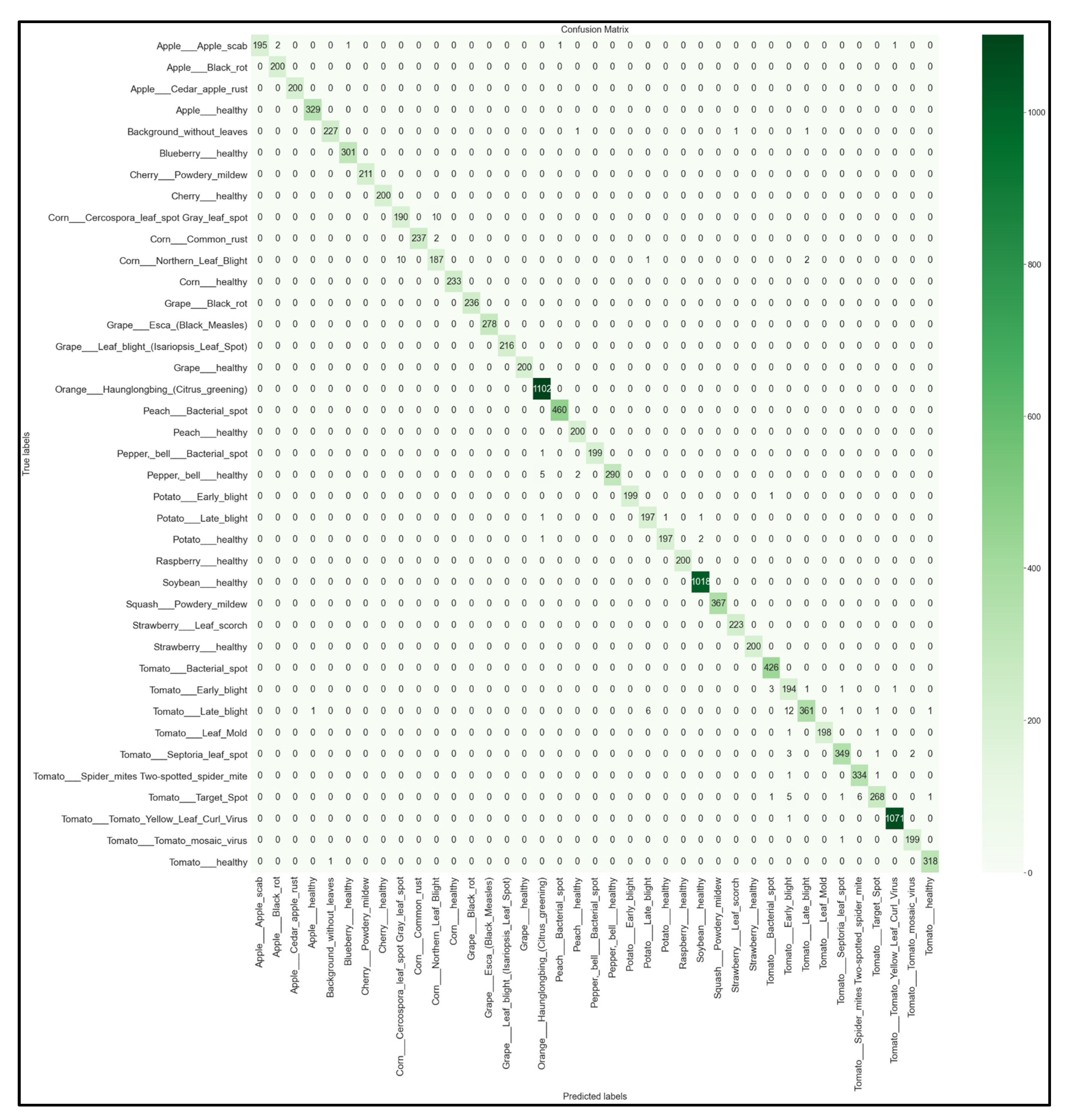
39 × 39 Confusion matrix for the NasNetMobile model with transfer learning Scenario 3 and the Proposed hyperparameters.
Figure 18.
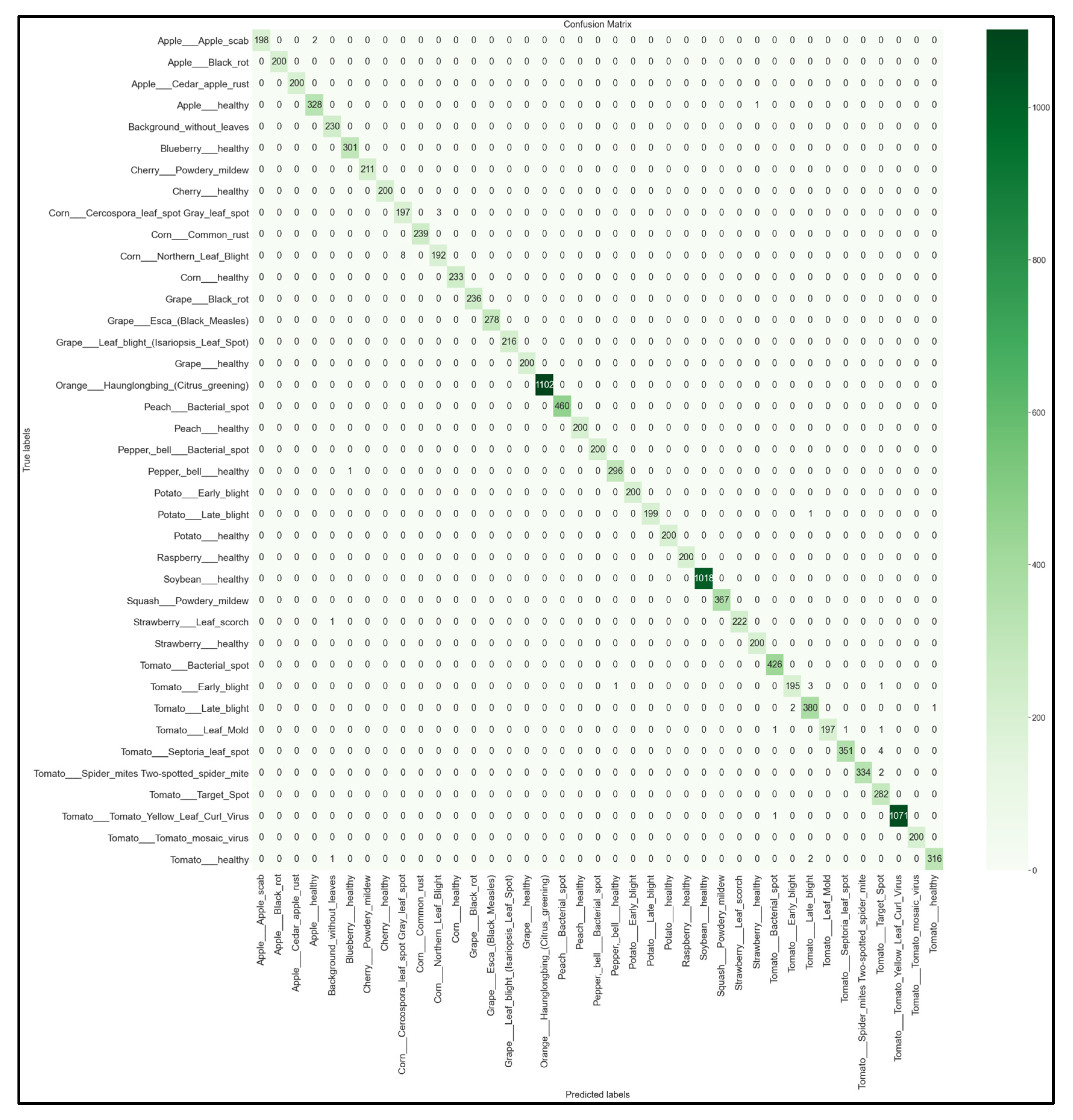
39 × 39 Confusion matrix for the MobileNet model with transfer learning Scenario 4 and the Proposed hyperparameters.
Figure 19.
39 × 39 Confusion matrix for the EfficientNetB0 model with transfer learning Scenario 4 and the Proposed hyperparameters.
Figure 20.
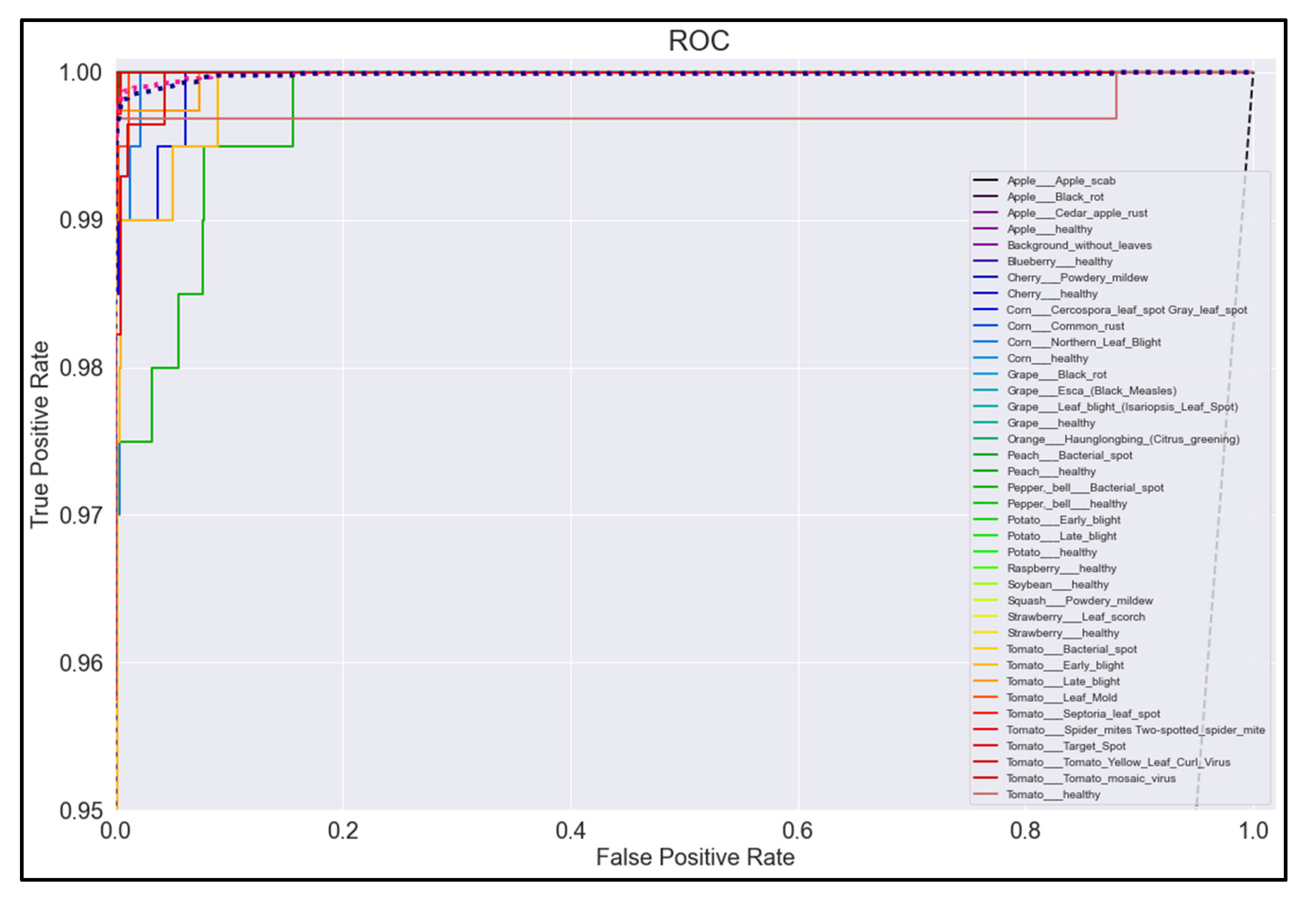
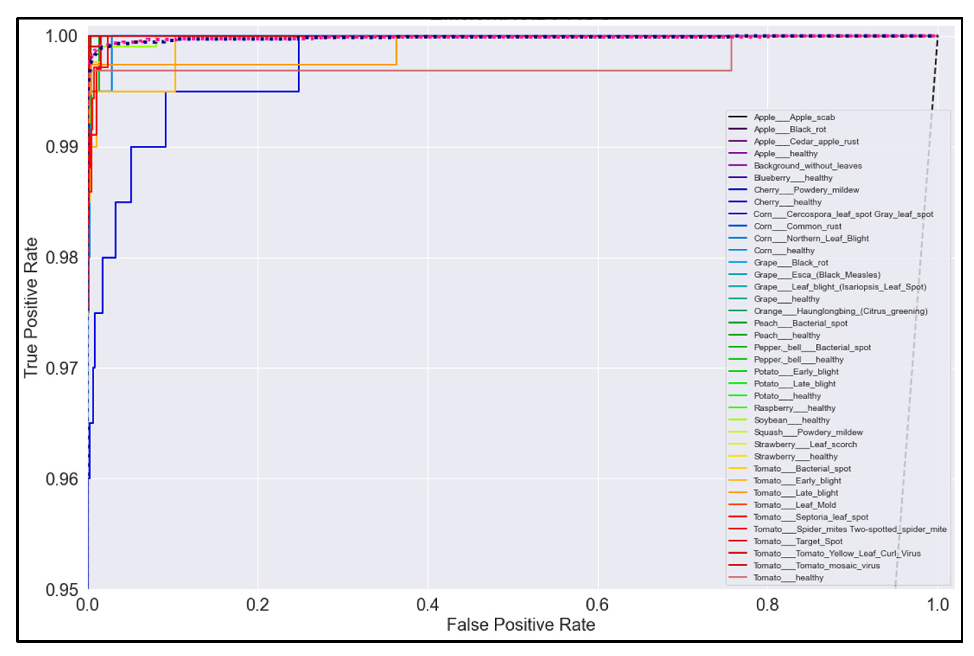
ROC Curve for MobileNetV2 model with transfer learning Scenario 3 and Proposed hyperparameters.
Figure 21.
ROC Curve for NasNetMobile model with transfer learning Scenario 3 and Proposed hyperparameters.
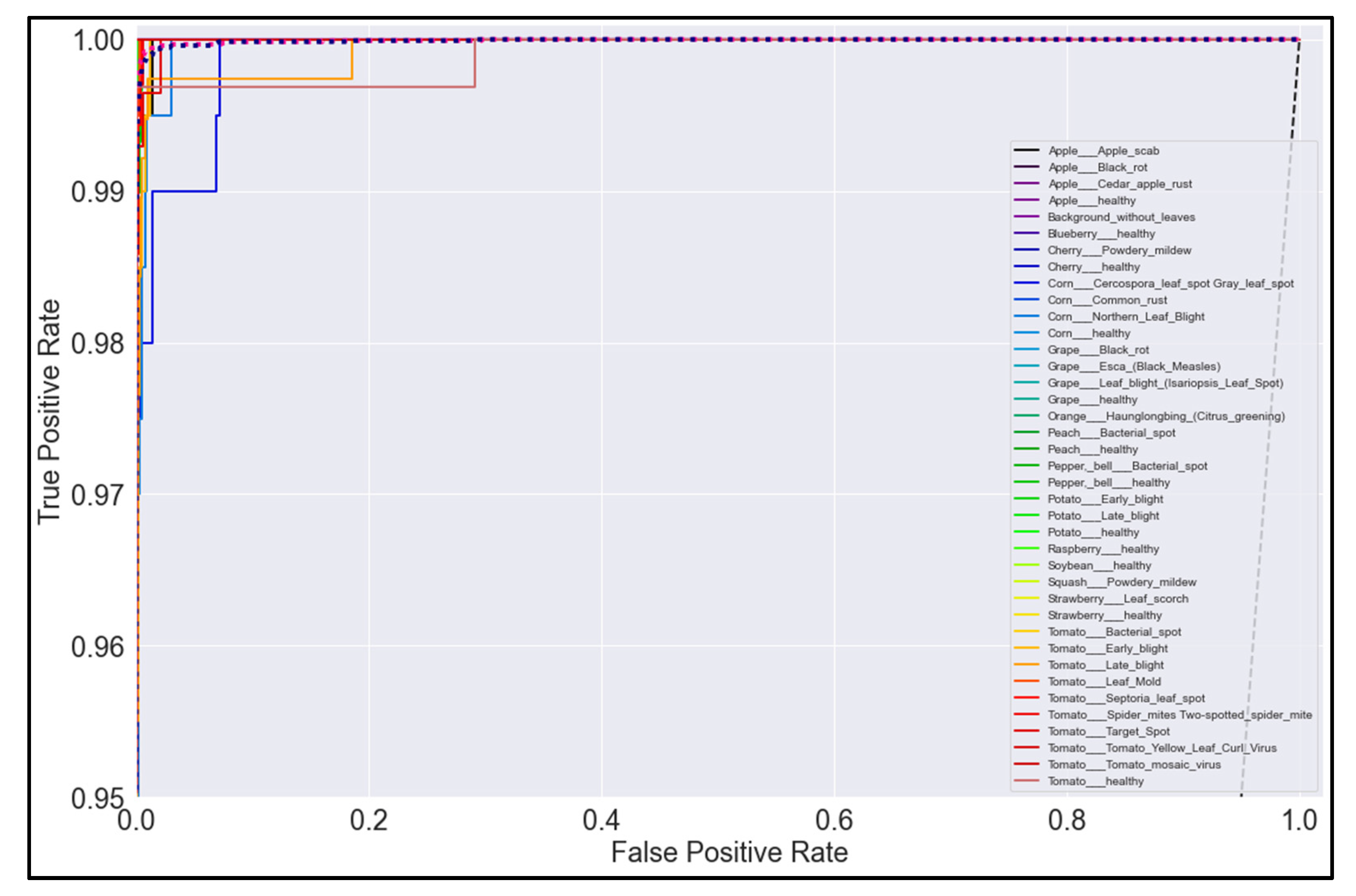
Figure 22.
ROC Curve for MobileNet model with transfer learning Scenario 4 and Proposed hyperparameters.
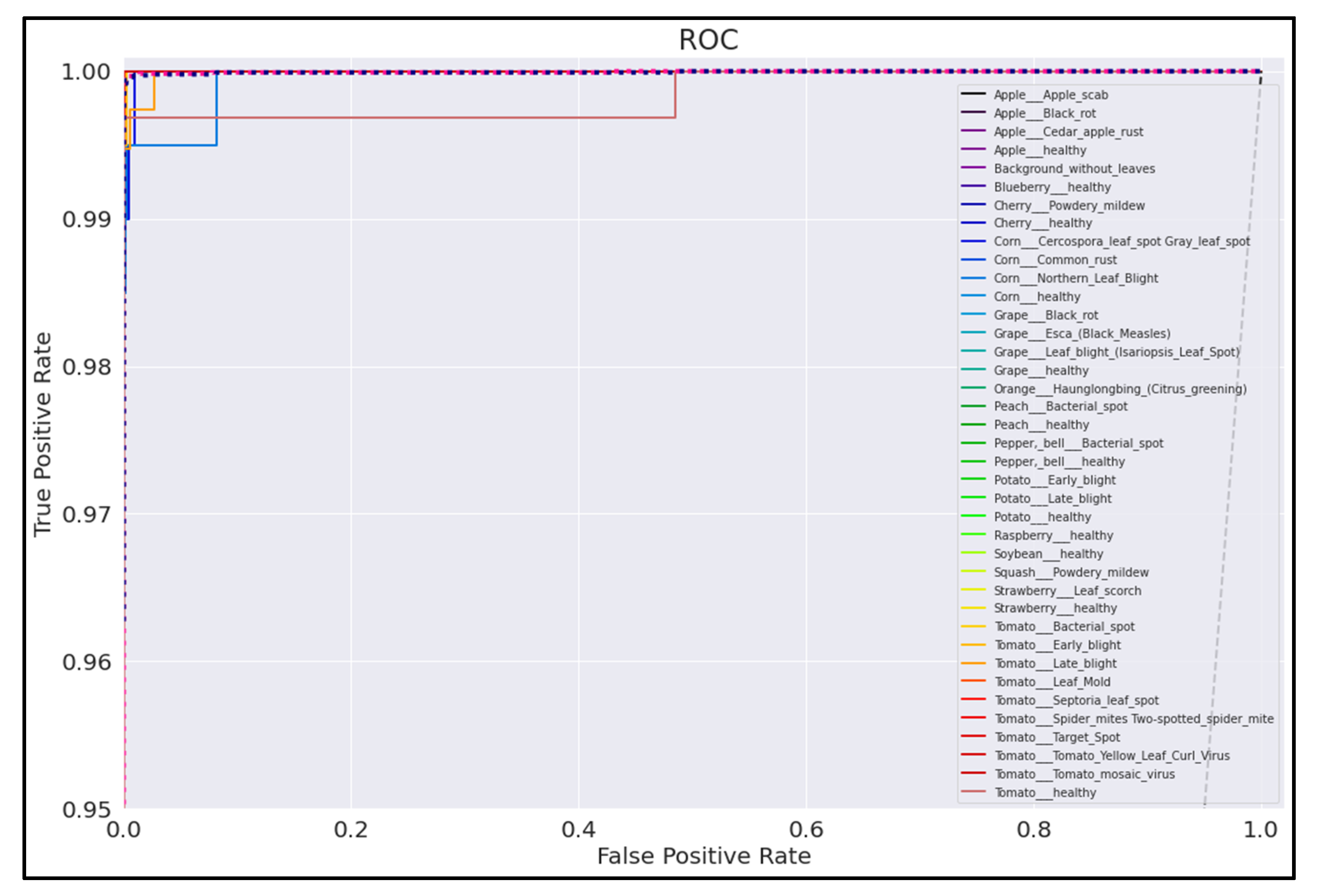
Figure 23.
ROC Curve for EfficientNetB0 model with transfer learning Scenario 4 and Proposed hyperparameters.
Figure 24.
(a) Precision vs Recall graph of 4-fold EfficientNetB0 model; (b) Histogram of F1-scores for 4-fold EfficientNetB0 model.
Figure 25.
(a) Home page of the mobile application; (b) Central activity of the mobile application displaying all of the system’s implemented functionalities.
Figure 26.
User-side walkthrough of the classification functionality of the system.
Figure 27.
Example of the process of viewing the plant care support information provided for a [species–disease] combination identified in a classification result.
Figure 28.
Viewing the list of all supported [species–disease] combinations and expanding the details of some of the species listed.
Figure 29.
Viewing a user’s classification history, with its minimizable “frequent classification” card, and an example of expanding the details of a history record.
Figure 30.
Configuring user settings (number of history records and location region).
Figure 31.
Example of generating user-wide spatiotemporal analytics for a selected region and season filter.
Figure 32.
Example of generating bar and pie charts to visualize the generated spatiotemporal analytics.
Figure 33.
Visualization of the Firestore database schema used for this project.
Table 1.
Evaluation scores for developed MobileNet models.
MobileNet Models
([Hyperparameter, Scenario] Variations) | Accuracy | Precision | Recall | F1-Score |
|---|
| Referenced Hyperparameters [19] | Sc. 1 | 0.41 | 0.54 | 0.46 | 0.43 |
| Sc. 2 | 0.69 | 0.77 | 0.69 | 0.68 |
| Sc. 3 | 0.82 | 0.85 | 0.82 | 0.82 |
| Sc. 4 | 0.82 | 0.85 | 0.82 | 0.83 |
| Proposed Hyperparameters | Sc. 1 | 0.99 | 0.99 | 0.99 | 0.99 |
| Sc. 2 | 0.99 | 0.99 | 0.99 | 0.99 |
| Sc. 3 | 0.99 | 0.99 | 0.99 | 0.99 |
| Sc. 4 | 0.99 | 0.99 | 0.99 | 0.99 |
Table 2.
Evaluation scores for developed MobileNetV2 models.
MobileNetV2 Models
([Hyperparameter, Scenario] Variations) | Accuracy | Precision | Recall | F1-Score |
|---|
| Referenced Hyperparameters [19] | Sc. 1 | 0.59 | 0.74 | 0.59 | 0.57 |
| Sc. 2 | 0.50 | 0.71 | 0.50 | 0.48 |
| Sc. 3 | 0.69 | 0.80 | 0.69 | 0.67 |
| Sc. 4 | 0.48 | 0.68 | 0.48 | 0.47 |
| Proposed Hyperparameters | Sc. 1 | 0.98 | 0.98 | 0.98 | 0.98 |
| Sc. 2 | 0.97 | 0.98 | 0.97 | 0.97 |
| Sc. 3 | 0.99 | 0.99 | 0.99 | 0.99 |
| Sc. 4 | 0.99 | 0.99 | 0.99 | 0.99 |
Table 3.
Evaluation scores for developed NasNetMobile models.
NasNetMobile Models
([Hyperparameter, Scenario] Variations) | Accuracy | Precision | Recall | F1-Score |
|---|
| Referenced Hyperparameters [19] | Sc. 1 | 0.82 | 0.87 | 0.82 | 0.81 |
| Sc. 2 | 0.88 | 0.92 | 0.88 | 0.88 |
| Sc. 3 | 0.72 | 0.79 | 0.72 | 0.70 |
| Sc. 4 | 0.17 | 0.38 | 0.17 | 0.15 |
| Proposed Hyperparameters | Sc. 1 | 0.98 | 0.98 | 0.98 | 0.98 |
| Sc. 2 | 0.98 | 0.98 | 0.98 | 0.98 |
| Sc. 3 | 0.99 | 0.99 | 0.99 | 0.99 |
| Sc. 4 | 0.99 | 0.99 | 0.99 | 0.99 |
Table 4.
Evaluation scores for developed EfficientNetB0 models.
EfficientNetB0 Models
([Hyperparameter, Scenario] Variations) | Accuracy | Precision | Recall | F1-Score |
|---|
| Referenced Hyperparameters [19] | Sc. 1 | 0.99 | 0.99 | 0.99 | 0.99 |
| Sc. 2 | 0.99 | 0.99 | 0.99 | 0.99 |
| Sc. 3 | 0.98 | 0.98 | 0.98 | 0.98 |
| Sc. 4 | 0.96 | 0.97 | 0.96 | 0.96 |
| Proposed Hyperparameters | Sc. 1 | 1.0 | 1.0 | 1.0 | 1.0 |
| Sc. 2 | 1.0 | 1.0 | 1.0 | 1.0 |
| Sc. 3 | 1.0 | 1.0 | 1.0 | 1.0 |
| Sc. 4 | 1.0 | 1.0 | 1.0 | 1.0 |
Table 5.
Mean Accuracy and F1-scores of best performing models of each network.
| Metric | MobileNetV2 | NasNetMobile | MobileNet | EfficientNet |
|---|
| Mean Accuracy | 0.77375 | 0.81625 | 0.8375 | 0.99 |
| Mean F1-Score | 0.765 | 0.81 | 0.84 | 0.99375 |
Table 6.
Example of a multi-class confusion matrix (4 × 4).
| Actual Class | Predicted Class |
|---|
| A. Apple Scab | B. Apple Black Rot | C. Apple Rust | D. Background |
|---|
| A. Apple Scab | TPApple Scab | BA | CA | DA |
| B. Apple Black Rot | AB | TPApple Black Rot | CB | DB |
| C. Apple Rust | AC | BC | TPApple Rust | DC |
| D. Background | AD | BD | CD | TPBackground |
Table 7.
EfficientNetB0 model: F1-scores per fold.
| Metrics | Fold 1 | Fold 2 | Fold 3 | Fold 4 |
|---|
| F1-Score | 0.99752332 | 0.99504282 | 0.99686251 | 0.9964706 |
| Mean F1-Score | 0.99647481438147 |
| Standard Deviation | 0.00090833778759 |
Table 8.
EfficientNetB0 model: Precision score per fold.
| Metrics | Fold 1 | Fold 2 | Fold 3 | Fold 4 |
|---|
| Precision | 0.9975028 | 0.99525983 | 0.99707548 | 0.99636672 |
| Mean Precision | 0.996551206305218 |
| Standard Deviation | 0.000848832773722 |
Table 9.
EfficientNetB0 model: Recall score per fold.
| Metrics | Fold 1 | Fold 2 | Fold 3 | Fold 4 |
|---|
| Recall | 0.99756669 | 0.9948848 | 0.99671894 | 0.99658669 |
| Mean Recall | 0.99643928335171 |
| Standard Deviation | 0.00097306173904 |
| Publisher’s Note: MDPI stays neutral with regard to jurisdictional claims in published maps and institutional affiliations. |
© 2022 by the authors. Licensee MDPI, Basel, Switzerland. This article is an open access article distributed under the terms and conditions of the Creative Commons Attribution (CC BY) license (https://creativecommons.org/licenses/by/4.0/).


