Model Distribution Effects on Likelihood Ratios in Fire Debris Analysis

Abstract
:
1. Introduction
2. Materials and Methods
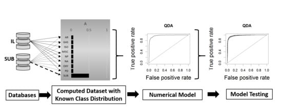
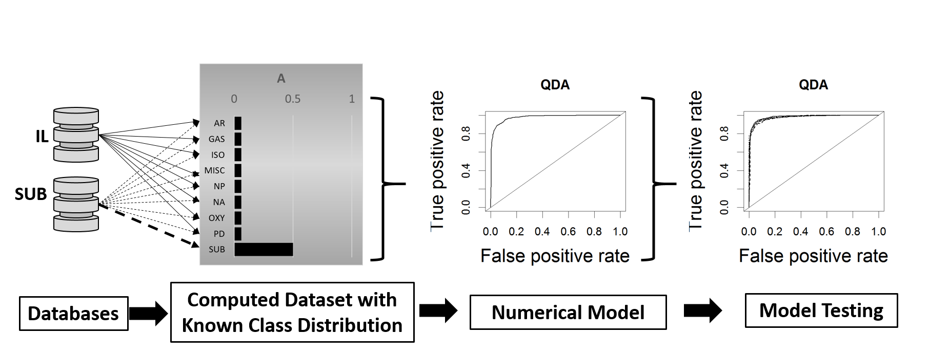
2.1. Computational Fire Debris Data Preparation
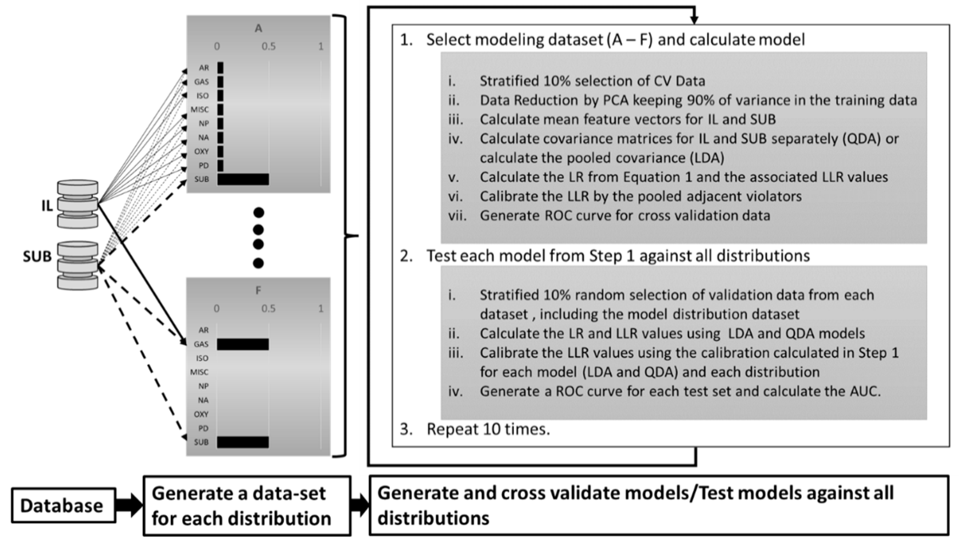
2.2. Model Development and Cross Validation
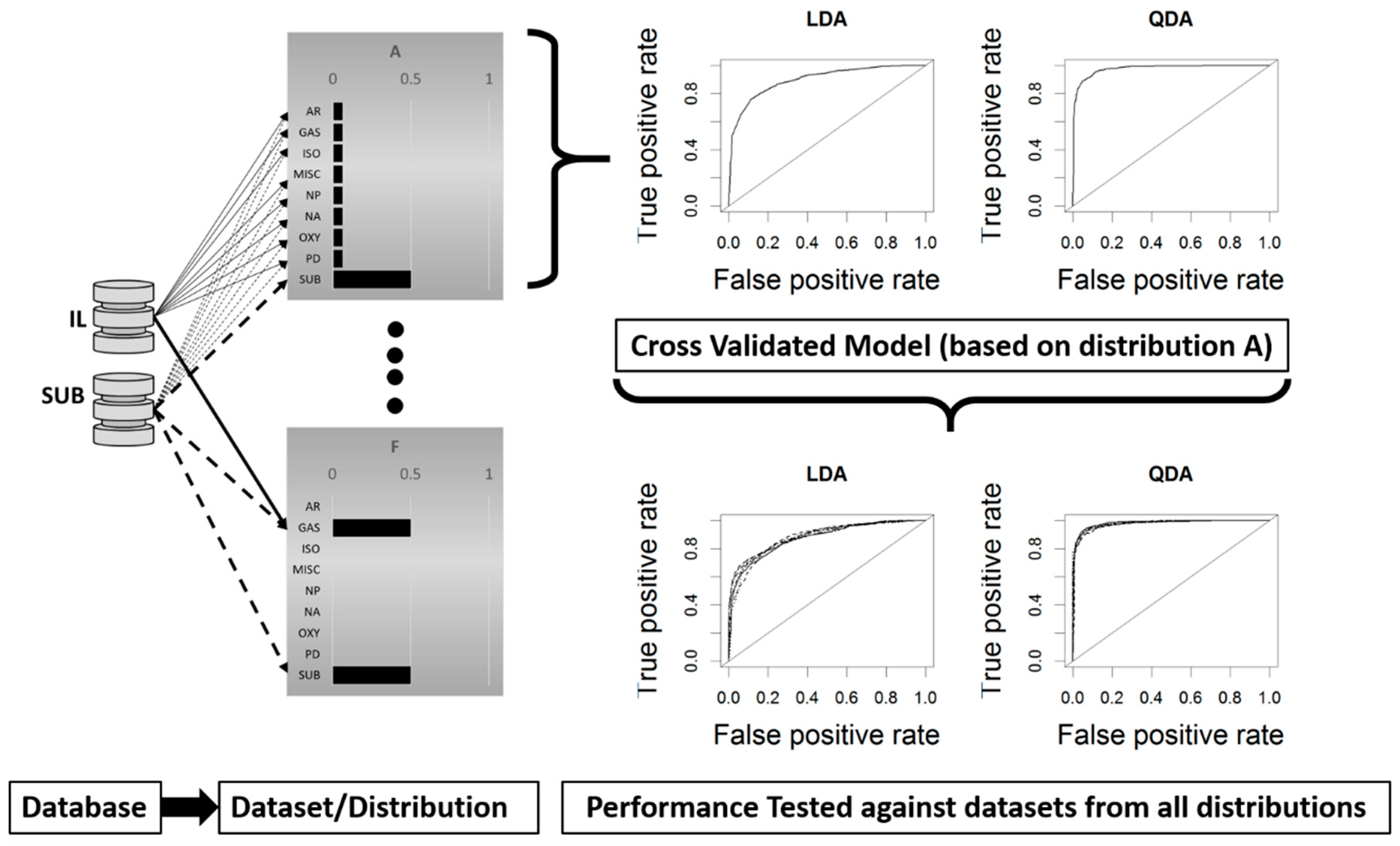
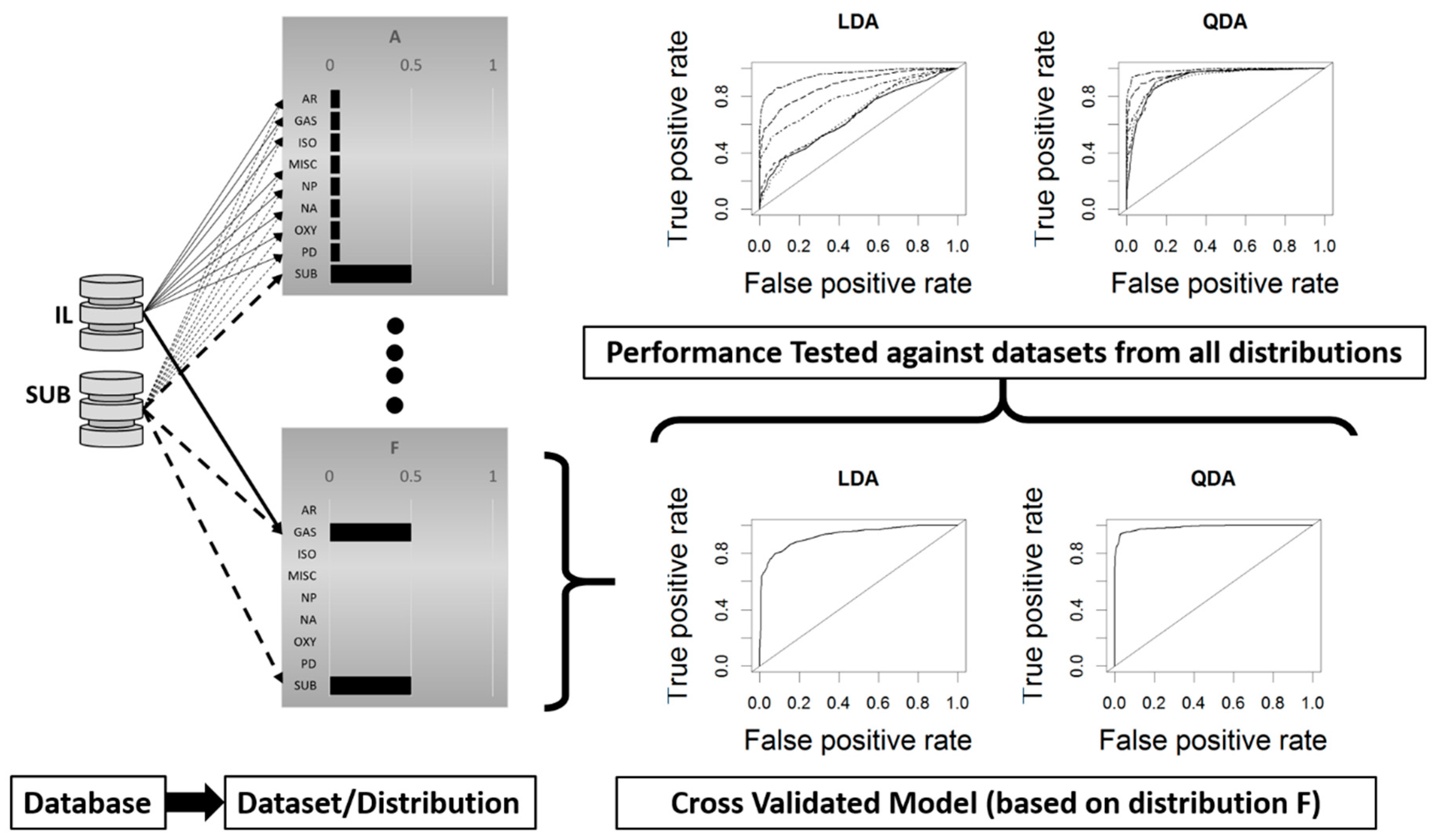
2.3. Model Testing Across Data Distributions
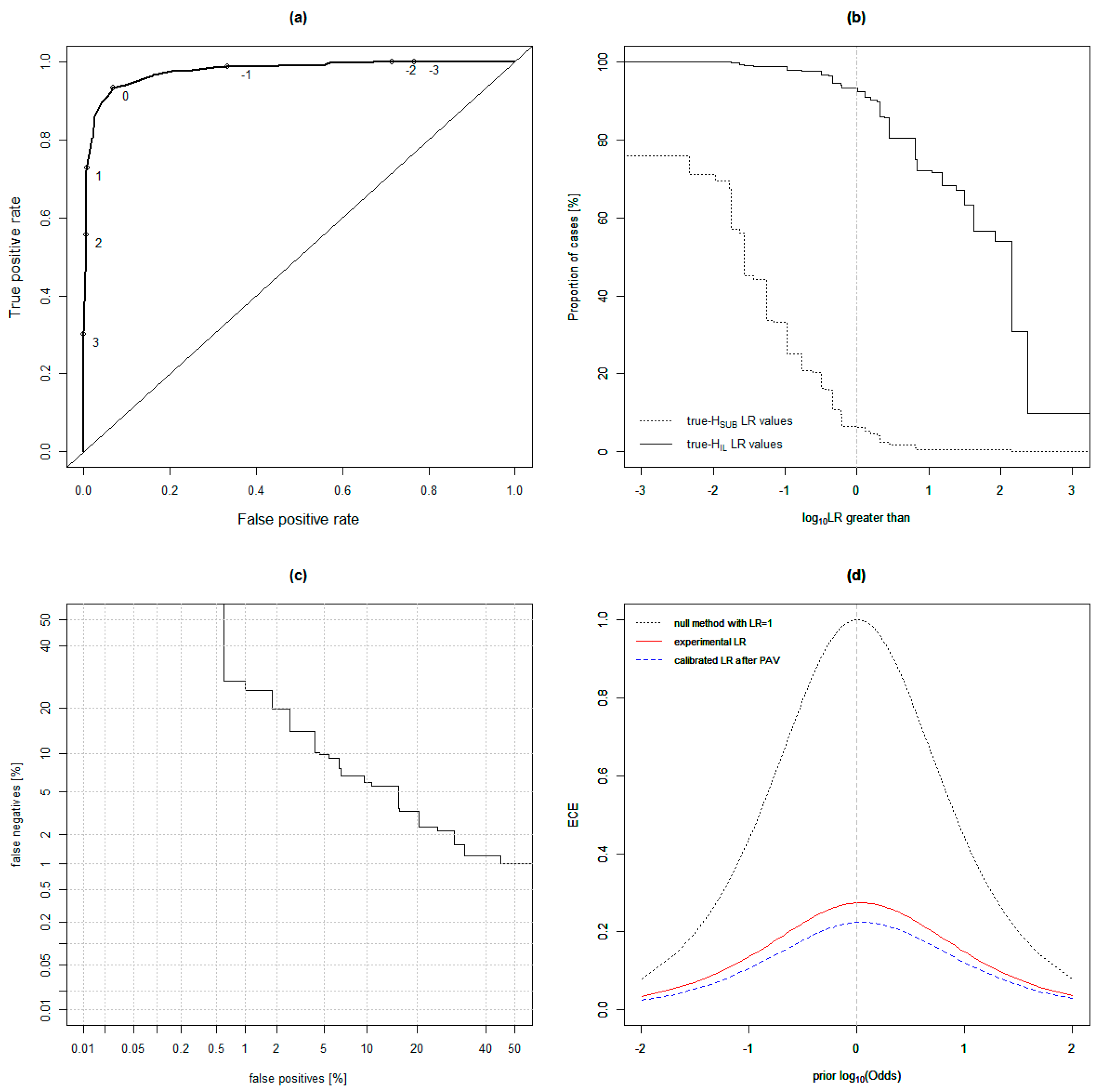
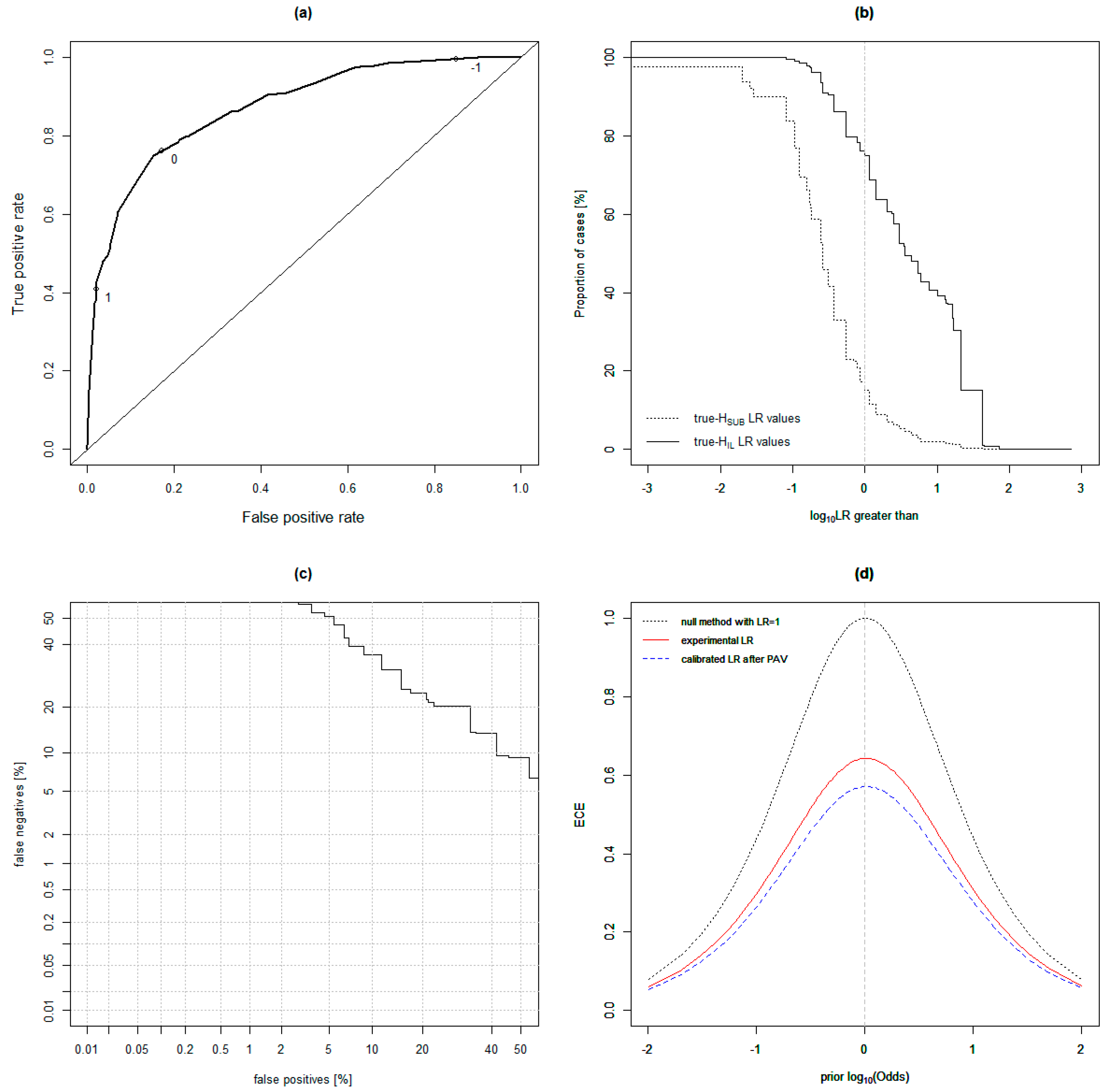
2.4. Model Testing Against Known Ground Truth-Simulated Casework Samples
3. Results
Cross Validation Testing Across Distributions
4. Discussion
4.1. Cross-Validation Testing Across Distributions
4.2. Model Comparisons
4.3. Testing the Quadratic Discriminant Analysis (QDA) Model on Known Ground Truth-Simulated Casework Samples
5. Conclusions
Author Contributions
Funding
Conflicts of Interest
References
- ASTM International. Standard Test Method for Ignitable Liquid Residues in Extracts from Fire Debris Samples by Gas Chromatography-Mass Spectrometry; ASTM International: West Conshohocken, PA, USA, 2014. [Google Scholar]
- Lopatka, M.; Sigman, M.E.; Sjerps, M.J.; Williams, M.R.; Vivo-Truyols, G. Class-conditional feature modeling for ignitable liquid classification with substantial substrate contribution in fire debris analysis. Forensic Sci. Int. 2015, 252, 177–186. [Google Scholar] [CrossRef] [PubMed]
- Sigman, M.E.; Williams, M.R. Assessing evidentiary value in fire debris analysis by chemometric and likelihood ratio approaches. Forensic Sci. Int. 2016, 264, 113–121. [Google Scholar] [CrossRef] [PubMed]
- Waddell, E.E.; Song, E.T.; Rinke, C.N.; Williams, M.R.; Sigman, M.E. Progress toward the determination of correct classification rates in fire debris analysis. J. Forensic Sci. 2013, 58, 887–896. [Google Scholar] [CrossRef] [PubMed]
- Waddell, E.E.; Williams, M.R.; Sigman, M.E. Progress toward the determination of correct classification rates in fire debris analysis ii: Utilizing soft independent modeling of class analogy (SIMCA). J. Forensic Sci. 2014, 59, 927–935. [Google Scholar] [CrossRef] [PubMed]
- Williams, M.R.; Sigman, M.E.; Lewis, J.; Pitan, K.M. Combined target factor analysis and bayesian soft-classification of interference-contaminated samples: Forensic fire debris analysis. Forensic Sci. Int. 2012, 222, 373–386. [Google Scholar] [CrossRef] [PubMed]
- Coulson, R.; Williams, M.R.; Allen, A.; Akmeemana, A.; Ni, L.; Sigman, M.E. Model-effects on likelihood ratios for fire debris analysis. Forensic Chem. 2018, 7, 38–46. [Google Scholar] [CrossRef]
- Zadora, G.; Neocleous, T. Likelihood ratio model for classification of forensic evidence. Analytica Chim. Acta 2009, 642, 266–278. [Google Scholar] [CrossRef] [PubMed]
- Zadora, G.; Martyna, A.; Ramos, D.; Aitken, C. Statistical Analysis in Forensic Science: Evidential Value of Multivariate Physicochemical Data; John Wiley & Sons Ltd.: West Sussex, UK, 2014. [Google Scholar]
- National Center for Forensic Science. Substrate Database, 2017 ed.; National Center for Forensic Science: Orlando, FL, USA, 2017. [Google Scholar]
- National Center for Forensic Science. Ignitable Liquids Reference Collection and Database (ILRC); National Center for Forensic Science: Orlando, FL, USA, 2017. [Google Scholar]
- Zadrozny, B.; Elkan, C. Transforming classifier scores into accurate multiclass probability estimates. In Proceedings of the Eighth ACM SIGKDD International Conference on Knowledge Discovery and Data Mining, Edmonton, AB, Canada, 23–25 July 2002; pp. 694–699. [Google Scholar]
- Sigman, M.E.; Williams, M.R.; Castelbuono, J.A.; Colca, J.G.; Clark, C.D. Ignitable liquid classification and identification using the summed-ion mass spectrum. Instrum. Sci. Technol. 2008, 36, 375–393. [Google Scholar] [CrossRef]
- De Leeuw, J.; Hornik, K.; Mair, P. Isotone optimization in R: Pool-adjacent-violators algorithm (PAVA) and active set methods. J. Stat. Softw. 2009, 32, 24. [Google Scholar] [CrossRef]
- Evett, I.W.; Jackson, G.; Lambert, J.A.; McCrossan, S. The impact of the principles of evidence interpretation on the structure and content of statements. Sci. Justice 2000, 40, 233–239. [Google Scholar] [CrossRef]


| Classes | A | B | C | D | E | F |
|---|---|---|---|---|---|---|
| Aromatic solvents (AR) | 0.063 | 0.094 | 0.042 | 0.044 | 0.005 | 0.000 |
| Gasoline (GAS) | 0.063 | 0.094 | 0.041 | 0.281 | 0.330 | 0.500 |
| Isoparaffinic solvents (ISO) | 0.063 | 0.094 | 0.062 | 0.054 | 0.003 | 0.000 |
| Miscellaneous (MISC) | 0.063 | 0.094 | 0.164 | 0.000 | 0.058 | 0.000 |
| Naphthenic paraffinic solvents (NP) | 0.063 | 0.094 | 0.030 | 0.034 | 0.002 | 0.000 |
| Normal alkanes (NA) | 0.063 | 0.094 | 0.028 | 0.039 | 0.003 | 0.000 |
| Oxygenates (OXY) | 0.063 | 0.094 | 0.123 | 0.034 | 0.012 | 0.000 |
| Petroleum distillates (PD) | 0.063 | 0.094 | 0.295 | 0.118 | 0.062 | 0.000 |
| Pyrolyzed substrates (SUB) | 0.500 | 0.250 | 0.215 | 0.394 | 0.525 | 0.500 |
| A | B | C | D | E | |
|---|---|---|---|---|---|
| B | 0.790 | ||||
| C | 0.719 | 0.800 | |||
| D | 0.793 | 0.780 | 0.717 | ||
| E | 0.771 | 0.706 | 0.661 | 0.846 | |
| F | 0.681 | 0.650 | 0.604 | 0.777 | 0.838 |
| Sample (Ground Truth) | Ignitable Liquid SRN/Class | Substrate Material Description | IL:SUB Ratio |
|---|---|---|---|
| A (SUB) | none | olefin carpet and padding | 0 |
| B (IL) | 120/isoparaffinic | leather jacket | 3.5 |
| C (IL) | 259/gasoline | vinyl flooring | 1 |
| D (SUB) | none | milk jug and duct tape | 0 |
| E (IL) | 46/MPD | roofing shingle | 1.76 |
| F (SUB) | none | vinyl flooring | 0 |
| G (SUB) | none | polyester carpet | 0 |
| H (IL) | 120/isoparaffinic | polyester carpet | 0.25 |
| I (IL) | 73/aromatic | olefin carpet and padding | 0.25 |
| J (SUB) | none | laminate flooring and newspaper | 0 |
| K (IL) | 73/aromatic | polyester carpet and padding | 1 |
| L (SUB) | none | polyester carpet and padding | 0 |
| M (SUB) | none | leather jacket | 0 |
| N (IL) | 259/gasoline | milk jug and duct tape | 0.25 |
| O (IL) | 46/MPD | laminate flooring and newspaper | 1 |
| P (SUB) | none | roofing shingle | 0 |
| Testing Distributions in Columns | ||||||
|---|---|---|---|---|---|---|
| Model | A | B | C | D | E | F |
| IL and SUB Independent Covariance Matrices (QDA) | ||||||
| A | 0.975 ± 0.005 | 0.975 ± 0.004 | 0.972 ± 0.004 | 0.976 ± 0.003 | 0.975 ± 0.004 | 0.978 ± 0.004 |
| B | 0.927 ± 0.008 | 0.941 ± 0.005 | 0.923 ± 0.008 | 0.937 ± 0.006 | 0.935 ± 0.006 | 0.942 ± 0.008 |
| C | 0.921 ± 0.007 | 0.929 ± 0.007 | 0.928 ± 0.007 | 0.929 ± 0.006 | 0.928 ± 0.007 | 0.930 ± 0.009 |
| D | 0.954 ± 0.006 | 0.956 ± 0.005 | 0.949 ± 0.004 | 0.974 ± 0.003 | 0.965 ± 0.006 | 0.976 ± 0.003 |
| E | 0.969 ± 0.008 | 0.969 ± 0.004 | 0.966 ± 0.003 | 0.977 ± 0.004 | 0.982 ± 0.003 | 0.984 ± 0.003 |
| F | 0.923 ± 0.012 | 0.921 ± 0.009 | 0.924 ± 0.007 | 0.951 ± 0.008 | 0.962 ± 0.006 | 0.985 ± 0.003 |
| Pooled Covariance Matrix for IL and SUB (LDA) | ||||||
| A | 0.878 ± 0.008 | 0.876 ± 0.011 | 0.875 ± 0.011 | 0.884 ± 0.008 | 0.879 ± 0.012 | 0.882 ± 0.010 |
| B | 0.873 ± 0.008 | 0.877 ± 0.012 | 0.870 ± 0.014 | 0.879 ± 0.007 | 0.878 ± 0.010 | 0.881 ± 0.010 |
| C | 0.865 ± 0.008 | 0.866 ± 0.013 | 0.875 ± 0.014 | 0.868 ± 0.008 | 0.865 ± 0.011 | 0.863 ± 0.012 |
| D | 0.864 ± 0.010 | 0.859 ± 0.009 | 0.853 ± 0.013 | 0.898 ± 0.008 | 0.889 ± 0.013 | 0.913 ± 0.011 |
| E | 0.855 ± 0.010 | 0.852 ± 0.011 | 0.858 ± 0.014 | 0.892 ± 0.010 | 0.910 ± 0.012 | 0.928 ± 0.009 |
| F | 0.665 ± 0.021 | 0.664 ± 0.015 | 0.691 ± 0.016 | 0.777 ± 0.017 | 0.864 ± 0.013 | 0.943 ± 0.011 |
| Sample | Ground Truth | LLR | Hypothesis Supported | Level of Support | Misleading Evidence | IL:SUB Ratio |
|---|---|---|---|---|---|---|
| A | SUB | 0.292 | HIL | Limited | Yes | 0 |
| B | IL | −1.037 | HSUB | Moderate | Yes | 3.5 |
| C | IL | 2.577 | HIL | Moderately Strong | No | 1 |
| D | SUB | −0.508 | HSUB | Limited | No | 0 |
| E | IL | 2.095 | HIL | Moderately Strong | No | 1.76 |
| F | SUB | −0.508 | HSUB | Limited | No | 0 |
| G | SUB | 0.000 | HSUB | Limited | No | 0 |
| H | IL | 0.249 | HIL | Limited | No | 0.25 |
| I | IL | 20.000 | HIL | Very Strong | No | 0.25 |
| J | SUB | −0.508 | HSUB | Limited | No | 0 |
| K | IL | 20.000 | HIL | Very Strong | No | 1 |
| L | SUB | −0.348 | HSUB | Limited | No | 0 |
| M | SUB | −1.037 | HSUB | Moderate | No | 0 |
| N | IL | 2.577 | HIL | Moderately Strong | No | 0.25 |
| O | IL | 0.292 | HIL | Limited | No | 1 |
| P | SUB | 0.292 | HIL | Limited | Yes | 0 |
© 2018 by the authors. Licensee MDPI, Basel, Switzerland. This article is an open access article distributed under the terms and conditions of the Creative Commons Attribution (CC BY) license (http://creativecommons.org/licenses/by/4.0/).
Share and Cite
Allen, A.; Williams, M.R.; Thurn, N.A.; Sigman, M.E. Model Distribution Effects on Likelihood Ratios in Fire Debris Analysis. Separations 2018, 5, 44. https://doi.org/10.3390/separations5030044
Allen A, Williams MR, Thurn NA, Sigman ME. Model Distribution Effects on Likelihood Ratios in Fire Debris Analysis. Separations. 2018; 5(3):44. https://doi.org/10.3390/separations5030044
Chicago/Turabian StyleAllen, Alyssa, Mary R. Williams, Nicholas A. Thurn, and Michael E. Sigman. 2018. "Model Distribution Effects on Likelihood Ratios in Fire Debris Analysis" Separations 5, no. 3: 44. https://doi.org/10.3390/separations5030044
APA StyleAllen, A., Williams, M. R., Thurn, N. A., & Sigman, M. E. (2018). Model Distribution Effects on Likelihood Ratios in Fire Debris Analysis. Separations, 5(3), 44. https://doi.org/10.3390/separations5030044