Abstract
Current standard approaches for quantitation of volatile organic compounds (VOCs) in outdoor air are labor-intensive and/or require additional equipment. Solid-phase microextraction (SPME) is a simpler alternative; however, its application is often limited by complex calibration, the need for highly pure gases and the lack of automation. Earlier, we proposed the simple, automated and accurate method for quantitation of benzene, toluene, ethylbenzene and xylenes (BTEX) in air using 20 mL headspace vials and standard addition calibration. The aim of present study was to expand this method for quantitation of >20 VOCs in air. Twenty-five VOCs were chosen for the method development. Polydimethylsiloxane/divinylbenzene (PDMS/DVB) fiber provided better combination of detection limits and relative standard deviations of calibration slopes than other studied fibers. Optimal extraction time was 10 min. For quantification of all analytes except n-undecane, crimp top vials with samples should not stand on the autosampler tray for >8 h, while 22 most stable analytes can be quantified during 24 h. The developed method was successfully tested for automated quantification of VOCs in outdoor air samples collected in Almaty, Kazakhstan. Relative standard deviations (RSDs) of the responses of 23 VOCs were below 15.6%. Toluene-to-benzene concentration ratios were below 1.0 in colder days, indicating that most BTEX originated from non-transport-related sources.
1. Introduction
The pollution of ambient and indoor air are the main sources of risk to human health in the world [1]. Air pollution leads to destruction of ecosystems and creates huge economic and social damages to society. There is a direct relationship between a level of air pollution and risk in the development of cancer, cardiovascular, respiratory and other diseases [1]. The most difficult and important process in quantification of chemical pollutants in ambient air is sampling. Sampling must be representative taking into account physicochemical properties of analytes and their concentrations in air [2].
Current standard sampling approaches for quantification of VOCs in air [2,3,4] are mainly based on collecting air samples into evacuated canisters [2,5] or trapping analytes onto sorbent tubes [3,6] followed by the analysis on a gas chromatograph (GC) with a chosen detector, mostly being flame-ionization (FID) or mass spectrometry (MS). Despite good reliability, these sampling techniques [4] are quite complex, labor- and time-consuming, as well as requiring additional equipment. Air sampling by standard methods based, e.g., on sorbent tubes [2,3], requires additional equipment such as an air sampling pump and a thermal desorption system connected to a gas chromatograph. Before air sampling, it is necessary to thoroughly clean sorbent tubes from possible contaminants and residues from previous sampling by highly pure helium. In order to solve these problems, it is necessary to reduce the volume of organic solvents used for extraction, or completely exclude them; fully or partially automate the sampling process; integrate the sampling and measurement stages; and reduce laboratory work and time costs. Additional problems may include carryover of analytes and clogging of the cryogenic focusing system [7], which considerably limit the application of standard methods. Therefore, low-cost, simple and solvent-free methods for quantification of VOCs in the air combining sampling and sample preparation in one step are needed. Solid-phase microextraction (SPME) that is based on extraction of VOCs by a micro coating, followed by desorption in a GC injection port, meets these requirements [8]. SPME is widely used for the determination of VOCs in ambient air (Table 1), indoor air and different emissions [9,10,11,12,13,14,15,16,17,18]. Methods based on SPME do not need a pump and a thermal desorption system. Desorption of analytes is fast resulting in narrow peaks of analytes without a cryogenic focusing.

Table 1.
Methods for quantification of organic compounds in ambient air by exposed solid-phase microextraction (SPME) fibers.
Despite the high efficiency of the described methods for determination of VOCs in air by SPME (Table 1), there are still challenges limiting their application in routine and research environmental laboratories. Some authors report limitations due to labor-intensive calibration, i.e., requirements for construction of gas generation system with a known concentration of analytes [19,21,24,26]. Most methods require using high-purity gases for preparation of calibration samples, which can be difficult to purchase and prepare. Baimatova et al. [25] developed a very simple, automated and accurate method for quantification of BTEX using SPME and successfully applied it for the analysis of ambient air in Almaty, Kazakhstan. Sampling was conducted with 20 mL crimp top vials, which were transported to the laboratory, located on the Combi PAL (CTC Analytics, Switzerland) autosampler tray and automatically analyzed using GC-MS. To simplify the method, the authors used standard addition calibration, which did not require any additional equipment and pure gases. The only major drawback of this method was that it allowed quantification of only four analytes [25], while more than 100 organic compounds are present in outdoor air of Almaty [27]. Lee et al. [24] developed the method for determination of 36 VOCs. However, the sampling was done into Tedlar bags, which did not allow automation. In addition, the calibration was carried out with a standard gas mixture of VOCs in pure nitrogen.
The objective of this study was to improve the method developed by Baimatova et al. [25] for quantitation of >20 VOCs in 20 mL ambient air samples using SPME and GC-MS. During this study, SPME fiber, extraction, desorption and storage times were optimized. The developed method was applied for quantification of chosen VOCs in outdoor air of Almaty, Kazakhstan.
2. Materials and Methods
2.1. Chemicals
Analytes of interest were chosen according to the literature review of VOCs determination in ambient air in different cities [28,29,30,31,32,33] and previous studies of compounds detected in the exhausts of six arbitrarily chosen cars of different models and production years [27]. Chosen analytes belong to several classes of pollutants having various physicochemical properties (Table S1 in Supplementary Materials). All solutions were prepared in methanol (purity ≥ 99.9%) that was obtained from Sigma-Aldrich (St. Louis, MO, USA). Helium (purity > 99.995%) was obtained from “Orenburg-Tehgas” (Orenburg, Russia).
2.2. GC-MS Conditions
All analyses were conducted on a 7890A/5975C Triple-Axis Detector diffusion pump-based GC-MS (Agilent, Wilmington, DE, USA) equipped with a split/splitless inlet and MPS2 (Gerstel, Mülheim an der Ruhr, Germany) autosampler capable of automated SPME. The inlet was equipped with a 0.75 mm ID SPME liner (Supelco, Bellefonte, PA, USA) and operated in splitless mode. For separation, a 60 m × 0.25 mm DB-WAXetr (Agilent, Santa Clara, CA, USA) column with a film thickness of 0.50 µm was used at the constant flow of He (1.0 mL min−1). Oven temperature was programmed from initial 35 °C (held for 5 min) to 150 °C (held for 5 min) at the heating rate of 10 °C min−1, then to 250 °C (held for 7 min) at the heating rate of 10 °C min−1. Total GC run time of the analysis was 38.5 min. The MS detector worked in selected ion monitoring (SIM) mode. All ions were divided into six consequently detected groups for better shape of peaks and lower limits of detection (Table 2). An example of a chromatogram is shown in Figure S1 in Supplementary Materials. Peaks were identified using retention times of each analyte, which were preliminarily determined by analyzing standard solutions of pure analytes and confirmed in full scan (m z−1 10–250 amu) mode of the MS detector. Optimal dwell time for each ion was 50–100 ms. The temperatures of MS interface, ion source and quadrupole were 250, 230 and 150 °C, respectively.
Table 2.
MS detection program of analytes in SIM mode.
2.3. Selection of the Optimal SPME Fiber
Standard addition calibration plots were obtained for all 25 analytes using the four most common commercially available SPME fibers: 85 µm Carboxen(Car)/polydimethylsiloxane(PDMS), 100 µm PDMS, 65 µm PDMS/divinylbenzene(DVB) and 50/30 µm DVB/Car/PDMS (all–from Supelco, Bellefonte, PA, USA). The calibration process was the same as described by Baimatova et al. [25]. Calibration samples were prepared by adding 1.00 µL of a standard solution of analytes (0.50, 1.00, 2.00 and 4.00 ng µL−1 for benzene, toluene and alkanes; and 0.050, 0.100, 0.200 and 0.400 ng µL−1 for other analytes) into the 20 mL crimp-top headspace vial (HTA, Brescia, Italy) filled with laboratory air. Ranges of concentrations of VOCs added to calibration samples were chosen in order to cover their real concentrations in ambient air (according to the preliminary screening results). Added concentrations of benzene, toluene, and alkanes in the calibration samples were 25, 50, 100 and 200 µg m−3. Added concentrations of ethylbenzene, m-, p-, o-xylenes, polycyclic aromatic hydrocarbons and other analytes were 2.5, 5, 10 and 20 µg m−3. Extraction was conducted at room temperature (22 °C) for 10 min; desorption time was 1 min.
From the calibration plots, relative standard deviations (RSDs) of slopes and limits of detection (LODs) were determined. RSDs of slopes were determined using the LINEST function of Microsoft Excel software (Microsoft® Excel for Office 365, Version 1909, Redmond, WA, USA). LODs were calculated using:
where b is the intercept of a calibration plot; a is the slope of a calibration plot; Cadd is the standard addition concentration (µg m−3); and S/N is the signal-to-noise ratio.
2.4. Effects of Extraction and Desorption Times
The experiment was conducted on air samples with standard additions of all analytes at 100 µg m−3. The following extraction times were studied: 1, 3, 5, 7, 10, 20 and 30 min followed by a 5 min desorption. Desorption times 1, 3, 5, 7 and 10 min were studied after 10 min extraction of analytes.
2.5. Effect of Storage Time
Effects of storage time on the responses of analytes were studied in crimped 20 mL vials with concentrations of standard additions of analytes at 100 µg m−3. Samples were stored at room temperature (22 °C) on the autosampler tray during 0, 2, 4, 8, 16, 24, 36 and 48 h, and extracted by 65 µm PDMS/DVB fiber for 10 min followed by a 1 min desorption. Two replicate samples were analyzed after each storage time. Significance of differences (p-value) between the initial response of analytes and its response after a certain storage time was estimated using a two-sample two-tailed Student’s t-test with a preset relative standard deviation (10%).
2.6. Estimation of the Method Accuracy
Accuracy of the method was estimated using spike recoveries from laboratory air samples. Concentrations of analytes in laboratory air were determined using a standard addition calibration by dividing intercepts by slopes. Three replicate laboratory air samples, which were collected at the same time as samples used for preparing calibration standards, were spiked at C = 100 µg m−3 for benzene, toluene and alkanes, and at C = 10.0 µg m−3 for other analytes. After analysis, spike recoveries (R, %) were determined using
where Cmeas is the determined concentration of an analyte in a spiked sample (µg m−3); Cair is the concentration of an analyte in the laboratory air (µg m−3); and Csp is the concentration of the standard addition of an analyte (µg m−3).
2.7. Air Sampling and Analysis
The developed method was applied for monitoring of VOCs in ambient air in Almaty on 30 March, 2 April and 4 April 2019. The sampling process and coordinates of sampling locations (Table S2 in Supplementary Materials) were identical to those used by Baimatova et al. in 2015 [25].
Prior to sampling, all 20 mL vials and septa were washed using distilled water and conditioned at 160 °C for 4 h. Ambient air samples were collected into 20 mL crimp vials (i.e., by opening the vial to air and shaking for ~60 sec) and then sealed with aluminum caps and PTFE-silicone septa (Agilent, Santa Clara, CA, USA). Vials were transported to the laboratory in 1 L clean glass jars to prevent possible losses of analytes during the transportation. Vials with air samples were placed on the autosampler tray. Air samples were extracted from the vial using 65 µm PDMS/DVB fiber coating at optimized method parameters. Calibration plots were obtained before each sampling day. Weather conditions, such as temperature, humidity, wind velocity and pressure, were taken from the public database Gismeteo (Table S3 in Supplementary Materials).
3. Results
3.1. Selection of the Optimal SPME Fiber
Selection of the optimal SPME fiber for quantification of multiple analytes having different physicochemical properties is a difficult process. In most cases, the fibers are chosen based on an experimental or theoretical basis. Experimental fiber selection is straightforward only when one fiber provides greater responses for all analytes. In other cases, a theoretical approach can be involved based on known selectivity of the coatings to compounds having different molecular weights and polarities [34]. In our study, the selection of the optimal fiber was conducted based on the two most important indicators: limit of detection (LOD) and relative standard deviation (RSD) of a calibration slope. Lower LODs will allow greater applicability of the method, while lower RSDs would provide better accuracy and precision. We estimated how many analytes can be determined at different LODs and RSDs. After determining LOD and RSD for each analyte using the four most common commercial fibers (Car/PDMS, PDMS, DVB/Car/PDMS and PDMS/DVB), it was checked how many analytes have LODs below 1, 2, 5 and 10 µg m−3, and RSDs below 1%, 2%, 5% and 10% using each fiber.
LODs ≤ 1 µg m−3 for the greatest number of analytes (20 of 25) were achieved using the DVB/Car/PDMS fiber (Table 3). Car/PDMS and PDMS/DVB fibers provided such LODs only for 17 analytes. LODs ≤ 2 µg m−3 were achieved for 23 analytes using DVB/Car/PDMS and PDMS/DVB fibers. Such LOD using these fibers was not achieved only for n-hexane and n-hexadecane. LODs ≤ 5 µg m−3 were achieved for 24 analytes using PDMS/DVB fiber. LODs ≤ 10 µg m−3 were achieved for all 25 analytes using PDMS, DVB/Car/PDMS and PDMS/DVB fibers. Overall, DVB/Car/PDMS and PDMS/DVB fibers provide greatest numbers of analytes at most target LODs. At the same time, PDMS/DVB provides lower LODs for three PAHs, which are considered more toxic compared to other analytes.
Table 3.
Limits of detection obtained using different SPME fibers.
When comparing RSDs of calibration slopes (Table 4), PDMS/DVB fiber also provides better values. RSDs are below 5% for 17 analytes and below 10%—for 22 analytes, which is greater than for DVB/Car/PDMS fiber—11 and 20 analytes, respectively. When using PDMS/DVB fiber, RSDs of slopes above 10% were obtained only for methyl ethyl ketone (25%), 1,2-dichloroethane (20%) and p-xylene (15%). When using DVB/Car/PDMS fiber, RSDs of slopes for benzaldehyde and n-hexadecane were 79% and 32%, respectively. Thus, based on these results, PDMS/DVB fiber was chosen as most appropriate for simultaneous quantification of 25 VOCs.
Table 4.
Relative standard deviations of calibration slopes obtained using different SPME fibers.
3.2. Effects of Extraction and Desorption Times
Extraction and desorption times are important parameters of VOC quantification by SPME, which have an impact on intensity of analyte responses. Speed of equilibration during the extraction stage depends on a vessel volume, the diffusion coefficient of an analyte and its distribution constant between the coating and the air [35]. The equilibrium between the fiber and air for almost all analytes was reached after 5–10 min of extraction (Figure 1). Extraction time did not affect the responses of methylene chloride, methyl ethyl ketone and 1,2-dichloroethane—their responses varied by 1–13%. The responses for benzene were stabilized after 3 min of extraction. Based on the obtained results, an extraction time of 10 min was chosen as optimal.
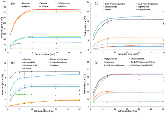
Figure 1.
Effect of extraction time on responses of analytes: (a)—benzene, toluene, ethylbenzene, m,p,o-xylenes; (b)—2,2,4-trimethylpentane, benzaldehyde, phenol, 1,3,5-trimethylbenzene, naphthalene, acenaphthene; (c)—n-heptane, n-decane, n-undecane, fluorene, methyl ethyl ketone, 1,2-dichloroethane, 3-picoline, and (d)—propylbenzene, n-hexadecane, 1,2,4-trimethylbenzene, chlorobenzene, 1,1,2,2-tetrachloroethylene, methylene chloride.
The increase in desorption time above 1 min had no significant effects on responses of all studied VOCs (Figure S2 in Supplementary Materials). After this time, the responses varied by 0.43–15%. Therefore, the desorption time of 1 min was chosen as the optimal.
3.3. Effect of Storage Time
During transportation and storage of air samples, concentrations of analytes can decrease due to their decomposition, losses via leaks and adsorption to internal walls of a vial and septum. The approach proposed by Baimatova et al. [25] was used to minimize the losses of analytes. The goal of this experiment was to estimate losses of analytes during their storage on the autosampler tray.
Figure 2 shows the effect of storage time on responses of analytes. Two-sample two-tailed t-tests indicated that the changes in responses of n-undecane, acenaphthene and fluorene in relation to initial values were significant (p < 0.05 at RSD = 10%) after 24 h of storage (Table S4 in Supplementary Materials), while responses of other 22 analytes were stable. After 48 h of storage, changes in responses of n-undecane, n-hexadecane, acenaphthene and fluorene were significant. Greater losses of more hydrophobic analytes could be explained by their adsorption to a hydrophobic surface of a PTFE-lined septum being in direct contact with air. Despite these septa being considered highly inert, adsorption of very hydrophobic compounds by PTFE was earlier reported in the literature [36]. For achieving the greatest accuracy for these analytes, samples should be analyzed as quickly as possible, e.g., during the first 8 h after sampling.
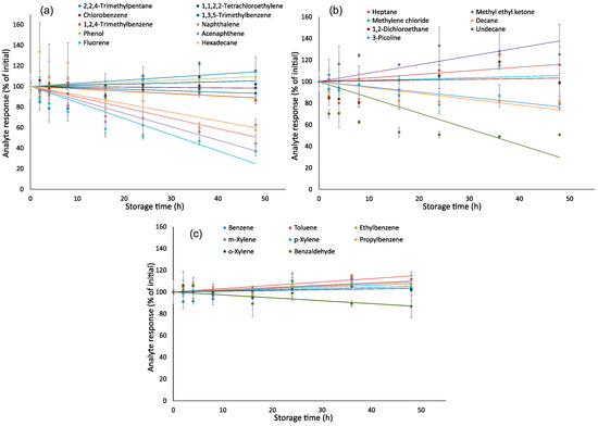
Figure 2.
Effect of storage time on responses of analytes: (a)—2,2,4-trimethylpentane, chlorobenzene, 1,2,4-trimethylbenzene, phenol, fluorene, 1,1,2,2-tetrachloroethylene, 1,3,5-trimethylbenzene, naphthalene, acenaphthene, hexadecane; (b)—n-heptane, methylene chloride, 1,2-dichloroethane, 3-picoline, methyl ethyl ketone, n-decane, n-undecane, and (c)—benzene, toluene, ethylbenzene, m,p,o-xylenes, propylbenzene, benzaldehyde.
3.4. Estimation of the Method Accuracy
Spike recoveries of all analytes except methyl ethyl ketone, methylene chloride, 3-picoline and n-hexadecane were 90–105% (Table 5), which is consistent with the results of previous experiments. Lower recoveries of methyl ethyl ketone, methylene chloride, 3-picoline and n-hexadecane could be explained by high RSDs in their determined concentrations, which were 7.4%, 17%, 43% and 11%, respectively. RSDs of other analytes were 1.8–6.5%.
Table 5.
Spike recoveries of analytes.
3.5. Air Sampling and Analysis
During the monitoring of the atmospheric air in Almaty using the optimized method, all analytes were detected except methyl ethyl ketone and 1,2-dichloroethane. Mean concentrations of analytes ranged from 0.2 to 83, from 0.1 to 70 and from 0.1 to 74 µg m−3 on 30 March, 2 April and 4 April, respectively. The highest concentrations (0.7–89 µg m−3) for 16 of the 23 analytes were detected on the 3rd day of sampling (Table 6). It can be caused by higher temperatures (14–16 °C) than on previous sampling days (6–11 °C). The highest concentrations for the rest of the VOCs, such as benzene, propylbenzene, benzaldehyde and hexadecane, were detected on March 30, which made up 56, 0.3, 1.8 and 123 µg m−3, respectively. The 2nd sampling day showed the highest concentrations of naphthalene, phenol and fluorene—2.4, 3.9 and 0.8 µg m−3, respectively. The lowest concentrations of the greatest number of analytes (16) were detected in sampling point P2 (Table S5 in Supplementary Materials) located in the upper part of the city close to mountains. The highest concentrations of the greatest number of analytes (12) were detected in sampling point P3 located in the central part of the city.
Table 6.
Measured VOC concentrations in air.
The relative standard deviations of three replicate analyses of the air samples did not exceed 15.6%. From 108 measurements, the greatest numbers of outliers (one out of three replicate measurements according to Grubbs’ test) were identified for n-hexadecane (19), methylene chloride (14), n-undecane (13) and acenaphthene (12). No outliers were identified for ethylbenzene and m-xylene.
Toluene-to-benzene (T/B) concentration ratios during the sampling period varied from 0.46 to 1.69. During the first two days of sampling, T/B ratios were below 1 indicating that the main source of BTEX was not transport. During these two days, the temperatures were 3–7 °C lower than during the third day of sampling, and the central and domestic heating systems were more active. During the third day of sampling, T/B ratios were 1.69 and 1.06, and the main BTEX emissions originated from transport. The same trend was reported for the similar period in 2015 [25]. However, T/B were lower than 1 mostly in days with negative temperatures. In 2019, such ratios were observed at temperatures between 6 and 11 °C, which could mean that the fraction of BTEX emissions from transport-related sources decreased since 2015.
4. Conclusions
A low-cost method for quantitation of multiple VOCs in ambient air using SPME-GC-MS was developed. It was proven that 65 µm PDMS/DVB fiber provides a better combination of detection limits, accuracy and precision compared to 85 µm Car/PDMS, 100 µm PDMS and 50/30 µm DVB/Car/PDMS. The increase in extraction time above 10 min did not have a significant impact on the responses of analytes. Optimal desorption time is 1 min. For quantification of all analytes, except undecane, vials with samples should not stand on the autosampler tray for more than 8 h. Quantification of 22 of the most stable analytes can be conducted during 24 h after sampling. Spike recoveries of 21 of the 25 chosen analytes were 90–105%. Recoveries of other analytes were 51–89% at RSDs of 7.4–43%.
The developed method was successfully applied for quantification of chosen analytes in atmospheric air of Almaty in Spring, 2019. On average, the completely automated analysis of one sample took 50–60 min, which was enough to analyze 24 (18 air + 6 calibration) air samples per day. All analytes were detected, except methyl ethyl ketone and 1,2-dichloroethane. RSDs of the responses of 23 VOCs varied from 0.1% to 15.6%. The use of three replicate samples allowed identifying outliers. For 18 detected analytes, the fraction of outliers was <18%. Results for the other five detected analytes contained 10–20% outliers. Mean concentrations of 23 VOCs during all sampling times ranged from 0.1 to 83 µg m−3. Toluene-to-benzene concentrations ratios were below 1.0 in colder days of sampling, indicating that most BTEX in these days originated from non-transport-related sources. The obtained results prove that the method is very simple, automated, low-cost and provides sufficiently low detection limits, which allow recommending it for monitoring of a wide range of VOCs in atmospheric air of Almaty and other similar cities. The measured concentrations cannot be used to generalize the air pollution problem in Almaty because additional research is needed for this purpose. These data along with the developed method can be useful for improving the air pollution monitoring program in Almaty.
Supplementary Materials
The following are available online at https://www.mdpi.com/2297-8739/6/4/51/s1, Figure S1: Chromatogram obtained using the developed method based on SPME-GC-MS of air sample with Cadd = 100 µg m−3, Figure S2: Effect of desorption time on responses of analytes, Table S1: The list of chosen VOCs and its physical properties, Table S2: Coordinates of sampling locations, Table S3: Weather conditions on sampling days, Table S4: Probabilities of difference between initial responses of analytes and their responses after different storage times, Table S5: Sampling locations where lowest and highest concentrations of analytes were determined at different sampling times.
Author Contributions
Conceptualization, B.K. and N.B.; methodology, O.P.I. and N.B.; validation, O.P.I., N.B. and B.K.; formal analysis, O.P.I., N.B. and B.K.; investigation, O.P.I. and N.B.; writing—original draft preparation, O.P.I. and N.B.; writing—review and editing, B.K.; visualization, O.P.I., N.B. and B.K.; supervision, B.K.; project administration, N.B.; funding acquisition, B.K.
Funding
This research was funded by the Ministry of Education and Science of the Republic of Kazakhstan, grant number AP05133158.
Acknowledgments
The authors would like to thank Al-Farabi Kazakh National University for the postdoctoral scholarship of Nassiba Baimatova, and a Ph.D. student of Al-Farabi Kazakh National University, Bauyrzhan Bukenov, for technical support during this study.
Conflicts of Interest
The authors declare no conflict of interest.
References
- World Health Organization. Ambient Air Pollution: A Global Assessment of Exposure and Burden of Disease; WHO: Geneva, Switzerland, 2016. [Google Scholar]
- US EPA. Compendium Method TO-14A Determination of Volatile Organic Compounds (VOCs) in Ambient Air Using Specially Prepared Canisters with Subsequent Analysis by Gas Chromatography; United States Environmental Protection Agency: Cincinnati, OH, USA, 1999.
- US EPA. Compendium Method TO-17 Determination of Volatile Organic Compounds in Ambient Air Using Active Sampling Onto Sorbent Tubes; United States Environmental Protection Agency: Cincinnati, OH, USA, 1999.
- Król, S.; Zabiegała, B.; Namieśnik, J. Monitoring VOCs in atmospheric air II. Sample collection and preparation. Trends Anal. Chem. 2010, 29, 1101–1112. [Google Scholar] [CrossRef]
- Miller, L.; Xu, X. Multi-season, multi-year concentrations and correlations amongst the BTEX group of VOCs in an urbanized industrial city. Atmos. Environ. 2012, 61, 305–315. [Google Scholar] [CrossRef]
- Goodman, N.B.; Steinemann, A.; Wheeler, A.J.; Paevere, P.J.; Cheng, M.; Brown, S.K. Volatile organic compounds within indoor environments in Australia. Build. Environ. 2017, 122, 116–125. [Google Scholar] [CrossRef]
- Woolfenden, E. Monitoring VOCs in air using sorbent tubes followed by thermal desorption-capillary GC analysis: Summary of data and practical guidelines. J. Air Waste Manag. Assoc. 1997, 47, 20–36. [Google Scholar] [CrossRef]
- Pawliszyn, J. (Ed.) Applications of Solid Phase Microextraction. In RSC Chromatography Monographs; Royal Society of Chemistry: Cambridge, UK, 1999; ISBN 978-0-85404-525-9. [Google Scholar]
- Haberhauer-Troyer, C.; Rosenberg, E.; Grasserbauer, M. Evaluation of solid-phase microextraction for sampling of volatile organic sulfur compounds in air for subsequent gas chromatographic analysis with atomic emission detection. J. Chromatogr. A 1999, 848, 305–315. [Google Scholar] [CrossRef]
- Tuduri, L.; Desauziers, V.; Fanlo, J.L. Dynamic versus static sampling for the quantitative analysis of volatile organic compounds in air with polydimethylsiloxane-Carboxen solid-phase microextraction fibers. J. Chromatogr. A 2002, 963, 49–56. [Google Scholar] [CrossRef]
- Ouyang, G. 8-SPME and Environmental Analysis. In Handbook of Solid Phase Microextraction; Elsevier Inc.: Amsterdam, The Netherlands, 2012; pp. 251–290. [Google Scholar] [CrossRef]
- Tumbiolo, S.; Gal, J.-F.; Maria, P.-C.; Zerbinati, O. Determination of benzene, toluene, ethylbenzene and xylenes in air by solid phase micro-extraction/gas chromatography/mass spectrometry. Anal. Bioanal. Chem. 2004, 380, 824–830. [Google Scholar] [CrossRef] [PubMed]
- Prikryl, P.; Sevcik, J.G.K. Characterization of sorption mechanisms of solid-phase microextraction with volatile organic compounds in air samples using a linear solvation energy relationship approach. J. Chromatogr. A 2008, 1179, 24–32. [Google Scholar] [CrossRef]
- Yassaa, N.; Meklati, B.Y.; Cecinato, A. Analysis of volatile organic compounds in the ambient air of Algiers by gas chromatography with a b-cyclodextrin capillary column. J. Chromatogr. A 1999, 846, 287–293. [Google Scholar] [CrossRef]
- Tumbiolo, S.; Gal, J.-F.; Maria, P.; Zerbinati, O. SPME sampling of BTEX before GC/MS analysis: Examples of outdoor and indoor air quality measurements in public and private sites. Ann. Chim. 2005, 95, 757–766. [Google Scholar] [CrossRef]
- Koziel, J.A.; Pawliszyn, J. Air sampling and analysis of volatile organic compounds with solid phase microextraction. J. Air Waste Manag. Assoc. 2001, 51, 173–184. [Google Scholar] [CrossRef] [PubMed]
- Curran, K.; Underhill, M.; Gibson, L.T.; Strlic, M. The development of a SPME-GC/MS method for the analysis of VOC emissions from historic plastic and rubber materials. Microchem. J. 2016, 124, 909–918. [Google Scholar] [CrossRef]
- Luca, A.; Kjær, A.; Edelenbos, M. Volatile organic compounds as markers of quality changes during the storage of wild rocket. Food Chem. 2017, 232, 579–586. [Google Scholar] [CrossRef]
- Parshintsev, J.; Niina, K.; Hartonen, K.; Miguel, L.; Jussila, M.; Kajos, M.; Kulmala, M.; Riekkola, M. Field measurements of biogenic volatile organic compounds in the atmosphere by dynamic solid-phase microextraction and portable gas chromatography-mass spectrometry. Atmos. Environ. 2015, 115, 214–222. [Google Scholar]
- Zain, S.M.S.M.; Shaharudin, R.; Kamaluddin, M.A.; Daud, S.F. Determination of hydrogen cyanide in residential ambient air using SPME coupled with GC–MS. Atmos. Pollut. Res. 2017, 8, 678–685. [Google Scholar] [CrossRef]
- Mokbel, H.; Al Dine, E.J.; Elmoll, A.; Liaud, C.; Millet, M. Simultaneous analysis of organochlorine pesticides and polychlorinated biphenyls in air samples by using accelerated solvent extraction (ASE) and solid-phase micro-extraction (SPME) coupled to gas chromatography dual electron capture detection. Environ. Sci. Pollut. Res. 2016, 23, 8053–8063. [Google Scholar] [CrossRef]
- Naccarato, A.; Tassone, A.; Moretti, S.; Elliani, R.; Sprovieri, F.; Pirrone, N.; Tagarelli, A. A green approach for organophosphate ester determination in airborne particulate matter: Microwave-assisted extraction using hydroalcoholic mixture coupled with solid-phase microextraction gas chromatography-tandem mass spectrometry. Talanta 2018, 189, 657–665. [Google Scholar] [CrossRef]
- Hussam, A.; Alauddin, M.; Khan, A.H.; Chowdhury, D.; Bibi, H.; Bhattacharjee, M.; Sultana, S. Solid phase microextraction: Measurement of volatile organic compounds (VOCs) in Dhaka city air pollution. J. Environ. Sci. Health Part A 2002, 37, 1223–1239. [Google Scholar] [CrossRef]
- Lee, J.H.; Hwang, S.M.; Lee, D.W.; Heo, G.S. Determination of volatile organic compounds (VOCs) using tedlar bag/solid-phase microextraction/gas chromatography/mass spectrometry (SPME/GC/MS) in ambient and workplace air. Bull. Korean Chem. Soc. 2002, 23, 488–496. [Google Scholar]
- Baimatova, N.; Kenessov, B.; Koziel, J.A.; Carlsen, L.; Bektassov, M.; Demyanenko, O.P. Simple and accurate quantification of BTEX in ambient air by SPME and GC-MS. Talanta 2016, 154, 46–52. [Google Scholar] [CrossRef]
- Woolcock, P.J.; Koziel, J.A.; Johnston, P.A.; Brown, R.C.; Broer, K.M. Analysis of trace contaminants in hot gas streams using time-weighted average solid-phase microextraction: Pilot-scale validation. Fuel 2015, 153, 552–558. [Google Scholar] [CrossRef]
- Carlsen, L.; Baimatova, N.; Kenessov, B.; Kenessova, O. Assessment of the air quality of Almaty. Focussing on the traffic component. Int. J. Biol. Chem. 2013, 5, 49–69. [Google Scholar]
- Nicoara, S.; Tonidandel, L.; Traldi, P.; Watson, J.; Morgan, G.; Popa, O. Determining the levels of volatile organic pollutants in urban air using a gas chromatography-mass spectrometry method. J. Environ. Public Health 2009, 2009, 148527. [Google Scholar] [CrossRef] [PubMed]
- Lee, S.C.; Chiu, M.Y. Volatile organic compounds (VOCs) in urban atmosphere of Hong Kong. Chemosphere 2002, 48, 375–382. [Google Scholar] [CrossRef]
- Khan, A.; Szulejko, J.E.; Kim, K.H.; Brown, R.J.C. Airborne volatile aromatic hydrocarbons at an urban monitoring station in Korea from 2013 to 2015. J. Environ. Manag. 2018, 209, 525–538. [Google Scholar] [CrossRef] [PubMed]
- Li, L.; Li, H.; Zhang, X.; Wang, L.; Xu, L.; Wang, X.; Yu, Y.; Zhang, Y.; Cao, G. Pollution characteristics and health risk assessment of benzene homologues in ambient air in the northeastern urban area of Beijing, China. J. Environ. Sci. 2014, 26, 214–223. [Google Scholar] [CrossRef]
- Zhang, Y.; Mu, Y. Atmospheric BTEX and carbonyls during summer seasons of 2008–2010 in Beijing. Atmos. Environ. 2012, 59, 186–191. [Google Scholar] [CrossRef]
- Bigazzi, A.Y.; Figliozzi, M.A.; Luo, W.; Pankow, J.F. Breath Biomarkers to Measure Uptake of Volatile Organic Compounds by Bicyclists. Environ. Sci. Technol. 2016, 50, 5357–5363. [Google Scholar] [CrossRef]
- Pawliszyn, J. Handbook of Solid Phase Microextraction; Elsevier Inc.: Amsterdam, The Netherlands, 2012; ISBN 9780124160170. [Google Scholar]
- Kenessov, B.; Derbissalin, M.; Koziel, J.A.; Kosyakov, D.S. Modeling solid-phase microextraction of volatile organic compounds by porous coatings using finite element analysis. Anal. Chim. Acta 2019, 1076, 73–81. [Google Scholar] [CrossRef]
- Lion, L.W. Sorption and Transport of Polynuclear Aromatic Hydrocarbons in Low-Carbon Aquifer Materials; AFESC: Ithaca, NY, USA, 1988. [Google Scholar]


© 2019 by the authors. Licensee MDPI, Basel, Switzerland. This article is an open access article distributed under the terms and conditions of the Creative Commons Attribution (CC BY) license (http://creativecommons.org/licenses/by/4.0/).