The Nonlinear Dynamic Behavior of a Particle on a Vibrating Screen Based on the Elastoplastic Contact Model

Abstract

The dynamic response of particles is closely related to screening efficiency. To study the dynamic response of particles, the dynamic equations of a particle on a screening surface are established based on the elastoplastic contact model of spherical particles and are solved for the coal particle. Then, the trajectories of the particles are given with different falling heights and particle radii. The completely different trajectories with slight changes in the falling height and particle radius indicate strong nonlinearity. Second, the nonlinear dynamic behavior under different amplitudes and frequencies is discussed, and the route of transition from quasiperiodic motion to chaotic motion is revealed. Finally, we discuss the average speed along the screening surface considering the frequency, amplitude, friction coefficient, inclination angle, and vibration direction angle. In addition, the convergence conditions of particle motion are proposed, and they are only affected by the inclination angle and friction angle. The results show that in the normal direction of the vibrating screen, the particle motion is quasiperiodic at low frequencies. With increasing frequency, the motion of the particle becomes chaotic, and its Poincaré map becomes petal-shaped. In addition, the number of petals increases at the mutation of the bifurcation diagram. The increase in frequency, amplitude and inclination angle and the decrease in friction coefficient lead to an increase in particle speed along the screen surface. In addition, the particle speed reaches a maximum when the vibration direction angle is 65°. This work provides a theoretical basis for controlling the thickness of granular material flow on a vibrating screen and selecting screening process parameters.

1. Introduction

High particle efficiency is the most important problem for vibrating screens [1]. The present studies for the screening theory of granular materials mainly focus on simulating the screening process by using the discrete element method (DEM) [2], the screening experiment for choosing optimal vibrating parameters (amplitude, frequency, inclination angle, etc.) [3], the trajectory of particles bouncing on a vibrating screen and the invention of new types of vibrating screens [4]. The ultimate purpose is to improve screen efficiency.

The essence of screening is to apply a small amplitude and suitable vibrational frequency to make the particles bounce and filter smaller particles under the screen [5]. Therefore, the key problem of the screening process is the dynamic behavior of the particles on the vibrating screen. DEM, as an effective numerical simulation technique, is a powerful method for predicting the motion and statement of the particles in the screening process [6,7]. DEM can obtain the key parameters, which include screening, particle speed, mass distribution, and impact force. The screening mechanism is revealed more easily with the help of DEM simulations. EDEM (the world’s first multi-purpose DEM modeling software, which can be used to simulate and analyze the production process of particle processing and manufacturing equipment in industrial production), the most commonly used simulation software for DEM, is a reliable method for simulating the screening processing of vibrating screening.

However, the dynamic behavior of the particles in EDEM software does not strictly obey the law of Hertz’s contact model and Thornton’s elastoplastic contact model. The coefficient of restitution in EDEM is set as a constant, which ignores the nonlinearity of the contact model despite the calculation of the contact force being based on Hertz’s model because of the large number of particles. Furthermore, the calculation of the contact force is not important for the screening process. In addition, the nonlinear dynamic behavior of particles on the screen surface reflects the screening process under different screening parameters and granular materials, and it is of great significance for revealing the screening mechanism.

The experimental method is a powerful way to study the screening mechanism as well, and it mainly focuses on screening granular materials to measure the content on and under the screen to calculate the screening efficiency. Meanwhile, the screening parameters are optimized by repeatedly changing the vibration parameters. Jiang [8] used a disequilibrium excitation vibrating screen to screen moist coal to improve the screening efficiency by changing the vibrating parameters. The physical screening method is absolutely accurate, but it is labor-intensive and time-consuming. The adjustable parameters are limited by the equipment. Additional equipment, including a high-speed camera and three-component acceleration sensors, should be set when extra parameters, such as particle speed and vibrating trajectory, are needed. In addition, the small particles are difficult to monitor by using a high-speed camera because the particle flow covers the small particles in the screening process.

Therefore, the behavior of particles on the screening surface is addressed by using a theoretical method. Wang [9] discussed one particle’s dynamic behavior on a nonsimple harmonic vibrating screen, and the particle speed in different areas of the vibrating screen was given. However, the contact model between the vibrating screen and particles was linear.

In the field of vibration screening, little research considers the nonlinear contact model between vibrating screens and granular materials. Yang [10] discussed the vibroimpact response of the particle elastic impact on a metal plate without vibration based on Hertz’s contact model. Dong [11] discussed the dynamic behavior of a vibrating plate at high frequency by extracting the particle load based on a linear contact model.

The nonlinear contact model is the fundamental reason for the nonlinear motion of particles on a vibrating screen. In 1896, Hertz [12] derived the elastic contact model between two spheres. The force–displacement relationship (FDR) is given by

$$F=\frac{4}{3}E\sqrt{R}{\delta }^{1.5}$$

(1)

where E is Young’s modulus, R is the radii of particles, δ is relative deformation.

Hurt and Crossley [13] proposed the viscoelastic contact model of two spheres based on Hertz’s theory, and the FDR is shown as follows:

$$F=K{\delta }^n+\chi {\delta }^n\dot{\delta }$$

(2)

where K is stiffness coefficient, χ is damping coefficient, n is the coefficient of contact according to the contact type.

In 1997, Thornton [14] found that energy loss caused by elastoplastic deformation is the main reason for different coefficients of restitution between different spheres. The collision process can be divided into three periods, including the elastic compression period, elastoplastic compression period, and elastic recovery period, and the FDR is given by:

$$F=\pi {\delta }_{y}R(\delta -{\delta }_y)+\frac{4}{3}E\sqrt{R}{\delta }_y^{1.5}$$

(3)

$$F=\frac{4}{3}E\sqrt{R}{\left(\delta -{\delta }_y\right)}^{1.5}$$

(4)

where δ_y is the ultimate deformation in the elastic contact period.

Many researchers have focused on the theoretical model of particle contact based on the above theory [15,16,17,18,19,20,21,22,23]. Essentially, there are few differences between these calculations with different models [24]. Meanwhile, the validity of the theoretical models is difficult to prove because of the lack of experiments.

In this research, the dynamic equations of a particle bouncing on a linear vibrating screen surface are established based on Thornton’s contact model. We chose coal particles, which are the most widely granular material being screened, as screening material. The screening surface is treated as a rigid body because of the large differences between the iron screen surface and coal particles in terms of the elastic modulus. Eventually, we give the nonlinear behavior of a particle in different directions.

2. Dynamic Equations of a Particle on Vibrating Screening

The dynamic model of the particle-vibrating screening (P–VS) system is shown in Figure 1. The particle bounces on the sinusoidal vibration screening surface. Furthermore, the movement consists of four periods:

• The particle has no contact with the screen surface and flies freely.
• The particle impacts the screen surface with elastic loading.
• The particle impacts the screen surface with elastoplastic loading.
• The particle impacts the screen surface with elastic unloading and returns to period 1.

On the basis of Thornton and Hertz’s theory, we establish the dynamic equations of particles on vibrating screens by considering the elastoplastic contact between granular materials and vibrating screens. For these purposes, the following assumptions are made:

• The screen surface of the vibrating screen is rigid.
• The tangential displacement of granular materials is ignored, and only the fraction is considered.
• The rolling of granular materials is ignored.

Therefore, the equivalent radius R and Young’s modulus E can be given as

$$E=E_1,R=R_1$$

(5)

where R₁ is the radius of the particle, and E₁ is Young’s modulus of the particle. According to the above theories, the dynamic equations can be written as

$$m\ddot{y}=-mg\cdot \cos \theta +F(y_v-y)$$

(6)

$$m\ddot{x}=mg\cdot \sin \theta +\mathrm{sgn}({\dot{x}}_V-\dot{x})f_{c}F(y_v-y)$$

(7)

where y_v − y is the relative deformation of the particle and screen surface and only occurs at contact time, y_v and x_v is the displacement of the vibrating screen in normal and tangential direction, y and x is the displacement of the particle in normal and tangential direction, m is the mass of the particle, θ is the inclination angle of the vibrating screen, and f_c is the friction coefficient. Hence, the contact force F(y_v − y) can be written as Equations (8)–(11) based on Thornton’s work

$$F(y_v-y)=0,y\ge y_v$$

(8)

$$F(y_v-y)=\frac{4}{3}E\sqrt{R}{(y_v-y)}^{1.5},y<y_v\&y_v-y\le {\delta }_y$$

(9)

$$F(y_v-y)=\pi {\delta }_{y}R(y_v-y-{\delta }_y)+P_y,y<y_v\&y_v-y\le {\delta }_y\&{\dot{y}}_v-\dot{y}<0$$

(10)

$$F(y_v-y)=\frac{4}{3}E\sqrt{R}{\left(y_v-y-{\delta }_y\right)}^{1.5},y<y_v\&{\dot{y}}_v-\dot{y}>0$$

(11)

where P_y is the elastic contact force.

$$P_y=\frac{{\pi }^3{\sigma }_y^3{R}^2}{6E}$$

(12)

$${\delta }_y=\frac{{\pi }^2{\sigma }_y^{2}R}{4E^2}$$

(13)

where δ_y is the maximum deformation in the elastic load period, and σ_y is the ultimate pressure, which is defined as 2.5 times the compressive strength of the granular material [25]

$${\sigma }_y=2.5\sigma$$

(14)

In a normal vibrating screen, the kinematic equations can be defined as

$$\{\begin{array}{c}{x}_v=A\sin (\omega t)\cdot \sin a\\ y_v=A\sin (\omega t)\cdot \cos a\end{array}$$

(15)

where A is the amplitude of the vibrating screen, ω is the rotational speed, and a is the inclination angle. Using Equations (6)–(11) and (15), the dynamic response can be obtained.

3. Results and Discussion

3.1. Material Properties of the P–VS System

The coal particle is chosen for solving the dynamic equations, and the particle mechanical properties and vibrating parameters are shown in

Table 1. Particle mechanical properties and vibrating parameters.

Property	Value
Density (kg/m3)	1300
Elastic modulus (Pa)	3.5 × 109
Compressive stress (Mpa)	30
Radius (mm)	3
Frequency of vibrating screen f (Hz)	8–26
Amplitude of vibrating screen A (mm)	1–10
Inclination angle of vibrating screen θ (°)	6–30
Vibration mode	Linear
Friction coefficient fc	0.5

.

3.2. The Dynamic Behavior with Different Falling Heights and Particle Radii

The dynamic behavior in the normal direction is independent of that in the tangential direction but not vice versa through Equations (6) and (7). Hence, the particle dynamic behavior of a circular vibrating screen and linear vibrating screen in the normal direction is the same with the same amplitude in the normal direction. Figure 2a shows the particles dropping from three heights (0.3, 0.301, and 0.302 m) under f = 16 Hz, and A = 4 × 10⁻³ m. Figure 2b shows the frequency spectra of the dynamic responses of the particle. The trends are basically the same, but the curves of the frequency spectra at low frequencies are quite different. As the figure shows, the particle motion becomes completely different after 2–3 bounces, which implicates the strong nonlinear phenomenon of the particle-vibrating screen system. Small changes in height lead to great changes in particle trajectories, which is consistent with actual particle motion.

In addition, the radius of the particles affects the trajectory. As shown in Figure 3, the trajectories for three particle radii are given with the above parameters. The trajectories of the three particles begin to differ after seven bounces. These results prove that minor changes in any parameter might lead to large differences in the P–VS system. In the past, the dynamic equations of vibrating screens only considered the excitation force given by motors. Based on our work, the impact force of particles can be considered in the dynamic equations because the accurate impact time is given for particles with different ranges of radii and falling heights.

3.3. Formatting of Mathematical Components

The amplitude of most vibrating screens is between 1–10 mm. Therefore, the dynamic behavior at 1–10 mm amplitude and 16 Hz frequency is discussed, in which 16 Hz is the common frequency of normal vibrating screens. Figure 4a shows the bifurcation diagram of different amplitudes at θ = 10°, a = 90°, f = 16 Hz, and f_c = 0.5. With increasing amplitude, the dynamic system of P–VS becomes more unstable. Moreover, the attraction domain becomes larger. In Figure 4a–i, the phase diagrams and the Poincaré maps under different amplitudes are shown. When the amplitude is 1 mm, the phase diagram shows that the particles bounce once on the screening surface in each period, and the collision occurs when the particle position is 0.0003–0.0009 m. The points on the Poincaré map are drawn around the particle velocity of −0.17 m/s and form a pattern similar to a nebula, indicating the chaotic motion of the system. When the amplitude is 1.5 mm, the chaotic attractor changes greatly. The bouncing times between the particle and the screen surface decrease in one period, which may occur at any time within the period of vibrating screen movement. In the phase diagram, the hole in the middle of the chaotic attractor disappears. In addition, the Poincaré map changes from nebular to half-flower shaped with three petals, and the value range of the Poincaré map is wider. Increasing the amplitude from 1.5 mm to 5 mm has almost no effect on the attractor of the system, and the Poincaré map changes from three petals to seven petals. When the amplitude increases to 9 mm, the Poincaré map changes to 12 petals. In conclusion, when the amplitude of the P–VS system is 1.5 mm, the chaotic attractor of the system is small, and the shape of the Poincaré map is nebulous. With increasing amplitude, the motion range of the particles increases, and the chaotic attractor of the system increases. At the same time, the Poincaré map becomes petal-shaped, and the larger the amplitude is, the more petals there are on the Poincaré map. When the amplitude reaches 10 mm, the number of petals reaches 13 and tables should be cited in the main text as Figure 1, Table 1, etc.

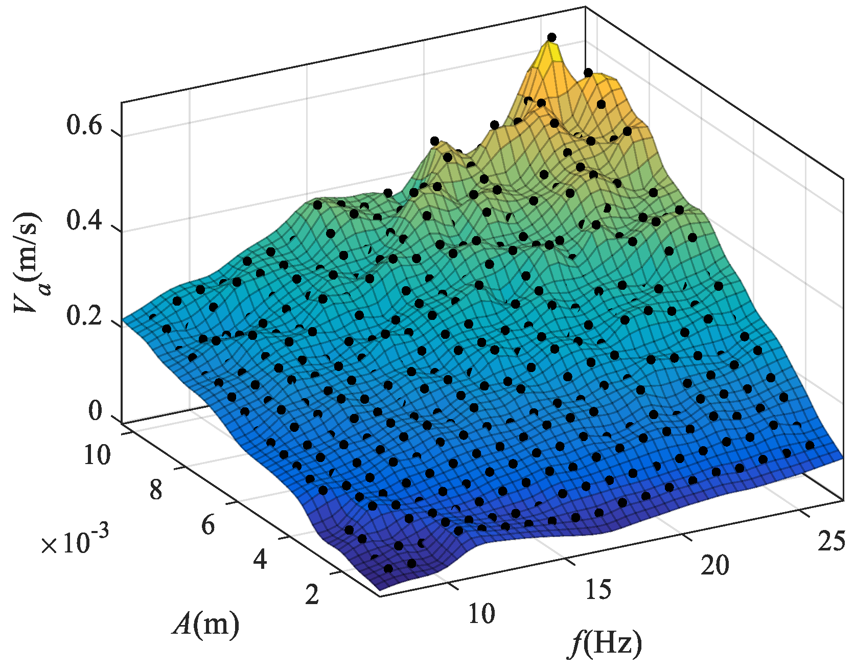
3.4. Effects of Frequency on the Dynamic Behavior of P–VS System

The dynamic behavior at 4 mm amplitude and 6–26 Hz frequency is discussed in this section. Figure 5a shows the bifurcation diagram of different frequencies at A = 4 mm, θ = 10°, a = 90°, and f_c = 0.5. According to Figure 5b,c, the particle motion exhibits quasiperiodic motion at a frequency of 6 Hz, and the particle bounces 5 times each period, in which one period is approximately 1/6 s. Moreover, the Poincaré map shows a circular dot area within y = 0.95 − 1.17 × 10⁻³ m. When the frequency increases to 6.5 Hz, the P–VS system changes from quasiperiodic motion to chaotic motion in which bifurcation occurs. As shown in Figure 5d,e, the particle bounces on the screening surface at any moment, and its Poincaré map resembles a semicircular ring above a small foot. When the frequency increases to 8 Hz, its nonlinear dynamic behavior is the same as the above content of the amplitude (Section 3.2), in which the Poincaré map shows a petal flower, as shown in Figure 5f,g. In addition, each mutation on the bifurcation diagram leads to one more petal on the Poincaré map. In short, the P–VS system presents quasiperiodic motion when working at low frequencies. When the frequency increases to 6.5 Hz, the bifurcation phenomenon occurs. At this time, the system presents chaotic motion, the attractor becomes larger, and the law is difficult to find. With a further increase in frequency, the attractor of the system becomes semicircular, and its Poincaré map becomes petal-shaped. After this stage, an increase in frequency will only increase the radius of the semicircle of the chaotic attractor and the number of petals on the Poincaré map.

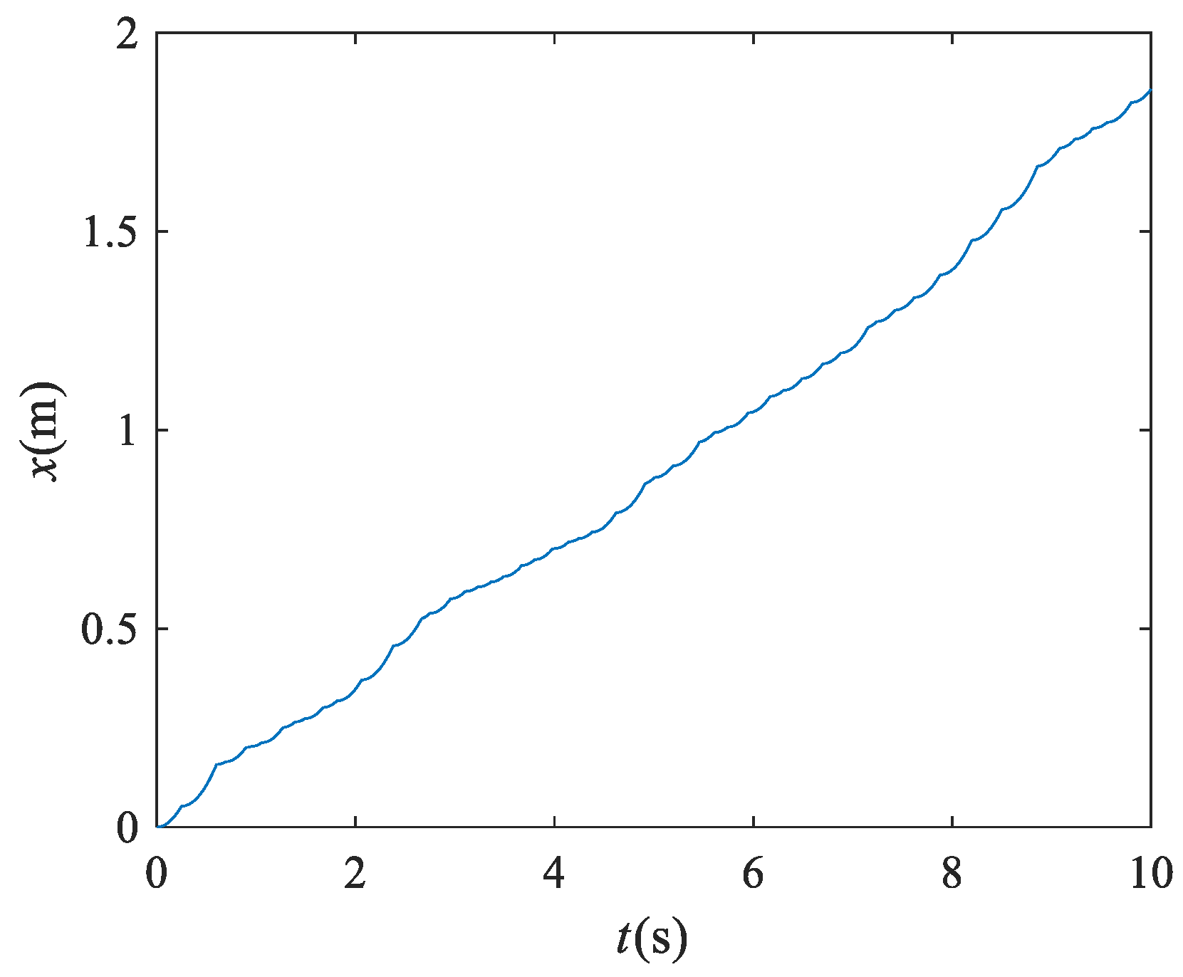
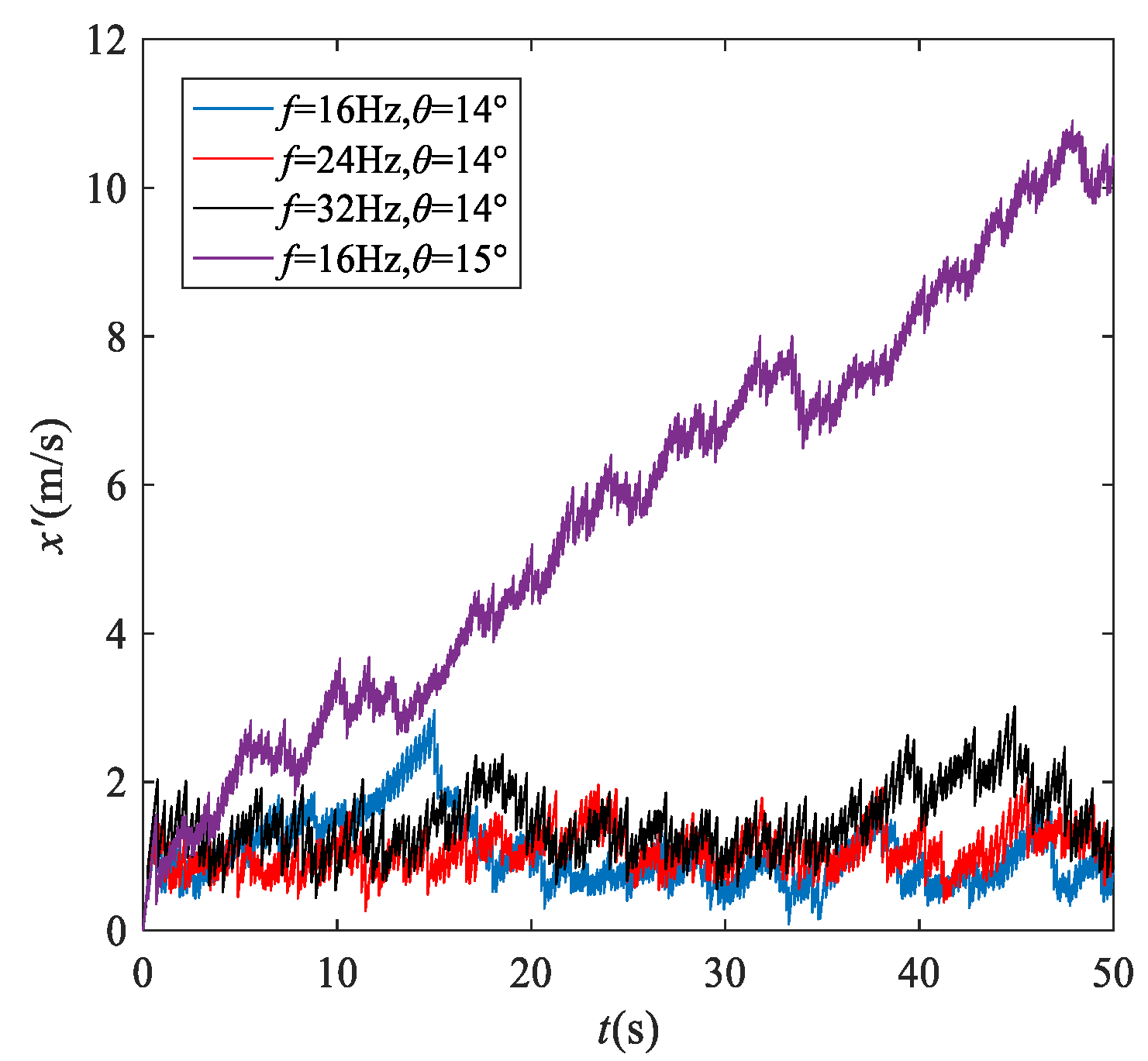
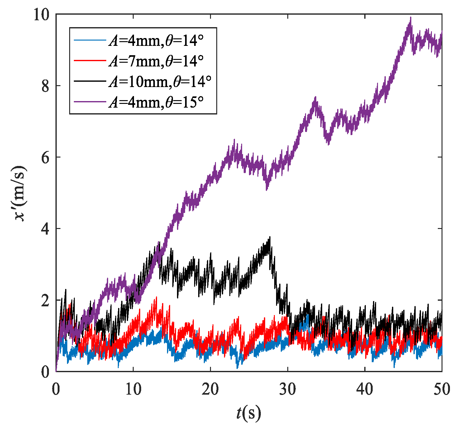
3.5. The Dynamic Behavior of a Particle along the Screening Surface

In this section, the particle speed under the influence of amplitude, frequency, inclination angle, and friction coefficient along the screening surface is mainly discussed. Figure 6 shows the displacement of the particle at f = 16 Hz and A = 4 mm. Basically, the displacement of the particle keeps increasing at a constant speed, in which the average speed V_a is approximately 0.19 m/s. In addition, each bounce reduces the speed in the tangential direction, as shown in Equations (6) and (7).

Figure 7 shows the average speed with A = 1–10 mm, f = 8–26 Hz, θ = 10°, and a = 90°. In general, the average speed of the particle increases with increasing amplitude and frequency. At low amplitude or low frequency, the rate of increase of the average particle speed is lower. Moreover, the amplitude has a greater effect on the particle speed compared to the frequency. However, there are distortion points in this process, and this phenomenon occurs more often at high frequencies and high amplitudes because the dynamic behavior of the particle is more difficult to predict under these conditions because of the strong nonlinearity of the dynamic system.

The figures and material presented above discuss the influence of common screening parameters (amplitude and frequency) on the average particle speed affected, furthermore, by an inclination angle, friction coefficient, and vibration direction angle. These parameters might not change in the actual screening process, but they have a large impact on the average particle speed. Figure 8 shows the influence of the inclination angle on the average particle speed in 5 s at A = 4 mm, f = 16 Hz, θ = 6–20°, and a = 90°. In general, the average particle speed increases with increasing inclination angle. At the same time, we found that a sudden increase occurs at θ = 14° because particle motion on the screening surface no longer converges, and 14° is the convergence threshold in this instance. Furthermore, we compare the convergence threshold of particle speed for different amplitudes and frequencies. Figure 9 shows the particle speed in 50 s at A = 5 mm, θ = 14°, 15°, a = 90°, and f = 16, 24, 32 Hz. The speed of the particle on the screening surface always converges with increasing frequency. The motion of the particle no longer converges when the inclination angle increases by 1°. These results show that the speed of convergence of particles is not strongly correlated with frequency, although an increase in frequency leads to an increase in speed. In contrast, the inclination angle has a great influence on the convergence threshold of the particle speed. Figure 10 shows the particle speed in 50 s at A = 4, 7, 10 mm, θ = 14, 15°, a = 90°, and f = 16 Hz. This figure illustrates that amplitude does affect the particle speed, but the amplitude and speed convergence threshold are slightly correlated. Similarly, we found that the vibration direction angle has little correlation with the convergence of the particle speed.

Furthermore, the friction coefficient affects the speed convergence threshold of the particle. Figure 11 shows the convergence condition of the inclination angle and friction coefficient at A = 5 mm, a = 90°, and f = 16 Hz. The particle speed converges when the value of the inclination angle and friction coefficient is below the curve, and the particle speed diverges to infinity when the value is above the curve. Meanwhile, the curve of the convergence condition is approximately linear, and the convergence threshold of the inclination angle increases with the friction coefficient.

Finally, the effect of the vibration direction angle on the average particle speed is discussed. Figure 12 shows the relation between the vibration direction angle and average particle speed at A = 4 mm, f = 16 Hz, θ = 10°, a = 90°, and f_c = 0.5. The average speed is minimal (V_a = 0.3637 m/s) when the vibration direction angle is 90°. When the vibration direction angle starts to tilt with the vertical direction of the screen surface, the average speed increases significantly and reaches the maximum speed (V_a = 0.7276 m/s) at a = 65°. The maximum average speed is almost twice the minimum average speed, which proves that the vibration direction angle has a large influence on the average speed. In the actual screening process, the granular material flow speed can be changed by adjusting the vibration direction angle. The average velocity begins to decrease and oscillates with a further reduction of the vibration direction angle.

4. Conclusions

In this research, the dynamic equations of a particle on a screening surface are established based on the elastoplastic contact model of round particles, and the dynamic behavior is discussed. We provide a theoretical method for studying the dynamic behavior of coal granular material on a vibrating screen. This method can be applied to other granular materials as well. The main conclusions are as follows:

(1)

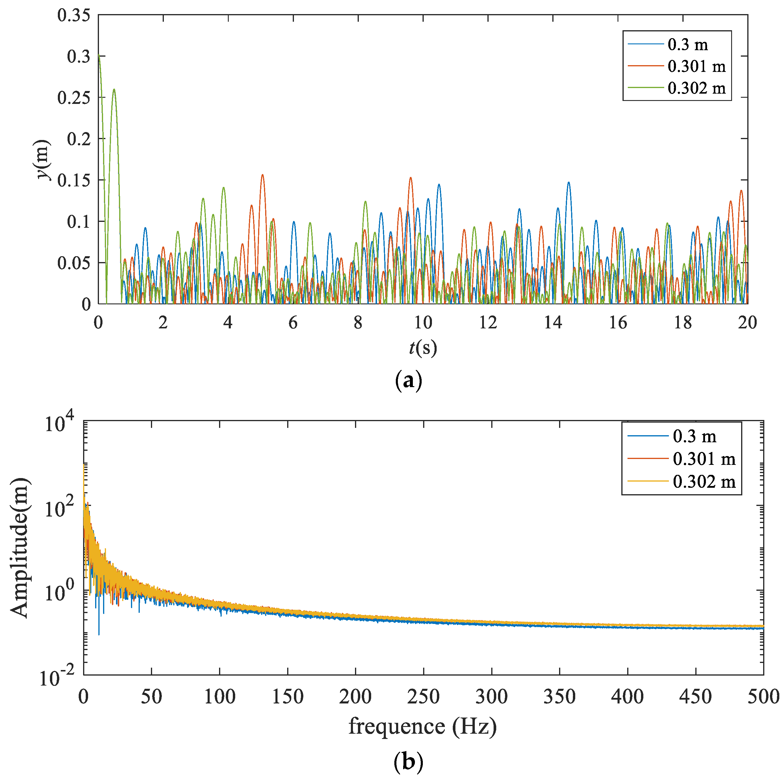
The P–VS system is strongly nonlinear. A small change in parameters, such as the initial falling height and radius of the particle, will significantly affect the trajectory of the particle.

(2)

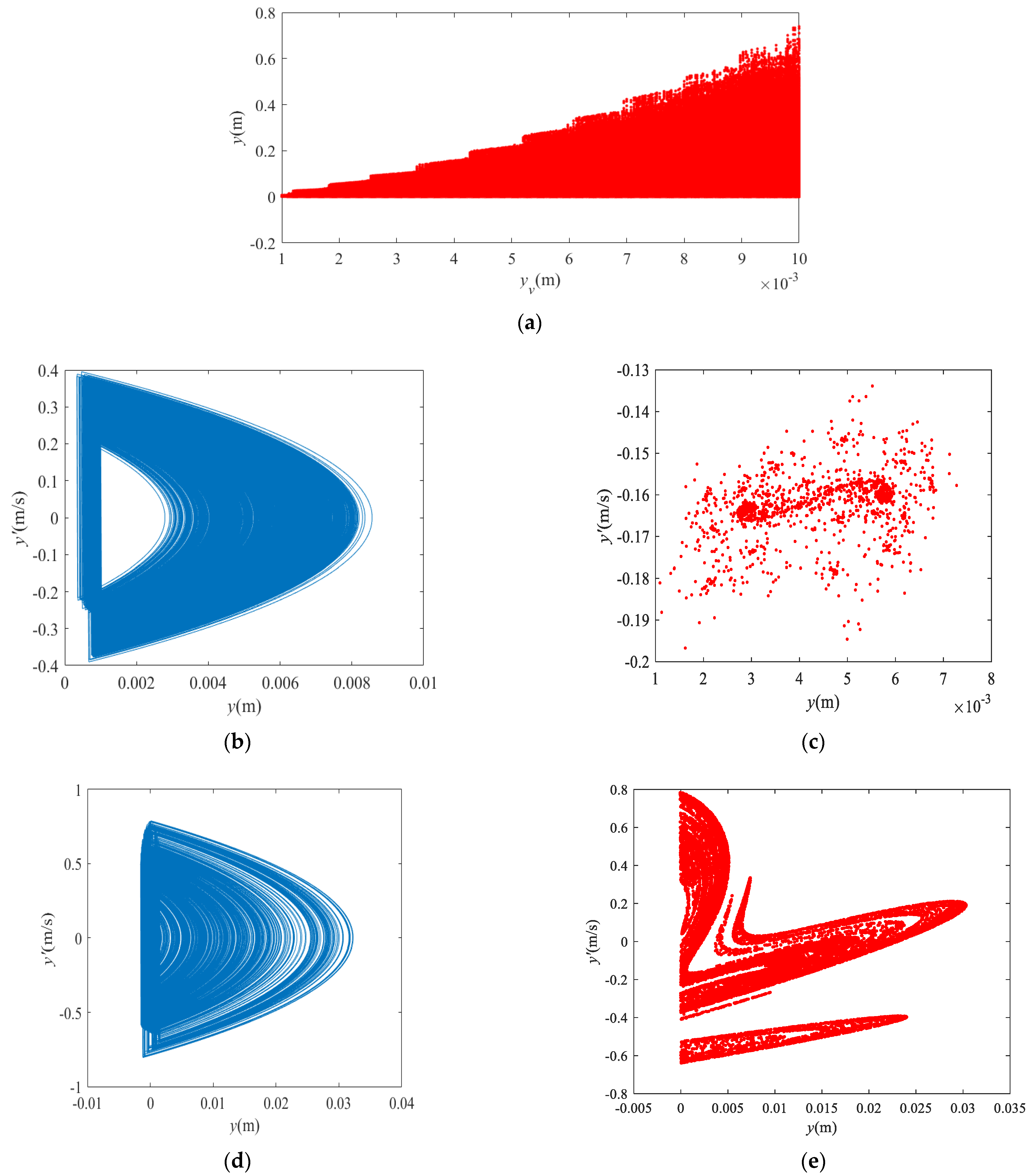
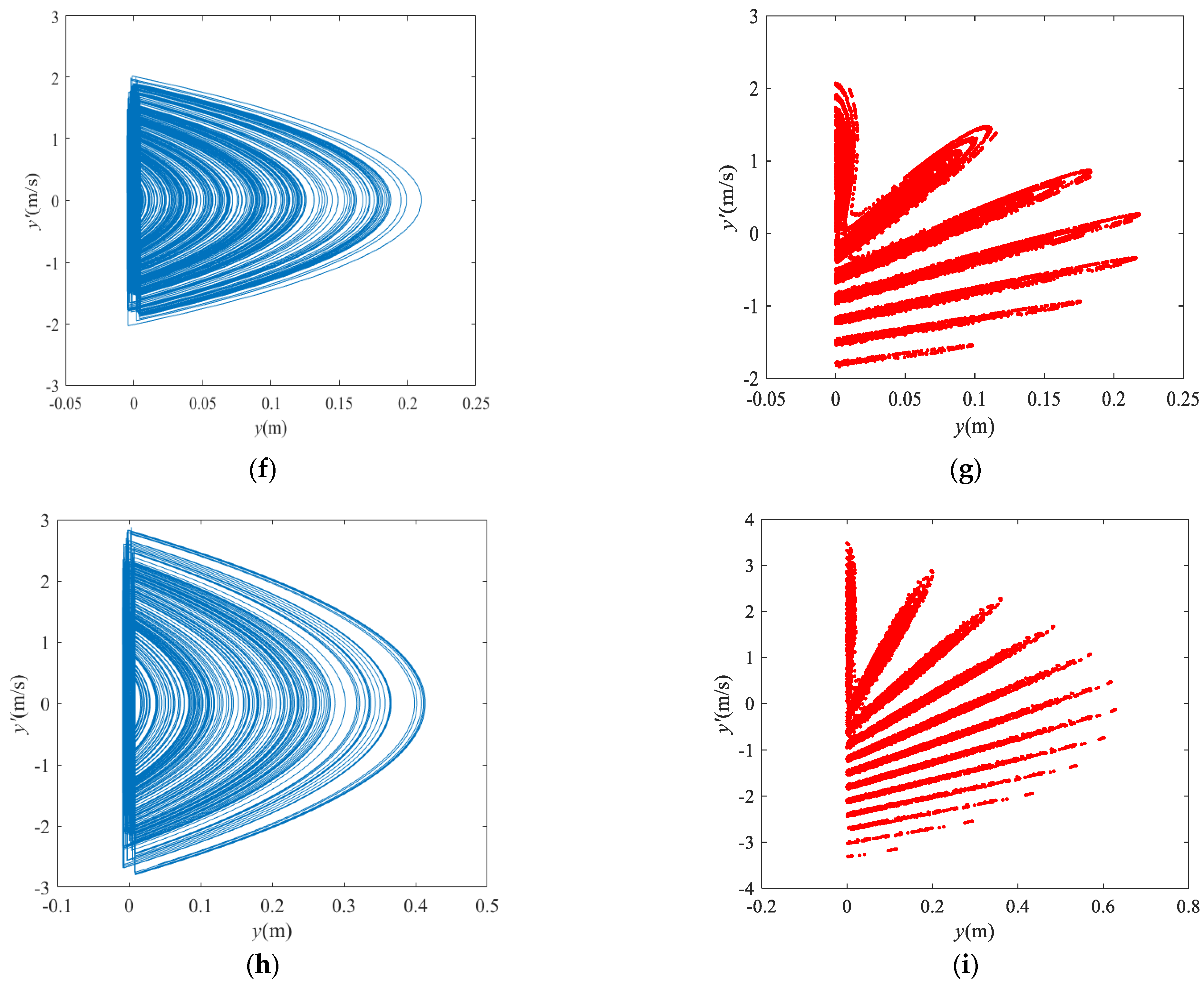
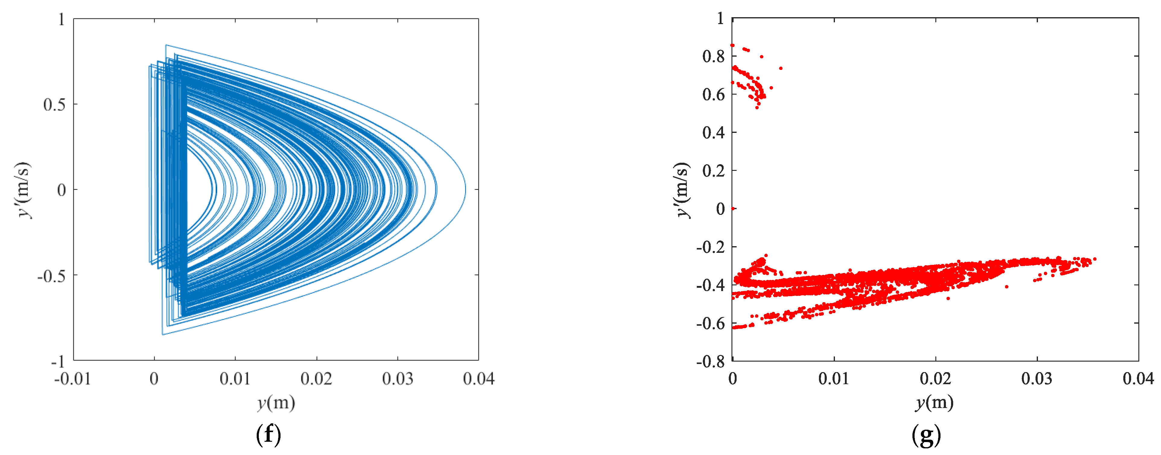
In the normal direction of the vibrating screen, the P–VS motion is quasiperiodic at low frequencies. With increasing frequency or amplitude, the motion of the P–VS system becomes chaotic, and its Poincaré map becomes petal-shaped. In addition, the number of petals increases at the mutation of the bifurcation diagram.

(3)

An increase in frequency, amplitude and inclination angle and a decrease in friction coefficient lead to an increase in particle speed along the screen surface. In addition, the particle speed reaches a maximum when the vibration direction angle is 65°.

(4)

The divergence and convergence of particle motion along the screening surface are only affected by the inclination angle and friction coefficient for the granular coal material.

In the future, the particle motion under optimal screening efficiency with different granular materials can be studied with our model. Whether the trajectories of different granular materials under optimal screening are similar merits verification.

References

1. Peng, L.; Wang, Z.; Ma, W.; Chen, X.; Zhao, Y.; Liu, C. Dynamic influence of screening coals on a vibrating screen. Fuel 2018, 216, 484–493. [Google Scholar] [CrossRef]
2. Chen, Z.; Li, Z.; Xia, H.; Tong, X. Performance optimization of the elliptically vibrating screen with a hybrid MACO-GBDT algorithm. Particuology 2021, 56, 193–206. [Google Scholar] [CrossRef]
3. Jiang, H.; Qiao, J.; Zhao, Y.; Duan, C.; Luo, Z.; Liu, C.; Yang, Y.; He, J.; Zhao, L.; Pan, M. Evolution process and regulation of particle kinematics and spatial distribution driven by exciting parameters during variable-amplitude screening. Powder Technol. 2018, 330, 292–303. [Google Scholar] [CrossRef]
4. Horenstein, M.N.; Mazumder, M.; Sumner, R.C. Predicting particle trajectories on an electrodynamic screen—Theory and experiment. J. Electrost. 2013, 71, 185–188. [Google Scholar] [CrossRef]
5. Jiang, Y.-Z.; He, K.-F.; Dong, Y.-L.; Yang, D.-l.; Sun, W. Influence of Load Weight on Dynamic Response of Vibrating Screen. Shock Vib. 2019, 2019, 4232730. [Google Scholar] [CrossRef]
6. Zhao, L.; Zhao, Y.; Bao, C.; Hou, Q.; Yu, A. Optimisation of a circularly vibrating screen based on DEM simulation and Taguchi orthogonal experimental design. Powder Technol. 2017, 310, 307–317. [Google Scholar] [CrossRef]
7. Pan, J.W.; Li, J.; Hong, G.Y.; Bai, J. A mapping discrete element method for nonlinear dynamics of vibrating plate-particle coupling system. Powder Technol. 2021, 385, 478–489. (In English) [Google Scholar] [CrossRef]
8. Jiang, H.; Yu, S.; Huang, L.; Zhao, Y.; Cao, X. Kinematics and mechanism of rigid-flex elastic screening for moist coal under disequilibrium excitation. Int. J. Coal Prep. Util. 2020, 42, 1724–1739. [Google Scholar] [CrossRef]
9. Wang, L.; Ding, Z.; Meng, S.; Zhao, H.; Song, H. Kinematics and dynamics of a particle on a non-simple harmonic vibrating screen. Particuology 2017, 32, 167–177. [Google Scholar] [CrossRef]
10. Yang, Y.; Wan, L.R. Study on the Vibroimpact Response of the Particle Elastic Impact on the Metal Plate. Shock Vib. 2019, 2019, 1–13. (In English) [Google Scholar] [CrossRef]
11. Dong, J.; Fang, J.; Pan, J.; Hong, G.; Li, J. Dynamic model of vibrating plate coupled with a granule bed. Chaos Solitons Fractals 2022, 156, 111857. [Google Scholar] [CrossRef]
12. GFF, G. Hertz’s Miscellaneous Papers. Nature 1896, 55, 6–9. [Google Scholar]
13. Hunt, K.; Crossley, E. Coefficient of restitution interpreted as damping in vibroimpact. J. Appl. Mech. 1975, 42, 440–445. [Google Scholar] [CrossRef]
14. Thornton, C. Coefficient of Restitution for Collinear Collisions of Elastic-Perfectly Plastic Spheres. J. Appl. Mech. 1997, 64, 383–386. [Google Scholar] [CrossRef]
15. Jian, B.; Hu, G.M.; Fang, Z.Q.; Zhou, H.J.; Xia, R. A normal contact force approach for viscoelastic spheres of the same material. Powder Technol. 2019, 350, 51–61. [Google Scholar] [CrossRef]
16. Safaeifar, H.; Farshidianfar, A. A new model of the contact force for the collision between two solid bodies. Multibody Syst. Dyn. 2020, 50, 233–257. [Google Scholar] [CrossRef]
17. Shen, Y.; Xiang, D.; Wang, X.; Jiang, L.; Wei, Y. A contact force model considering constant external forces for impact analysis in multibody dynamics. Multibody Syst. Dyn. 2018, 44, 397–419. [Google Scholar] [CrossRef]
18. Vu-Quoc, L.; Zhang, X.; Lesburg, L. Normal and tangential force–displacement relations for frictional elasto-plastic contact of spheres. Int. J. Solids Struct. 2001, 38, 6455–6489. [Google Scholar] [CrossRef]
19. Yang, Y.; Cheng, Y.M. A fractal model of contact force distribution and the unified coordination distribution for crushable granular materials under confined compression. Powder Technol. 2015, 279, 1–9. (In English) [Google Scholar] [CrossRef]
20. Ye, Y.; Zeng, Y.W.; Chen, X.; Sun, H.Q.; Ma, W.J.; Peng, Z.X. Development of a viscoelastoplastic contact model for the size- and velocity-dependent normal restitution coefficient of a rock sphere upon impact. Comput. Geotech. 2021, 132, 104014. (In English) [Google Scholar] [CrossRef]
21. Yu, J.; Chu, J.; Li, Y.; Guan, L. An improved compliant contact force model using a piecewise function for impact analysis in multibody dynamics. Proc. Inst. Mech. Eng. Part K J. Multi-Body Dyn. 2020, 234, 424–432. [Google Scholar] [CrossRef]
22. Zhang, J.; Li, W.; Zhao, L.; He, G. A continuous contact force model for impact analysis in multibody dynamics. Mech. Mach. Theory 2020, 153, 103946. [Google Scholar] [CrossRef]
23. Zhao, P.; Liu, J.; Li, Y.; Wu, C. A spring-damping contact force model considering normal friction for impact analysis. Nonlinear Dyn. 2021, 105, 1437–1457. [Google Scholar] [CrossRef]
24. da Silva, M.R.; Marques, F.; da Silva, M.T.; Flores, P. A compendium of contact force models inspired by Hunt and Crossley’s cornerstone work. Mech. Mach. Theory 2022, 167, 104501. (In English) [Google Scholar] [CrossRef]
25. Ji, S.; Liu, L. Contact Force Models for Granular Materials. In Computational Granular Mechanics and Its Engineering Applications; Ji, S., Liu, L., Eds.; Springer: Singapore, 2020; pp. 51–96. [Google Scholar]
Figure 1. Dynamic model of the particle-vibrating screening system.
Separations 09 00216 g001
Figure 2. Dynamic response of the particles with different falling heights: (a) the trajectories of the particles and (b) the frequency spectra of the particles.
Separations 09 00216 g002
Figure 3. Dynamic responses of particles with different radii.
Separations 09 00216 g003
Figure 4. Nonlinear behavior of a particle at different amplitudes: (a) Bifurcation diagram of different amplitudes; (b) Phase diagram at A = 1 mm; (c) Poincaré map at A = 1 mm; (d) Phase diagram at A = 1.5 mm; (e) Poincaré map at A = 1.5 mm; (f) Phase diagram at A = 5 mm; (g) Poincaré map at A = 5 mm; (h) Phase diagram at A = 9 mm; (i) Poincaré map at A = 9 mm.
Separations 09 00216 g004aSeparations 09 00216 g004b
Figure 5. Nonlinear behavior of a particle at different frequencies: (a) Bifurcation diagram of different frequencies; (b) Phase diagram at f = 6 Hz; (c) Poincaré map at f = 6 Hz; (d) Phase diagram at f = 6.5 Hz; (e) Poincaré map at f = 6.5 Hz; (f) Phase diagram at f = 8 Hz; (g) Poincaré map at f = 8 Hz.
Separations 09 00216 g005aSeparations 09 00216 g005b
Figure 6. Displacement of the particle at f = 16 Hz and A = 4 mm.
Separations 09 00216 g006
Figure 7. Average speed with A = 1–10 mm, f = 8–26 Hz, θ = 10°, and a = 90°.
Separations 09 00216 g007
Figure 8. Average particle speed in 5 s at A = 4 mm, f = 16 Hz, θ = 6–20°, and a = 90°.
Separations 09 00216 g008
Figure 9. Particle speed in 50 s at A = 5 mm, θ = 14, 15°, a = 90°, and f = 16, 24, 32 Hz.
Separations 09 00216 g009
Figure 10. Particle speed in 50 s at A = 4, 7, 10 mm, θ = 14, 15°, a = 90°, and f = 16 Hz.
Separations 09 00216 g010
Figure 11. Convergence curve of the inclination angle and friction coefficient at A = 5 mm, a = 90°, and f = 16 Hz.
Separations 09 00216 g011
Figure 12. Relation between the vibration direction angle and particle average speed at A = 4 mm, f = 16 Hz, θ = 10°, and fc = 0.5.
Separations 09 00216 g012