2.1. The Spaces
Let
D be a domain in
and
be the collection of all bivariate polynomials with real coefficients and total degree
,
Using a finite number of irreducible algebraic curves to carry out the partition Δ, we divide the domain
D into a finite number of sub-domains
. Each sub-domain is called a cell. The line segments that form the boundary of each cell are called the “edges”, and intersection points of the edges are called the “vertices”. The space of multivariate spline functions is defined by
A spline
s is a piecewise polynomial function of degree
k possessing continuous partial derivatives up to the order
in
D.
Suppose
for given positive integers
m and
n, endowed with the decomposition induced by the four-directional mesh
with grid lines:
We have the following result [
10,
23].
Theorem 1. For the bivariate spline space it holdswhere Since each interior grid point in
D is the intersection of exactly four lines from the grid partition
, the degree
k and the smoothness
must satisfy the relationship [
10]
It is easy to see that the spaces
have a locally supported basis [
10]. For
and
, we refer to [
10,
24,
25,
26,
27,
28] for more details. We discuss the spline spaces
in the following sections.
2.2. Basis of
By (
3), we get the dimension of
as follows:
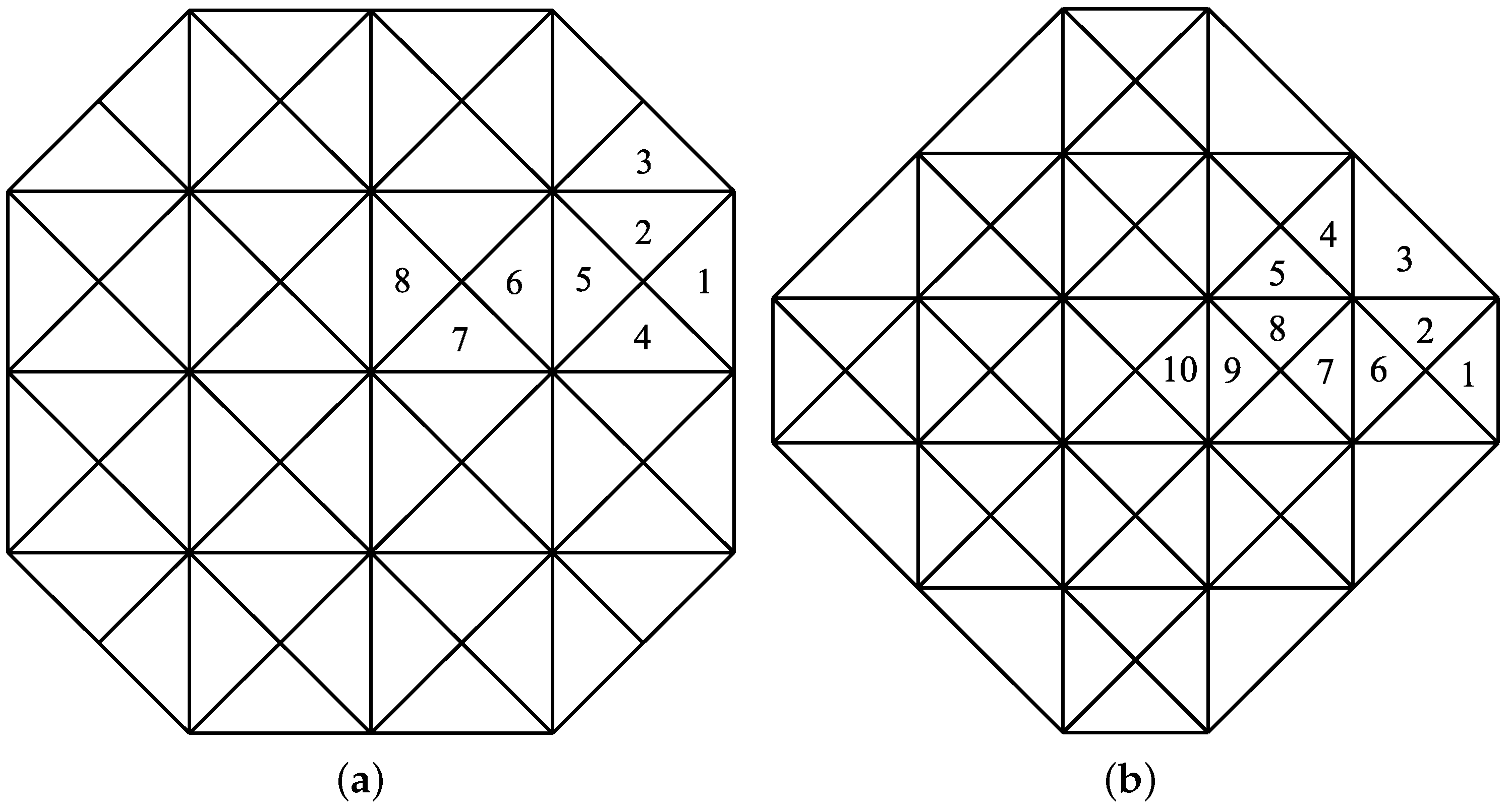
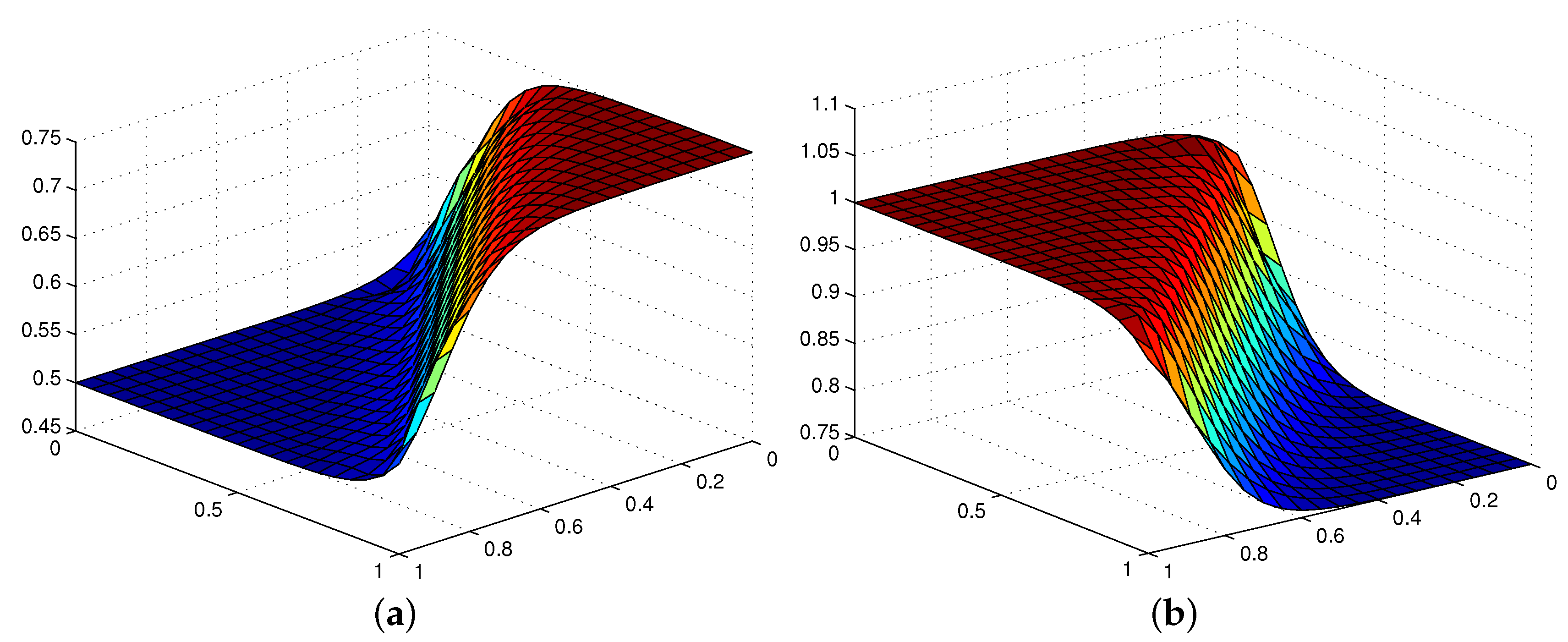
By using the smoothing cofactor–conformality method [
5,
10], we obtain two bivariate splines A and B whose supports are shown in
Figure 1a,b. The centers of the supports are
and
, respectively. Here, the considered domain
D is
. The local supports of
and
are minimal, and for
, there are four symmetry axes:
while, for
, there also exist four symmetry axes:
The restriction
of A to the cell
in
Figure 1a are as follows:
The restriction
of B to the cell
, in
Figure 1b are as follows:
The expressions of the restrictions of A and B to the other cells are obtained by symmetry.
Denote by
the translates of A and B, i.e., for all i,j
It is clear that the index sets for which the functions
and
do not vanish identically on
D are
Since the number of these splines is
, which is larger than the dimension of
, these splines are linearly dependent. For constructing a basis of
, we need to delete ten splines from the ones. We have the following result.
Theorem 2. LetThen, is a basis of . Since the cardinality of
is the same as the dimension of
, it is sufficient to prove that
is a linearly independent set on
D. This can be done by following the proof of Theorem 3.1 in [
29].
By checking the sums of the appropriate Bézier coefficients, we have the following identities:
2.3. Quasi-Interpolation Operators for
From the basis functions in the previous section, we can construct various kinds of quasi-interpolation operators.
Theorem 3. LetThen, for it holds In applications, a linear combination
of splines
and
is used [
30,
31]. It is given by
The support of
is the union of the involved splines
and
. The center of the support is
and the number of
does not vanish identically on
D is
, which is less than the dimension of
, so all
can only span a proper subspace of
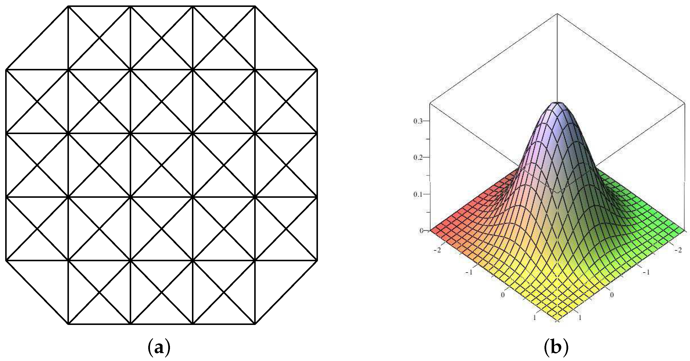
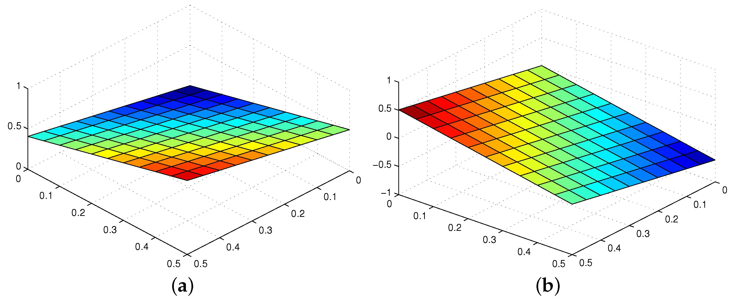
. The shape of one
is shown in
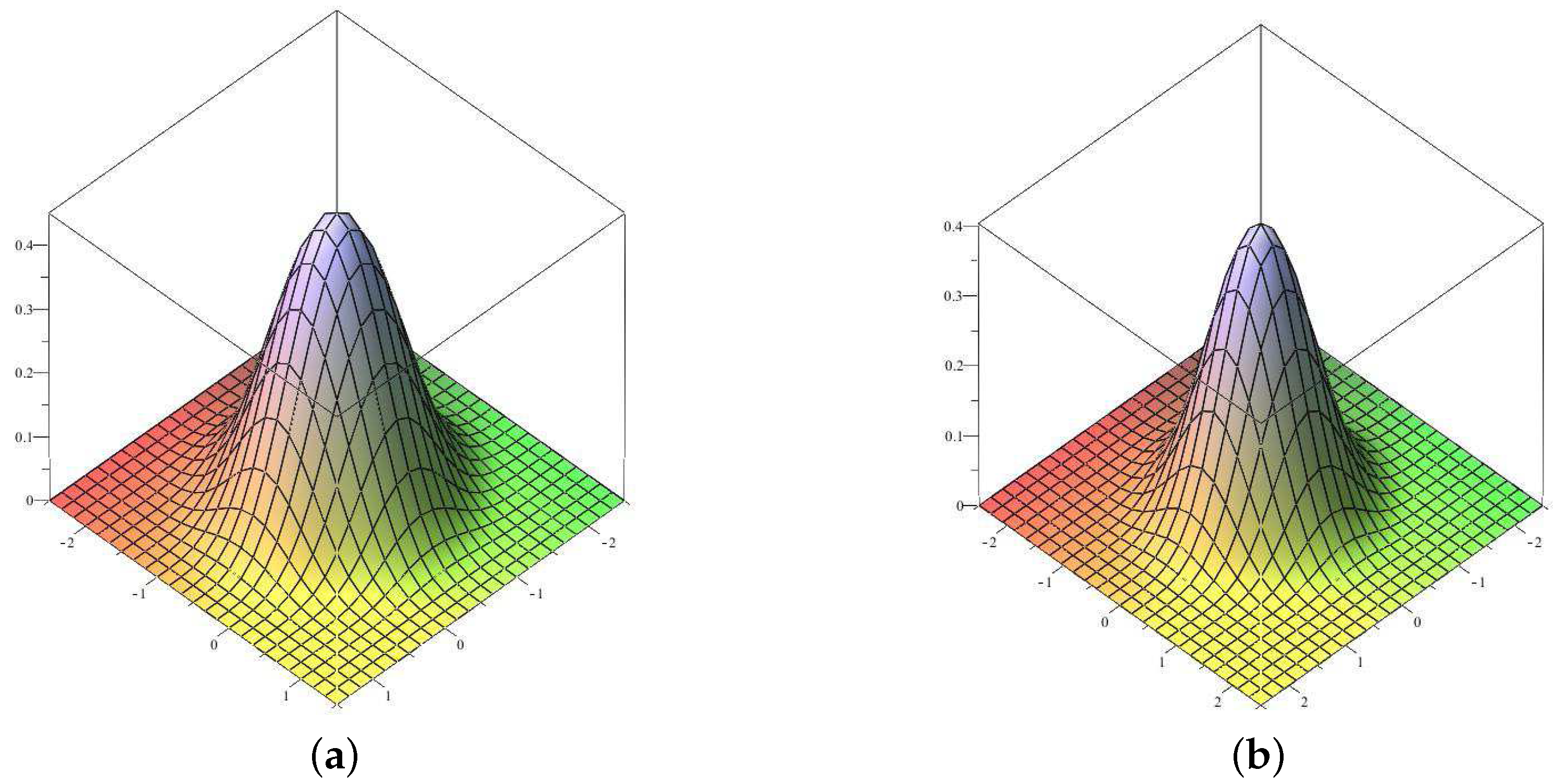
Figure 2b. The shapes of the splines
A and
B are displayed in
Figure 3. The splines
form a partition of unity.
It is worthwhile to note that, only using , we can construct higher precision quasi-interpolation operators by the following theorems.
Let Ω denote an open set containing
D and
. Define the variation diminishing operator
:
Note that
W is a linear operator, and by simple checking, we have the following results.
Theorem 4. For all , , we have In order to preserve identities for all polynomials in
and
, we define other kinds of linear operators
:
where
Note that each linear functional
depends on nine function values of
f at the grid points and the corresponding midpoints in the support of
. We have the following results:
Theorem 5. For all , ,we have There is a unique value of for which the corresponding operator is exact on .
Theorem 6. For all , ,we have Note that Theorem 6 has a better result than Theorem 5 but at the cost of using all nine function values. The conclusion of Theorem 5 can be used with flexibility, i.e., having the opportunity of choosing approximate
for given problems. The commonly used coefficients
of Theorem 5 are as follows:
We have the following result:
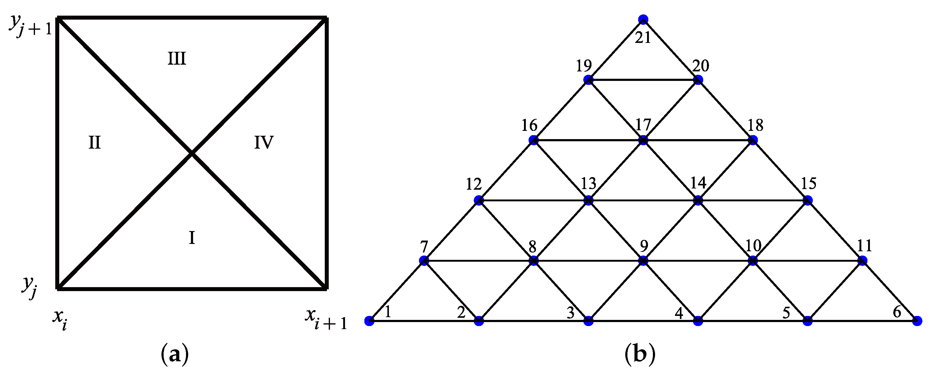
Theorem 7. For all , , we havewhere To prove Theorems 5–7, we need to testify the conclusions at each sub-region
(see
Figure 4a). For
I in
, we have a properly posed set of nodes for multivariate spline interpolation (21 points, see
Figure 4b) [
10]. Next, by computing the values of
in (
7) at these 21 points (noted by
), we get the fact that
. The same fact can be obtained similarly for
in
, respectively. Hence, these theorems hold by the arbitrariness of
.
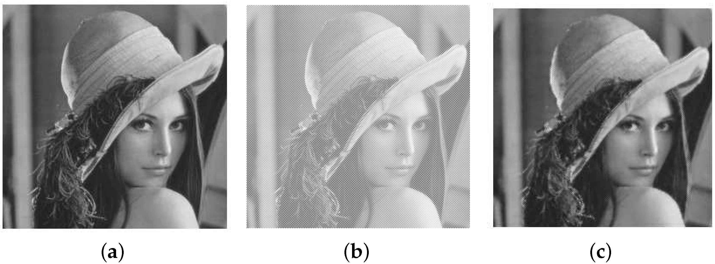
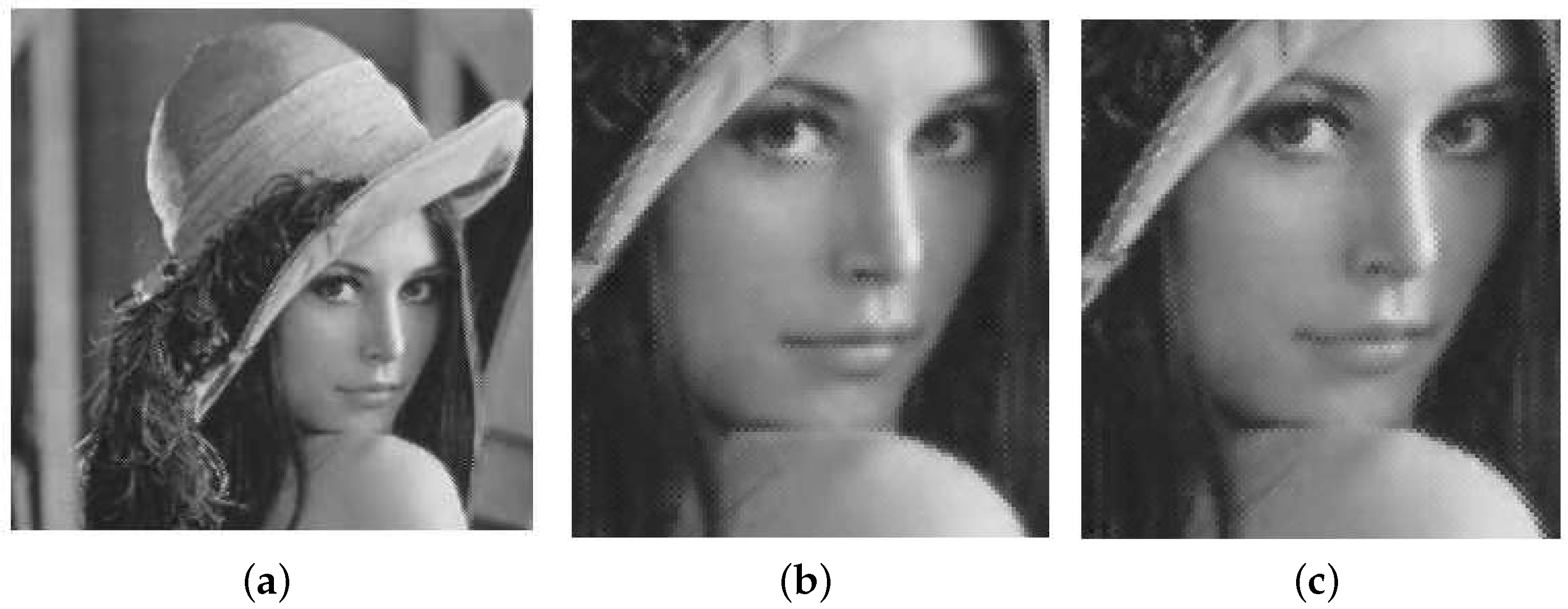
In the next section, we give two applications of the quasi-interpolation operator in Theorem 7.


