1. Introduction
The well-posedness of the continuous size-structured model has been studied in several papers (e.g., [
1,
2,
3,
4]). In Ref. [
1], authors proved the local existence and uniqueness of a solution of the continuous model, where birth and mortality functions depend on total population. In Ref. [
2], the authors established the local existence and uniqueness of a solution of the size-structured nonlinear population model, where also growth rate depends on total population. In the papers [
3,
4], the authors proved global existence and uniqueness of a solution of the continuous nonlinear population model, where all vital rates depend on total population. The total population can be described by e.g., total number of individuals (e.g., [
3]), total biomass (e.g., [
5]) or basal area.
A continuous nonlinear size-structured population model has been used in a forest management optimization problem (e.g., [
6,
7,
8]). In a continuous formulation, this nonlinear optimization problem cannot be solved by analytic methods. A natural approach is to solve this problem by approximating a continuous model by a discrete one and further solving a discrete optimization problem by iterative algorithms. In this paper, we focus on development of finite difference schemes to approximate the solution of a continuous nonlinear population model. Efficient schemes are essential for solving optimal control problems or parameter estimation problems as such problems require solving the model numerous times before an optimal solution is obtained.
When continuous population model is approximated by a finite difference scheme, it becomes a matrix population model [
9]. In matrix models, trees are divided into classes with respect to their size—for instance, diameter. The matrix describes how the class division changes at one time step. Matrix population models have also been used for forest management optimizations (e.g., [
10,
11]).
In optimization, using iterative algorithms is inevitable. Higher-order algorithms are usually sensitive to the regularity of the solution, and, therefore, they usually yield a convergence rate of first order as soon as the compatibility conditions are not satisfied. Moreover, in practice, the vital rates are determined on a statistical basis and the compatibility conditions required for high-order convergence are hardly valid with real-life data. These suggest that, in most cases, a first-order method should be the most adequate. Hence, it is desirable to have a robust scheme that can produce many useful qualitative and quantitative properties of the solutions of the differential problem but requires minimum regularity of the solution [
12]. Unfortunately, one could not derive the explicit formula for the optimal strategy since the strategy, the state and the costate are coupled into a complex system. The results at this stage may be regarded as a middle step to real world applications and serve as a starting point for numerical computations [
13].
In our knowledge, the comprehensive theoretical investigation of the forest management optimization problem with a continuous nonlinear population model as the state equation is still lacking, and, in that sense, the problem is an open problem. Hence, in this work, the investigation of the problem in its differential form is omitted, whereas, we consider the finite dimensional counterpart of the problem constructed by finite difference approximations of the state problem and taking for cost function a finite dimensional form used in practice. We prove the stability of constructed finite difference schemes on the set of non-negative solutions and solvability of the optimization problem, and deduce the necessary gradient information for iterative solution methods. We solve several applied problems, where different approximations schemes are used, and compare the computed results. The rest of the article is organized as follows. In
Section 2, a mathematical model of optimal harvesting problem for the size-structured forest is formulated. In
Section 3, we construct and investigate two finite difference approximation schemes for a nonlinear boundary value problem that simulates the growth and the harvesting of a forest. A gradient method for minimizing the cost function is constructed in
Section 4. The theoretical details of this method are set out in the
Appendix A to the article.
Section 5 is devoted to the numerical solution of a real-life problem and comparative analysis of the computing results. Finally, in
Section 6, we present discussions.
2. Formulation of the Optimal Control Problem
In order to formulate the mathematical model for the optimal harvesting problem for the size-structured forest, we define the following notations. In space, we denote by
the thickness of the tree, where
and
L are the lower and upper bounds of the space domain, respectively. Moreover,
is the time, where
T is the upper limit. By
Q, we denote the product space
. We denote by
and
the number of trees per unit area (state) and the number of removed trees per unit area (control), respectively. Now, the optimal harvesting problem where the cost functional
characterizes a net present value (NPV) of ongoing rotation, and
is the discounted price function, is formulated as follows:
Above
is the set of constraints for the state and the control, where
From the point of real-life problems, it is obvious that there exist constants
and
B, which denote the upper limit for harvesting and lower limit for making profitable thinning of trees at time event
t; otherwise, the thinning is not done. Notice that harvesting
h depends on the state
y (via constraint sets), which is defined by the population model
where
is growth rate,
mortality rate and
is initial diameter distribution of the trees. Growth and mortality rates depend on diameter
x of a tree and on the basal area,
, of the forest stand, where
In the case
, the problems (
4)–(6) are a particular case of the problem that have been investigated in [
1,
2,
3,
4]. In these articles, the existence of a non-negative continuous solution of this problem has been proved under some "natural" assumptions for input data. They are:
is continuous and strictly positive for all x and P and continuously differentiable with respect to x;
is non-negative for x and P and integrable in x;
and are Lipschitzian with respect to P;
.
We also assume that these assumptions are satisfied. We use growth rate
g and mortality
m in a bilinear form
where the constants
and
are such that
and
for all
and
. Obviously, because of suppositions
the boundary condition (5) reads as
.
The optimal harvesting problem has been investigated in [
6,
7,
8]. The authors of these publications considered the case where the harvesting function has the form
, where
is the control. Thus, they investigated a coefficient identification problem while we solve an optimal control problem with distributed (on the right-hand side) control.
3. Finite Difference Approximations
In this chapter, we derive explicit and (semi)implicit finite difference approximations for the state problems (
4)–(6) and prove their stability estimates on non-negative solutions. The investigation of existence, uniqueness and convergence of approximations is beyond the scope of our article. For the size-structured population model with recruitment, the existence, uniqueness and convergence of explicit approximations is investigated in [
14] and implicit approximation in [
5,
15].
The following notations are used throughout the paper: and denote the temporal and spatial mesh size, respectively. The non-overlapping mesh intervals are , , and , , where .
Let us denote by and the finite difference approximations of and , respectively. Moreover, we denote and the discrete values of the growth rate and mortality rate, respectively, in size class . The discretized value of the basal area at time is .
3.1. Explicit Approximation of the State Equation
For all meshpoints
the explicit finite difference approximation of the size-structured population model (
4)–(6) reads
Note that we use so-called upwind approximation for the first order derivative in space (variable
x) using the positivity of coefficient
on the set of non-negative mesh functions
y. The explicit scheme (
7) can be written in the form:
Later on, we denote by
. Moreover, we denote by
,
the vectors of the nodal values and by
the matrix of coefficients. Now, we can write explicit difference scheme (
7) in the following algebraic form:
Note that this scheme is just the forest growth model studied in [
11]. Moreover, the numerical calculation of the next temporal state involves only matrix to vector calculations. The drawback of the explicit scheme is that the following stability condition (
9) must be satisfied.
Lemma 1. Let the conditionbe satisfied. Then, on the set of non-negative mesh functions y, the finite difference scheme (7) is stablewhere . Proof. On the non-negative mesh functions
y, the coefficients
are positive and
. For the mesh steps satisfying condition (
9), the diagonal entries of matrix
satisfy the inequality
Because of this inequality, we have the following estimate for
-norm of matrices, connected with
-norm of vectors:
with
Due to this estimate and condition (
9), we obtain from Equation (
8) the inequality
whence stability estimate (
10) follows. ☐
The condition (
9) means that the length of the time step
and width of the size class
have to be chosen so that a tree cannot grow over one size class during one time step
(compare with [
16]).
3.2. Implicit Approximation of the State Equation
For all meshpoints
the implicit finite difference approximation of the models (
4)–(6) is the following linearized problem, with nonlinear coefficients calculated on the previous time level:
Equation (
11) can be rewritten as
Using the notations
we rewrite Equation (
11) in a form of linear algebraic equations
where
is a matrix of nonlinear coefficients.
Lemma 2. Finite difference scheme (11) is unconditionally stable on the set of non-negative mesh functions y: for any and the following stability estimate holds: Proof. By direct calculations, we obtain from Equation (
12) the equality
Since
and
, then, from this equality, we get
Because of positivity of vectors
and
the last inequality can be written in the form
whence stability estimate (
13) follows. ☐
Notice, contrary to the explicit scheme the time step
and class width
has no mutual dependence, hence the growth of a tree during a time step is not restricted less than one size class. This characteristic of the implicit scheme is useful in the optimal harvesting problem, covered by the models (
4)–(6) or parameter identification problem because such problems require solving the model many times before an optimal solution is obtained.
3.3. Approximation of the Optimal Control Problem
We denote
the discounted price for size class
at time
, and
. Moreover,
is the vector product of vectors
. Approximating the cost function (
1) by the right-hand Riemann sum, we get the following approximation for the harvesting problem:
Above, we denote by
, where
Moreover, and .
The following propositions show that the discrete optimal harvesting problem (
14) has at least one solution in both cases, i.e., if models (
4)–(6) is approximated explicitly or implicitly.
Proposition 1. Let the mesh steps and satisfy the inequality Then, Problem (
14)
has at least one solution if satisfies Equation (
7).
Proof. The set
K is non-empty. In fact, due to assumption (
17), the solution
of finite difference scheme (
7) with
is non-negative if
. This statement can be easily verified using form (
8) of the difference scheme and noting that all entries
and
of the matrices
are non-negative.
Obviously, assumption (
9) follows from inequality (
17), so stability estimate (
10) holds. Since vector
is bounded, then, due to inequality (
10), there exists a constant
Y such that
, i.e., the set
K is bounded. It is closed because of the continuity of functions
and
with respect to
while
P is obviously continuous with respect to
Thus,
K is compact. At last, cost function
of Problem (
14) is continuous, whence the existence of a solution to Problem (
14) follows from Weierstrass’s theorem. ☐
Proposition 2. Problem (
14)
has at least one solution if satisfies Equation (
11).
Proof. Proof is very similar to the proof of Proposition 1. Namely, the set
K is non-empty because, for
the solution
of finite difference scheme (
11) is non-negative for all
and
. Since
is bounded, then, due to stability estimate (
13),
is also bounded, so the set
K is bounded. It is closed because of the continuity of functions
and
with respect to
and continuity of
P with respect to
Thus,
K is compact. At last, cost function
of Problem (
14) is continuous, whence the existence of a solution to Problem (
14) follows.
Remark 1. Since neither the function is strictly concave nor the set K is strictly convex, the optimization problem can have a non-unique solution.
4. Realization of the Optimal Strategies
In this section, a first order method to approximate the optimal harvesting problem (
14) is constructed. In real-life applications, the growth rate
g and mortality rate
m are determined on a statistical basis and the compatibility conditions required for high-order methods can be hardly validated. Hence, a first order method, which is desirable to have a robust scheme but requires minimum regularity of the solution should be the most adequate. The first order methods require computing of the Fréchet derivatives (Jacobian matrix), which can be computationally expensive. However, when we consider the nonlinear optimization problem, only the gradient of the object function is needed, and the gradient can be computed without the Fréchet derivatives. In this work, the adjoint approach developed in the 1970s in [
17] is applied for calculation of the functional gradient. The adjoint method has a great advantage against the direct method because only one linear state problem, so called adjoint state, need to be solved for obtaining the gradient information. Today, it is a well-known method for computing the gradient of a functional with respect to model parameters when this functional depends on those model parameters trough state variables, which are solutions of the state problem. However, this method is less well understood in the control of population models, and, as far as we know, no applications to distributed optimal control of harvesting is presented in literature. Duality and adjoint equations are essential tools in studying existence of the optimal pair
, and, for a periodic age-dependent harvesting problem and for age-spatial structured harvesting problem, it is applied for proving the existence of the bang-bang control in [
18] and in [
19,
20], respectively. For continuous size-structured harvesting, problem duality and adjoint equations are applied for proving the existence of the bang-bang control in [
6,
8].
In this work, we apply the Lagrange method and give a recipe to systematically define the adjoint state equations and gradient information. We formulate the Lagrangian of the problem (
14) with respect to the state constraint (
15) only, and use the projection method regarding the control constraint (16). In the projection method, if solution goes outside the constraint set (16), it is projected back to there. Let us generalize and denote by
the operator Equation (
8) (or Equation (
12)). Moreover,
is the operator equation at the time level
.
Suppose the functional
and operator
A to be differentiable in the sense that there exist the following partial derivatives:
for all vectors
and
(or at least for the vectors such that
and
). Note that for the fixed
and
,
and
are vectors while
and
are matrices. By
and
, we denote the corresponding transpose matrices.
Let us define Lagrange function,
, of the problem (
14) by
where
. Now, for all feasible pair
holds
, and, for any
, we have:
and, since
does not depend on
, we have
Above, one method to approximate is to compute N finite differences over control variable . However, each computation requires solving the equation , and, for large N, this method is computationally expensive. In the adjoint method, we can avoid to compute by solving the linear adjoint state equation only once.
The theory of constrained optimization, see [
21], says that
is the optimal pair for the problem (
14) if
is a saddle point of
. The derivatives of
with respect to
,
and
are:
Now, gives the state equation, gives the adjoint state equation and gives the gradient.
Now, the calculation of the gradient can be summarized by the following steps when the Lagrangian is first formulated:
- I
Solve the state equation ;
- II
Solve the adjoint state equation
- III
Partial derivatives of
and
are presented in
Appendix A. Gradient
we used in projected gradient method [
22], which we applied for iteration of a solution of the optimal harvesting problem.
5. Numerical Example
In this section, we study numerical examples of problem (
14). We compared two cases where the state constraint (
4) was approximated with explicit approximation (
7) and implicit approximation (
11). As the discounted price for size class
at time
, we used
, where
r is the interest rate,
and
are the prices of the pulpwood and sawlog, respectively, and
and
are the volumes of pulpwood and sawlog of a tree in size class
, respectively. In the optimizations, we used the following values for parameters: price of pulpwood
€m
and sawlog
€m
, interest rate
and lower bound for harvested trees
m
ha
. The pulpwood and sawlog volumes
and
we got from [
10]. The optimization results of problem (
14) are presented in
Table 1 and
Table 2, and in
Figure 1 and
Figure 2.
The results show that the maximum net present value (NPV) associated with the explicit approximation (
7) was higher than the corresponding of the implicit approximation (
Table 1). When class width or time step decreased, maximum NPV increased in both cases. The difference of maximum NPVs between the two cases decreased when class width or time step decreased. Only when time step decreased from three to two years, the difference of maximum NPVs increased. The difference was biggest (99 €) when time step
years and class width
cm and smallest (28 €) when time step
years and class width
cm.
With both approximations, three or four intermediate thinnings were made (
Table 2). Number of thinnings increased when time step and class width decreased. When implicit approximation (
11) was used, first thinnings were made 1–2 time steps earlier, while the last few thinnings were made 0–2 time steps later than when explicit approximation (
7) was used. The thinning intensities were almost identical between the two approximations. If there was some difference, intensity was usually bigger when explicit approximation (
7) was used (
Table 2). The thinning pattern was in all optimal managements quite similar: in each thinning, more big trees than small ones were removed indicating a thinning from-above method (for different thinning types, see e.g., [
23], pp. 727, 733). Thinning from above has proven to be the best thinning type in stand-level optimizations of even-aged boreal forests (e.g., [
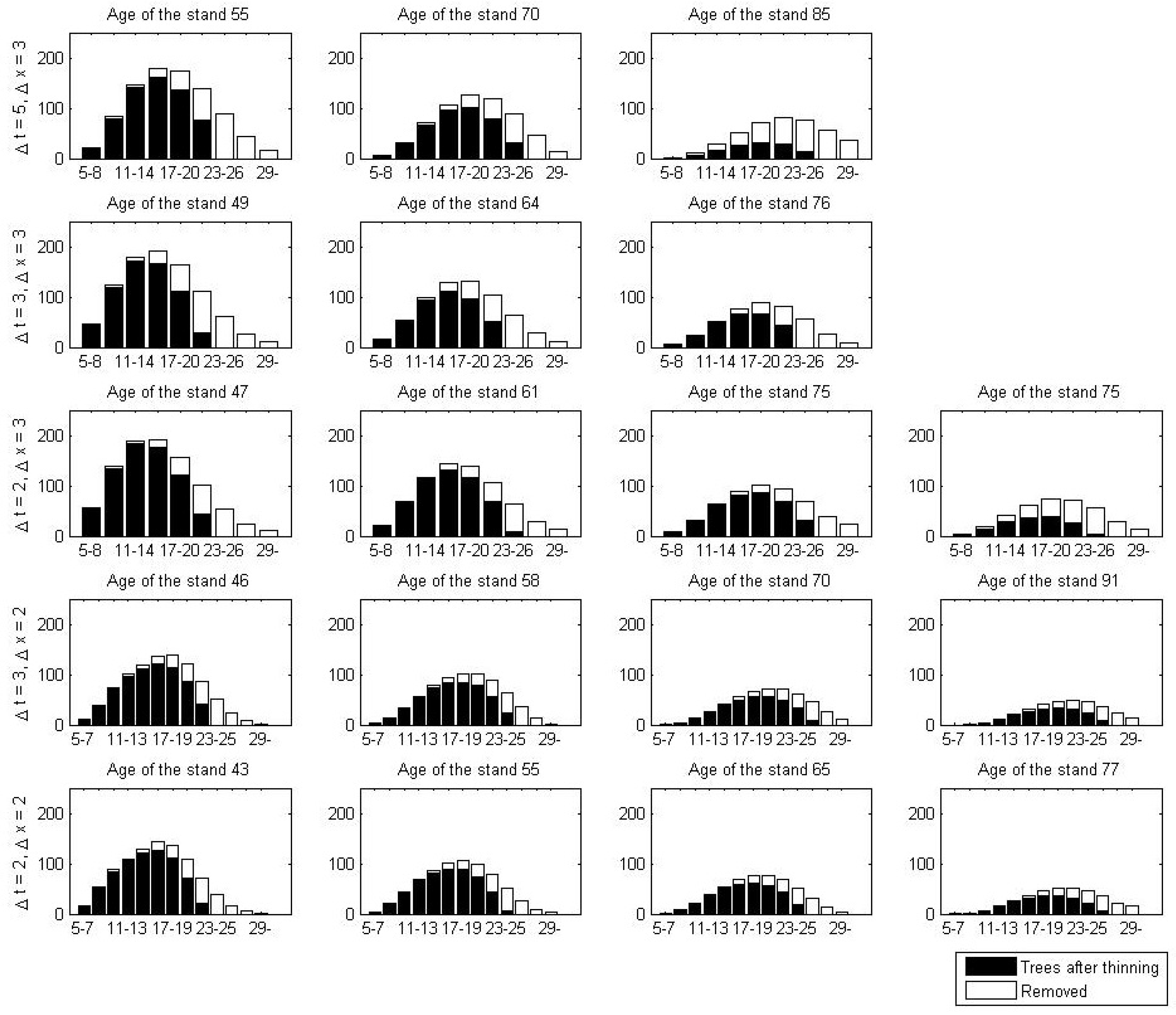
24]). When explicit approximation (
7) was used, all trees from two or three of the biggest size classes were removed (
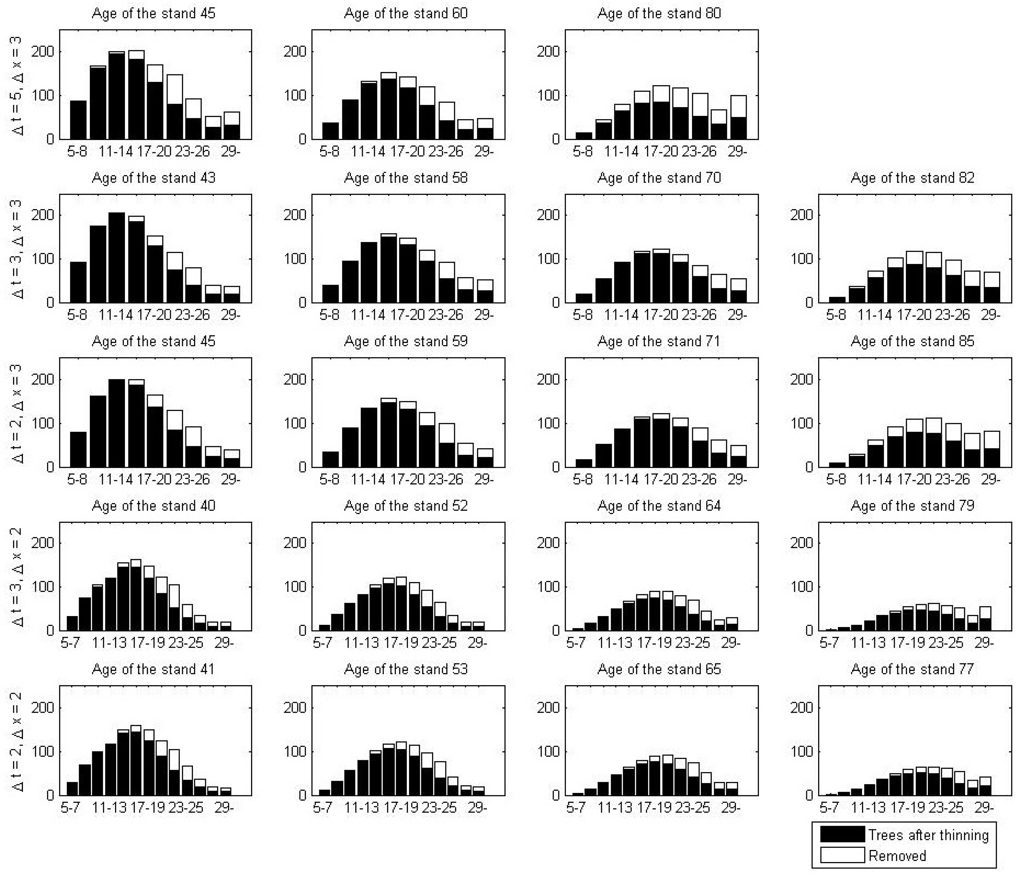
Figure 1). On the other hand, when implicit approximation (
11) was applied, only part of the trees from those size classes were removed (
Figure 2).
6. Discussion
This study contributes to existing literature on forest management by providing a theoretically sound framework to solve nonlinear optimization problem of even-aged stands. We compared the results of forest management optimizations, when the explicit and implicit approximations of the forest growth model was used. The optimization results show that the differences of the results between approximations are diminutive. This was expected as solutions of both approximation equations are proved to converge to solutions of continuous equation [
5,
14].
In numerical examples, we used data from the Scots pine (
Pinus sylvestris L.) stands that were located in Northern Ostrobothnia, Finland, on nutrient-poor soil type. The data was the same as in [
11]. The difference is that, in [
11], data was fitted directly to the matrix model, as, in this study, we first fitted data to the continuous model and then approximated it with a matrix model. In [
11], the time step was five years and class width 3 cm. The results are in line with each other. Both methods gave four thinnings in optimal management and thinning from above dominated as the thinning type. In [
11], the optimal net present value was slightly higher and, in the optimal management, the thinnings were made slightly earlier than in this study.
The optimal harvesting problem with a continuous size-structured population model was studied in [
6,
7,
8]. In those papers, harvesting was defined as a proportion of removed trees. The maximum principle for the problem was proved in [
6,
8]. Moreover, in [
7], the strong bang-bang principle under some additional (but realistic) conditions was proved. This means that the optimal solution has the structure, where all trees bigger than some certain size are removed. In our results, the solution of the optimization problem, where state constraint was approximated with explicit approximation, was nearer that structure. In addition, the optimization results were a little better then. However, when explicit approximation is used, the time step and class width have to be chosen so that a tree cannot grow over one size class during one time step [
16]. We proved that only then is the explicit approximation scheme stable. For the implicit approximation scheme, we proved that it is unconditionally stable. Thus, in implicit approximation, the time step and class width can be chosen freely. In general, explicit approximation of the population model is more commonly used as a forest growth model [
9,
16].


