Metrics for Single-Edged Graphs over a Fixed Set of Vertices

Abstract

Graphs have powerful representations of all kinds of theoretical or experimental mathematical objects. A technique to measure the distance between graphs has become an important issue. In this article, we show how to define distance functions measuring the distance between graphs with directed edges over a fixed set of named and unnamed vertices, respectively. Furthermore, we show how to implement these distance functions via computational matrix operations.

1. Introduction

When investigating the measurement of the distances between two sentences or structures, we feel it is necessary to first form a system to measure the distance for tree or graph structures. This was our initial motivation for developing this paper. This will provide a sound foundation and measurement technique for future applications. For example, if there are two separate English sentences, such as $S_1$ and $S_2$, and we would like to measure the distance between these two sentences, we identify $S_1$ with one graph and $S_2$ with another graph. Their vocabularies in individual sentences can be associated with vertices in the graph. The distance between the vocabularies can be identified with edges of the graphs. Then, we would have constructed graphs for $S_1$ and $S_2$. We would then be able to measure the distance between the two graphs. The main purpose of this article is to put forward an approach to define a metric for graphs on a fixed set of vertices.

Suppose V is a set of fixed vertices and E is a set of directed edges. Then, for each edge $(v,w)$, i.e., an edge from v to w, one can assign a value. Since most of the mathematical models can be formalized or represented via vertices and edges, studying the properties of the distances between any two graphs becomes a vital approach to explore the intrinsic properties of a mathematical structure or a real mathematical object [1,2], even being used on some fuzzy objects [3,4]. Some ingenious metrics for handling these fuzzy objects have been explored in depth [5,6]. In this article, we put forward two metrics for graphs with labelled vertices and unlabelled vertices, respectively. Nonetheless, we only consider the directed edges in this article. As for the indirected edges, one can simply treat them as pairs of two directed edges.

2. Definitions and Claims

We use ${\mathbb{R}}^{+}$ to denote all the positive real numbers. For any real number $\alpha$, we use $|\alpha |$ to denote its absolute value. For any set K, we use $\mathcal{P}(K)$ and $|K|$ to denote the power set and the size of K, respectively. If both H and K are sets, we use $H\to K$ to denote the set of all the functions from H to K. We use $H△K$ to denote $(H-K)\cup (K-H)$ (or $H-K\cup K-H$). We call $G=(V,E,W:E\to {\mathbb{R}}^{+})$ or in brevity $G=(V,E,W)$ a generalized graph, in which W is a weight function satisfying following conditions:

• For each $v\in V[(v,v)\in E\mathrm{and}W(v,v)=0]$;
• For all $(v_1,v_2)\in E[v_1\ne v_2\to W(v_1,v_2)>0]$.

Definition 1.

Let $GG(V)$ denote the set of all the generalized graphs whose vertex sets are exactly V.

Let $G_1=(V,E_1,W_1:E_1\to {\mathbb{R}}^{+}),G_2=(V,E_2,W_2:E_2\to {\mathbb{R}}^{+}),G_3=(V,E_3,W_3:E_3\to {\mathbb{R}}^{+})\in GG(V)$ be arbitrary generalized graphs. For any $G=(V,E,W:E\to {\mathbb{R}}^{+})\in GG(V)$ and any $a\in V$, we use $E(a)$ to denote the set of all the endpoints beginning from a, i.e.,

$$E(a)=\{b\in V:(a,b)\in E\}.$$

Furthermore, define the set of all the assigned values of $E(a)$ as follows:

$$W(a)=\{W(a,b):b\in E(a)\}.$$

3. Metric for Labelled Graphs

In this section, we assume all the vertices in V are labelled. We show how to define a distance between $G_1$ and $G_2$ as follows:

Definition 2.

(distance function: labelled vertices, single directed edge) Define $d_1:GG(V)\times GG(V)\to {\mathbb{R}}^{+}$ by

$$\begin{array}{c}{\displaystyle d_1(G_1,G_2):=\sum _{a\in V}[\sum _{c\in E_1(a)-E_2(a)}{W}_1(a,c)+\sum _{c\in E_2(a)-E_1(a)}{W}_2(a,c)+}\hfill \\ \sum _{c\in E_1(a)\cap E_2(a)}|W_1(a,c)-W_2(a,c)|].\hfill \end{array}$$

(1)

Example 1.

Suppose $V=\{v_1,v_2,v_3\}$ is a fixed set of vertices and graph $G_1=(V,E_1,W_1)$, and $G_2=(V,E_2,W_2)$, where their vertices assigned to the edges $E_1$, $E_2$ and the values for weights $W_1,W_2$ are given as follows:

$$\begin{array}{c}{E}_1=\{(v_1,v_2),(v_1,v_3),(v_3,v_1),(v_3,v_2)\},\hfill \\ E_2=\{(v_1,v_2),(v_2,v_1),(v_2,v_3),(v_3,v_2),(v_3,v_1)\},\hfill \\ W_1(v_1,v_2)=4,W_1(v_1,v_3)=3,W_1(v_3,v_1)=1,W_1(v_3,v_2)=7,\hfill \\ W_2(v_1,v_2)=3,W_2(v_2,v_1)=5,W_2(v_2,v_3)=3,W_2(v_3,v_2)=4,W_2(v_3,v_1)=6.\hfill \end{array}$$

Then, the end vertices originating from $v_1$ via edges in $E_1$ could be depicted as $E_1(v_1)=\{v_2,v_3\}$. Others follow:

$$\begin{array}{c}{E}_2(v_1)=\left\{v_2\right\},E_1(v_2)=\varnothing ,E_2(v_2)=\{v_1,v_3\},\hfill \\ E_1(v_3)=\{v_1,v_2\},E_2(v_3)=\{v_1,v_2\}.\hfill \end{array}$$

Henceforth, by Definition 1, one could compute the distance for $G_1$ and $G_2$ as follows: $d_1(G_1,G_2)=$

$$\begin{array}{c}\sum _{c\in E_1(v_1)-E_2(v_1)}{W}_1(v_1,c)+\sum _{c\in E_2(v_1)-E_1(v_1)}{W}_2(v_1,c)+\sum _{c\in E_1(v_1)\cap E_2(v_1)}|W_1(v_1,c)-W_2(v_1,c)|+\hfill \\ \sum _{c\in E_1(v_2)-E_2(v_2)}{W}_1(v_2,c)+\sum _{c\in E_2(v_2)-E_1(v_2)}{W}_2(v_2,c)+\sum _{c\in E_1(v_2)\cap E_2(v_2)}|W_1(v_2,c)-W_2(v_2,c)|+\hfill \\ \sum _{c\in E_1(v_3)-E_2(v_3)}{W}_1(v_3,c)+\sum _{c\in E_2(v_3)-E_1(v_3)}{W}_2(v_3,c)+\sum _{c\in E_1(v_3)\cap E_2(v_3)}|W_1(v_3,c)-W_2(v_3,c)|\hfill \\ =[W_1(v_1,v_3)+0+|W_1(v_1,v_2)-W_2(v_1,v_2)|]+[0+W_2(v_2,v_1)+W_2(v_2,v_3)+0]\hfill \\ +[0+0+|W_1(v_3,v_1)-W_2(v_3,v_1)|+|W_1(v_3,v_2)-W_2(v_3,v_2)|]\hfill \\ =[3+0+1]+[0+5+3+0]+[0+0+5+3]=20.\hfill \end{array}$$

Hence we have the result that the distance for $G_1$ and $G_2$ is 20 by metric $d_1$.

Claim 1.

For all $a\in V$, one has

$$\begin{array}{c}[(E_1(a)▵E_2(a))\cup (E_1(a)\cap E_2(a))]\cup \hfill \\ [(E_2(a)▵E_3(a))\cup (E_2(a)\cap E_3(a))]\supseteq \hfill \\ [(E_1(a)▵E_3(a))\cup (E_1(a)\cap E_3(a))].\hfill \end{array}$$

Proof. 

It follows immediately from the fact that

$$(E_1(a)\cup E_2(a))\cup (E_2(a)\cup E_3(a))\supseteq (E_1(a)\cup E_3(a)).$$

 □

Claim 2.

(semi-metric)

1. 

$d_1(G_1,G_2)\ge 0$;

2. 

$d_1(G_1,G_2)=d_1(G_2,G_1)$;

3. 

$d_1(G_1,G_2)=0$iff$G_1=G_2$.

Proof. 

By the definition, the first and second statements follow immediately. Here we show the third statement. Suppose $G_1=G_2$. Then,

$${\displaystyle d_1(G_1,G_2)=\sum _{a\in V}[\sum _{c\in E_1(a)\cap E_2(a)}|W_1(a,c)-W_2(a,c)|]=0.}$$

On the other hand, if $d_1(G_1,G_2)=0$, then $\forall a\in V[E_1(a)=E_2(a)]$ and $W_1=W_2$, i.e., $G_1=G_2$.  □

From above inferences, if one allows $W(v,w)=0$ for some $v\ne w$, then $d_1(G_1,G_2)=0\Rightarrow G_1=G_2$ might not hold in some particular $G_1$ and $G_2$. Similarly, if one allows $W(v,v)=0$, then for all $v\in V[(v,v)\in E]$ is a requirement.

Theorem 1.

$(GG(V),=,d_1)$ is a metric space.

Proof. 

Since we have shown in Claim (2) that $d_1$ is a semi-metric, it suffices to show $d_1$ satisfies the triangle property:

$$d_1(G_1,G_2)+d_1(G_2,G_3)\ge d_1(G_1,G_3).$$

(2)

On the basis of Claim (1), we have the following inferences. Let $a\in V$ be arbitrary. Firstly, if $c\in E_1(a)-E_3(a)$, then $c\in E_1(a)-E_2(a)$ or $c\in E_1(a)\cap E_2(a)$. If $c\in E_1(a)-E_2(a)$, then it preserves the inequality of Equation (2). If $c\in E_1(a)\cap E_2(a)$, then $c\in E_2(a)-E_3(a)$, i.e.,

$$c\in E_1(a)\cap E_2(a)\mathrm{and}c\in E_2(a)-E_3(a).$$

It follows that

$$|W_1(a,c)-W_2(a,c)|+W_2(a,c)\ge W_1(a,c),$$

i.e., the inequality of Equation (2) is preserved. Secondly, if $c\in E_3(a)-E_1(a)$, by the same analogy, the inequality of Equation (2) is also preserved. Lastly, if $c\in E_1(a)\cap E_3(a)$, then [$c\in E_1(a)-E_2(a)$ or $c\in E_1(a)\cap E_2(a)$] and [$c\in E_3(a)-E_2(a)$ or $c\in E_2(a)\cap E_3(a)$], i.e.,

$$c\in E_1(a)-E_2(a)\mathrm{and}c\in E_3(a)-E_2(a)$$

or

$$c\in E_1(a)\cap E_2(a)\mathrm{and}c\in E_2(a)\cap E_3(a).$$

It follows that

$$W_1(a,c)+W_3(a,c)\ge |W_1(a,c)-W_3(a,c)|,$$

$$|W_1(a,c)-W_2(a,c)|+|W_2(a,c)-W_3(a,c)|\ge |W_1(a,c)-W_3(a,c)|.$$

Hence, we have shown

$$\sum _{c\in E_1(a)-E_2(a)}{W}_1(a,c)+\sum _{c\in E_2(a)-E_1(a)}{W}_2(a,c)+\sum _{c\in E_1(a)\cap E_2(a)}|W_1(a,c)-W_2(a,c)|$$

$$+\sum _{c\in E_2(a)-E_3(a)}{W}_2(a,c)+\sum _{c\in E_3(a)-E_2(a)}{W}_3(a,c)+\sum _{c\in E_2(a)\cap E_3(a)}|W_2(a,c)-W_3(a,c)|$$

$$\ge \sum _{c\in E_1(a)-E_3(a)}{W}_1(a,c)+\sum _{c\in E_3(a)-E_1(a)}{W}_3(a,c)+\sum _{c\in E_1(a)\cap E_3(a)}|W_1(a,c)-W_3(a,c)|,$$

and this completes our proof of Equation (2).  □

4. Metric for Unlabelled Graphs

In this section, we show how to define a distance between graphs with unlabelled vertices. Let $V^{-}$ be a set of distinct unlabelled vertices with $|V^{-}|=n$. Let $GG(V^{-})$ be the set of generalized graphs whose vertex set is $V^{-}$. First of all, we show how to formalize unlabelled graphs. Let $M=\{m_1,m_2,\dots ,m_n\}$ be a set of dummy vertices for $V^{-}$. Then, each $G\in GG(V^{-})$ could be modeled via this set of dummy vertices as $G^{\ast }=(M,E_M,W_M)$. Let $G_1^{\ast }=(M,E_M^1,W_M^1),G_2^{\ast }=(M,E_M^2,W_M^2)\in GG(V^{-})$ be arbitrary. Let $N=\{v_1,v_2,\dots ,v_n\}$ be a set of names. Now fix the domain M and assign each dummy vertex a name via a naming function $\rho :M\to N$. Let $M\to N$ denote the set of all the naming functions. Now each unlabelled graph G could be formalized via naming functions as follows:

$$G=\{(\rho (M),E_{\rho (M)},W_{\rho (M)}):\rho \in M\to N\},$$

where $\rho (M)=\{\rho (m):m\in M\}$; $E_{\rho (M)}$ and $W_{\rho (M)}$ denote the named edges and weights via $\rho$ for $E_M$ and $W_M$, respectively. $G_1$ and $G_2$ could be formalized as

$$G_1=\{\left\{(\rho (M),E_{\rho (M)}^1,W_{\rho (M)}^1)\right\}:\rho \in M\to N\},$$

$$G_2=\{\left\{(\rho (M),E_{\rho (M)}^2,W_{\rho (M)}^2)\right\}:\rho \in M\to N\}.$$

Since the modeling of unlabelled graph is not unique, we define an equivalence relation on $GG(V^{-})$.

Definition 3.

$G_1\equiv G_2$ iff $\exists {\rho }_1,{\rho }_2\in M\to N$ such that $({\rho }_1(M),E_{{\rho }_1(M)}^1,W_{{\rho }_1(M)}^1)=({\rho }_2(M),E_{{\rho }_2(M)}^2,W_{{\rho }_2(M)}^2).$

Example 2.

Let $M=\{m_1,m_2,m_3\},N=\{v_1,v_2,v_3\}$. Then, (in a corresponding form) $M\to N$ consists of

$$\begin{array}{c}{\rho }_1\equiv \left[\begin{array}{ccc}{m}_1& m_2& m_3\\ v_1& v_2& v_3\end{array}\right],{\rho }_2\equiv \left[\begin{array}{ccc}{m}_1& m_2& m_3\\ v_1& v_3& v_2\end{array}\right],{\rho }_3\equiv \left[\begin{array}{ccc}{m}_1& m_2& m_3\\ v_2& v_1& v_3\end{array}\right],\hfill \\ {\rho }_4\equiv \left[\begin{array}{ccc}{m}_1& m_2& m_3\\ v_2& v_3& v_1\end{array}\right],{\rho }_5\equiv \left[\begin{array}{ccc}{m}_1& m_2& m_3\\ v_3& v_1& v_2\end{array}\right],{\rho }_6\equiv \left[\begin{array}{ccc}{m}_1& m_2& m_3\\ v_3& v_2& v_1\end{array}\right].\hfill \end{array}$$

Suppose $G_1^{\ast }=(M_1,E_{M_1},W_{M_1}),G_2^{\ast }=(M_2,E_{M_2},W_{M_2})$, where

$$\begin{array}{c}{E}_{M_1}=\{(m_1,m_2),(m_2,m_1),(m_2,m_3),(m_3,m_1)\}\hfill \\ E_{M_2}=\{(m_2,m_3),(m_3,m_2),(m_3,m_1),(m_1,m_2)\}\hfill \\ W_{M_1}(m_1,m_2)=8,W_{M_1}(m_2,m_1)=3,W_{M_1}(m_2,m_3)=2,W_{M_1}(m_3,m_1)=4\hfill \\ W_{M_2}(m_2,m_3)=8,W_{M_2}(m_3,m_2)=3,W_{M_2}(m_3,m_1)=2,W_{M_2}(m_1,m_2)=4\hfill \end{array}$$

Hence $G_1$ consists of the following elements:

• $$\begin{array}{c}({\rho }_1(M)=\{v_1,v_2,v_3\},E_{{\rho }_1(M)}^1=\{(v_1,v_2),(v_2,v_1),(v_2,v_3),(v_3,v_1)\},\hfill \\ W_{{\rho }_1(M)}^1=\{((v_1,v_2),8),((v_2,v_1),3),((v_2,v_3),2),((v_3,v_1),4)\})\hfill \end{array}$$
• $$\begin{array}{c}({\rho }_2(M)=\{v_1,v_2,v_3\},E_{{\rho }_2(M)}^1=\{(v_1,v_3),(v_3,v_1),(v_3,v_2),(v_2,v_1)\},\hfill \\ W_{{\rho }_2(M)}^1=\{((v_1,v_3),8),((v_3,v_1),3),((v_3,v_2),2),((v_2,v_1),4)\})\hfill \end{array}$$
• $$\begin{array}{c}({\rho }_3(M)=\{v_1,v_2,v_3\},E_{{\rho }_3(M)}^1=\{(v_2,v_1),(v_1,v_2),(v_1,v_3),(v_3,v_2)\},\hfill \\ W_{{\rho }_3(M)}^1=\{((v_2,v_1),8),((v_1,v_2),3),((v_1,v_3),2),((v_3,v_2),4)\})\hfill \end{array}$$
• $$\begin{array}{c}({\rho }_4(M)=\{v_1,v_2,v_3\},E_{{\rho }_4(M)}^1=\{(v_2,v_3),(v_3,v_2),(v_3,v_1),(v_1,v_2)\},\hfill \\ W_{{\rho }_4(M)}^1=\{((v_2,v_3),8),((v_3,v_2),3),((v_3,v_1),2),((v_1,v_2),4)\})\hfill \end{array}$$
• $$\begin{array}{c}({\rho }_5(M)=\{v_1,v_2,v_3\},E_{{\rho }_5(M)}^1=\{(v_3,v_2),(v_2,v_3),(v_2,v_1),(v_1,v_3)\},\hfill \\ W_{{\rho }_5(M)}^1=\{((v_3,v_2),8),((v_2,v_3),3),((v_2,v_1),2),((v_1,v_3),4)\})\hfill \end{array}$$
• $$\begin{array}{c}({\rho }_6(M)=\{v_1,v_2,v_3\},E_{{\rho }_6(M)}^1=\{(v_3,v_2),(v_2,v_3),(v_2,v_1),(v_1,v_3)\},\hfill \\ W_{{\rho }_6(M)}^1=\{((v_3,v_2),8),((v_2,v_3),3),((v_2,v_1),2),((v_1,v_3),4)\})\hfill \end{array}$$

Similarly, one could list all the graphs in $G_2$, in particular,

$$\begin{array}{c}({\rho }_3(M)=\{v_1,v_2,v_3\},E_{{\rho }_3(M)}^2=\{(v_1,v_3),(v_3,v_1),(v_3,v_2),(v_2,v_1)\},\hfill \\ W_{{\rho }_3(M)}^2=\{((v_1,v_3),8),((v_3,v_1),3),((v_3,v_2),2),((v_2,v_1),4)\}).\hfill \end{array}$$

Therefore,

$$\begin{array}{c}({\rho }_2(M)=\{v_1,v_2,v_3\},E_{{\rho }_2(M)}^1=\{(v_1,v_3),(v_3,v_1),(v_3,v_2),(v_2,v_1)\},\hfill \\ W_{{\rho }_2(M)}^1=\{((v_1,v_3),8),((v_3,v_1),3),((v_3,v_2),2),((v_2,v_1),4)\})\hfill \\ =({\rho }_3(M)=\{v_1,v_2,v_3\},E_{{\rho }_3(M)}^2=\{(v_1,v_3),(v_3,v_1),(v_3,v_2),(v_2,v_1)\},\hfill \\ W_{{\rho }_3(M)}^2=\{((v_1,v_3),8),((v_3,v_1),3),((v_3,v_2),2),((v_2,v_1),4)\}),\hfill \end{array}$$

i.e., $G_1\equiv G_2$.

Claim 3.

≡ is an equivalence relation on $GG(V^{-})$.

Proof. 

The result follows immediately from the definition.  □

Definition 4.

(distance function: single edge, unlabelled) Define $d_2:GG(V^{-})\times GG(V^{-})\to {\mathbb{R}}^{+}$ by

$$\begin{array}{c}{d}_2(G_1,G_2)\hfill \\ :=min\{d_1((\rho (M),E_{\rho (M)}^1,W_{\rho (M)}^1),(\eta (M),E_{\eta (M)}^2,W_{\eta (M)}^2)):\rho ,\eta \in M\to N\}.\hfill \end{array}$$

(3)

It is obvious that if $G_1\equiv G_2$, then $d_2(G_1,G_2)=0$. Let us look a simple example that $G_1$ is not equivalent to $G_2$ in the following.

Example 3.

Let $M=\{m_1,m_2,m_3\}$. Suppose $G_1^{\ast }=(M,E_{M_1},W_{M_1}),G_2^{\ast }=(M,E_{M_2},W_{M_2})$, where

$$\begin{array}{c}{E}_{M_1}=\{(m_1,m_2),(m_1,m_3)\}\hfill \\ E_{M_2}=\{(m_1,m_3),(m_1,m_2),(m_2,m_3)\}\hfill \\ W_{M_1}(m_1,m_2)=4,W_{M_1}(m_1,m_3)=7\hfill \\ W_{M_2}(m_1,m_3)=3,W_{M_2}(m_1,m_2)=8,W_{M_2}(m_2,m_3)=1\hfill \end{array}$$

Following the same procedures in Example (2), we could gain all the elements of $G_1$ and $G_2$. By measuring the distances of their respective pairs (there are 36 pairs), and by Equation (4), one has the minimal one $d_2(G_1,G_2)=d_1((M,E_{{\rho }_{i(M)}}^1,W_{{\rho }_{i(M)}}^1),(M,E_{{\rho }_{j(M)}}^2,W_{{\rho }_{j(M)}}^2))=|4-3|+|7-8|+1=3$, where ${\rho }_i=\left[\begin{array}{ccc}{m}_1& m_2& m_3\\ v_1& v_2& v_3\end{array}\right]$ and ${\rho }_j=\left[\begin{array}{ccc}{m}_1& m_2& m_3\\ v_1& v_3& v_2\end{array}\right]$.

Claim 4.

$d_2$ is a semi-metric.

Proof. 

It is obvious that $d_2(G,G)\ge 0$ and $d_2(G_1,G_2)=d_2(G_2,G_1)$. Suppose $G_1\equiv G_2$. Then, there exist ${\rho }_1,{\rho }_2\in M\to N$ such that $E_{{\rho }_{1}M}^1=E_{{\rho }_{2}M}^2$ and $W_{{\rho }_{1}M}^1=W_{{\rho }_{2}M}^2$, i.e., $d_2(G_1,G_2)=0$. On the other hand, suppose $d_2(G_1,G_2)=0$. Then, there exist ${\rho }_1,{\rho }_2\in M\to N$ such that

$$d_1(({\rho }_1(M),E_{{\rho }_1(M)}^1,W_{{\rho }_{1}M}^1),({\rho }_2(M),E_{{\rho }_2(M)}^2,W_{{\rho }_{2}M}^2))=0,$$

i.e., $({\rho }_1(M),E_{{\rho }_1(M)}^1,W_{{\rho }_{1}M}^1)=({\rho }_2(M),E_{{\rho }_2(M)}^2,W_{{\rho }_{2}M}^2),$ i.e., $G_1\equiv G_2.$  □

Claim 5.

$$\begin{array}{c}{d}_1((\rho (M),E_{\rho (M)}^1,W_{\rho (M)}^1),(\eta (M),E_{\eta (M)}^2,W_{\eta (M)}^2))\hfill \\ =d_1((\zeta \circ \rho (M),E_{\zeta \circ \rho (M)}^1,W_{\zeta \circ \rho (M)}^1),(\zeta \circ \eta (M),E_{\zeta \circ \eta (M)}^2,W_{\zeta \circ \eta (M)}^2).\hfill \end{array}$$

(4)

for all bijective function $\zeta \in N\to N$.

Proof. 

It suffices to show

$$d_1((V,E_1,W_1),(V,E_2,W_2))=d_1((V,E_{\zeta (V)}^1,W_{\zeta (V)}^1),(V,E_{\zeta (V)}^2,W_{\zeta (V)}^2)$$

for all $\zeta \in N\to N$, where $E_{\zeta (V)}^1$ denotes the relabelled edges via $\zeta$ of $E_1$ and $W_{\zeta (V)}^1$ denotes the weight function over the relabelled edges $E_{\zeta (V)}^1$.

Let $a\in V$ be arbitrary. Suppose

$$E_1(a)=\{a_1^1,a_2^1,...,a_{k_1}^1\},$$

$$E_2(a)=\{a_1^2,a_2^2,...,a_{k_2}^2\}.$$

Then,

$$E_1(\zeta (a))=\{\zeta (a_1^1),\zeta (a_2^1),...,\zeta (a_{k_1}^1)\},$$

$$E_2(\zeta (a))=\{\zeta (a_1^2),\zeta (a_2^2),...,\zeta (a_{k_2}^2)\}.$$

Hence, one has

$$\sum _{c\in E_1(a)-E_2(a)}{W}_1(a,c)+\sum _{c\in E_2(a)-E_1(a)}{W}_2(a,c)+\sum _{c\in E_1(a)\cap E_2(a)}|W_1(a,c)-W_2(a,c)|$$

$$\begin{array}{c}\hfill =\sum _{c\in E_1(\zeta a)-E_2(\zeta a)}{W}_1(\zeta a,\zeta c)+\sum _{c\in E_2(\zeta a)-E_1(\zeta a)}{W}_2(\zeta a,\zeta c)\\ \hfill +\sum _{c\in E_1(\zeta a)\cap E_2(\zeta a)}|W_1(\zeta a,\zeta c)-W_2(\zeta a,\zeta c)|,\end{array}$$

where $\zeta a$ denotes $\zeta (a)$ and $\zeta c$ denotes $\zeta (c)$. Hence, we have shown

$$d_1((V,E_1,W_1),(V,E_2,W_2))=d_1((V,E_{\zeta (V)}^1,W_{\zeta (V)}^1),(V,E_{\zeta (V)}^2,W_{\zeta (V)}^2).$$

 □

Theorem 2.

$(GG(V^{-}),\equiv ,d_2)$ is a metric space.

Proof. 

Owing to Claim (4), it suffices to show the triangle transitivity property holds.

$$\begin{array}{c}{d}_2(G_1,G_2)+d_2(G_2,G_3)\hfill \\ =d_1(({\rho }_{1}M,E_{{\rho }_{1}M}^1,W_{{\rho }_{1}M}^1),({\rho }_{2}M,E_{{\rho }_{2}M}^2,W_{{\rho }_{2}M}^2))\hfill \\ +d_1(({\rho }_{3}M,E_{{\rho }_{3}M}^2,W_{{\rho }_{3}M}^2),({\rho }_{4}M,E_{{\rho }_{4}M}^3,W_{{\rho }_{4}M}^3)),\hfill \end{array}$$

where ${\rho }_{j}M$ denotes ${\rho }_j(M)$. Then, by Claim (5), one has

$$\begin{array}{c}{d}_2(G_1,G_2)+d_2(G_2,G_3)\hfill \\ =d_1(({\rho }_{1}M,E_{{\rho }_{1}M}^1,W_{{\rho }_{1}M}^1),({\rho }_{2}M,E_{{\rho }_{2}M}^2,W_{{\rho }_{2}M}^2))\hfill \\ +d_1(({\rho }_{2}M,E_{{\rho }_{2}M}^2,W_{{\rho }_{2}M}^2),(\zeta \circ {\rho }_{4}M,E_{\zeta \circ {\rho }_{4}M}^3,W_{\zeta \circ {\rho }_{4}M}^3))\hfill \\ =d_1(({\rho }_{1}M,E_{{\rho }_{1}M}^1,W_{{\rho }_{1}M}^1),({\rho }_{2}M,E_{{\rho }_{2}M}^2,W_{{\rho }_{2}M}^2))\hfill \\ +d_1(({\rho }_{2}M,E_{{\rho }_{2}M}^2,W_{{\rho }_{2}M}^2),({\rho }_{5}M,E_{{\rho }_{5}M}^3,W_{{\rho }_{5}M}^3))\hfill \\ \ge d_1(({\rho }_{1}M,E_{{\rho }_{1}M}^1,W_{{\rho }_{1}M}^1),({\rho }_{5}M,E_{{\rho }_{5}M}^3,W_{{\rho }_{5}M}^3))\hfill \\ \ge d_2(G_1,G_3).\hfill \end{array}$$

where $\zeta \in N\to$ is the bijective function satisfying $\zeta \circ {\rho }_3={\rho }_2$ and where ${\rho }_5=\zeta \circ {\rho }_4$.  □

5. Computations

In this section, we show how to implement the above-mentioned metrics. Suppose $V=\{v_1,v_2,v_3,v_4\}$. To begin with, we implement $d_1$. Let $e_{ij}$ denote the edge from node i to node j.

5.1. Labelled Vertices with Single Directed Edge

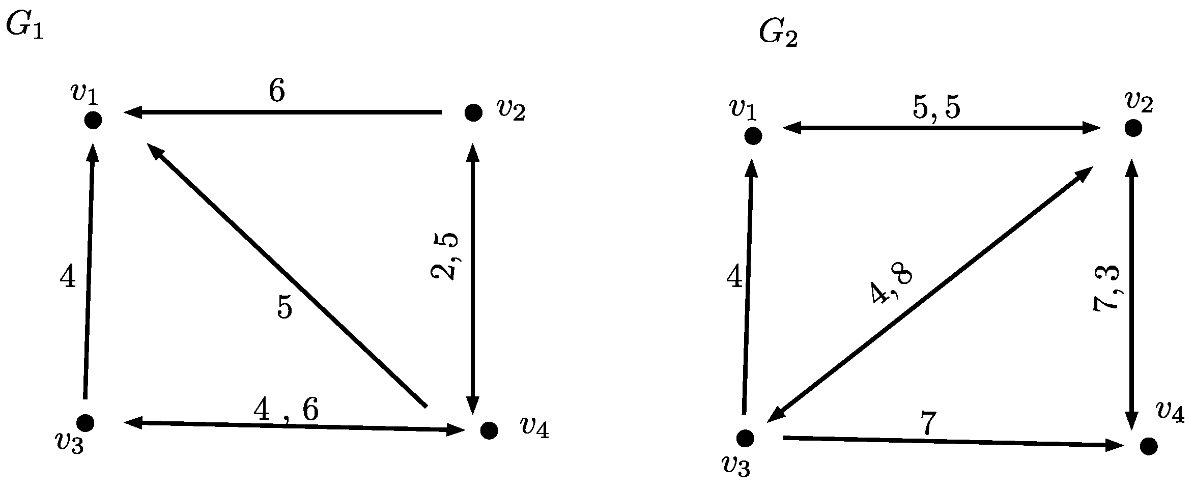
Given the two graphs $G_1$ and $G_2$ in Figure 1 and their respective adjacent matrices, in which the symbol ∞ (represented by a sufficient large real number) denotes there is no connection between the two nodes and represents a predetermined sufficiently large real number, in

Table 1. Adjacent Matrices for $G_1$ and $G_2$.

(a pair $\alpha ,\beta$ denote the weights of the directed edges $e_{ij}$ and $e_{ji}$, respectively, where $i<j$).

One obtains $E_1(v_1)=\left\{v_1\right\},E_1(v_2)=\{v_1,v_2,v_4\},E_1(v_3)=\{v_1,v_3,v_4\},E_1(v_4)=\{v_1,v_2,v_3,v_4\}$; moreover, one also obtains $E_2(v_1)=\{v_1,v_2\},$ $E_2(v_2)=\{v_1,v_2,v_3,v_4\},$ $E_2(v_3)=\{v_1,v_2,v_3,v_4\},$ $E_2(v_4)=\{v_2,v_4\}$. The representation of these graphs via partial functions could be demonstrated by

Table 2. Representing Directed Graphs via Partial Functions.

V	${\mathit{W}}_1(.)$	${\mathit{W}}_2(.)$
$v_1$	$\left\{(v_1,0)\right\}$	$\{(v_1,0),(v_2,5)\}$
$v_2$	$\{(v_1,6),(v_2,0),(v_4,2)\}$	$\{(v_1,5),(v_2,0),(v_3,4),(v_4,7)\}$
$v_3$	$\{(v_1,4),(v_3,0),(v_4,4)\}$	$\{(v_1,4),(v_2,8),(v_3,0),(v_4,7)\}$
$v_4$	$\{(v_1,5),(v_2,5),(v_3,6),(v_4,0)\}$	$\{(v_2,3),(v_4,0)\}$

.

By Equation (1), one has $d_1(G_1,G_2)=5+[|6-5|+|2-7|+4]+[|4-4|+|4-7|+8]+[5+6+|5-3|]=39.$ To simplify the whole computation, alternatively, this distance could also be obtained via the following matrix representation of Equation (1) and computation.

Definition 5.

$${\delta }_{ij}^n=\left\{\begin{array}{cc}1,\hfill & if{W}_n(i,j)\ne \infty ,\hfill \\ 0,\hfill & otherwise,\hfill \end{array}\right.$$

where $n\in \{1,2\}$.

Definition 6.

(distance between edges) Define each element $e_{ij}$ of the distance matrix $[W_1,W_2]$ between $W_1$ and $W_2$ by

$$e_{ij}={\delta }_{ij}^1·{\delta }_{ij}^2·|e_{ij}^1-e_{ij}^2|+(1-{\delta }_{ij}^1)·{\delta }_{ij}^2·e_{ij}^2+{\delta }_{ij}^1·(1-{\delta }_{ij}^2)·e_{ij}^1.$$

where $e_{ij}^1$ and $e_{ij}^2$ denote element of i’th row, j’th column in $W_1$ and $W_2$, respectively.

On the basis of this definition, one has

$$[W_1,W_2]=\left[\begin{array}{cccc}0& 5& 0& 0\\ 1& 0& 4& 5\\ 0& 8& 0& 3\\ 5& 2& 6& 0\end{array}\right].$$

Definition 7.

For any square matrix $S=(s_{ij})$, define ${\displaystyle ||S||=\sum _{i,j=1}^{|S|}{s}_{ij}}$.

Then, Equation (1) could be represented and computed via the following matrix operation:

$$d_1(G_1,G_2):=||[W_1,W_2]||=39.$$

5.2. Unlabelled Vertices with Singled Directed Edge

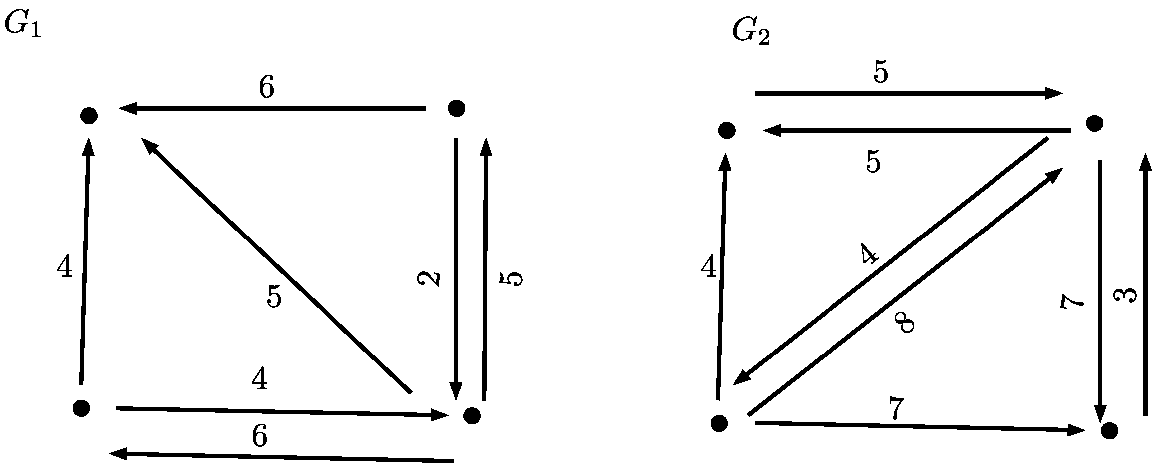
In this section, we show how to implement $d_2$ defined in Definition (4). Assume V is unlabelled. $G_1$ and $G_2$ are shown in Figure 2.

Let $N=\{v_1,v_2,v_3,v_4\}$ be the arbitrary names of the vertices of both $G_1$ and $G_2$. Let $PERM(n)$ denote all the permutations of the identity matrix with dimension n. By Equation (3), the distance between two unlabelled graphs could be represented and computed via the following matrix operations:

$$d_2(G_1,G_2):=min\{||[W_1,P^t{W}_{2}P]||:P\in PERM(|N|)\},$$

(5)

where each $P^t$ represents the transpose of the permutation matrix P. By computation, we have $|N|=4$, $|PERM(|N|)|=24$ and the distances between $W_1$ and each permutation of $W_2$ are listed as follows:

$$\begin{array}{c}\{||[W_1,P^t{W}_{2}P]||:P\in PERM(4)\}=\hfill \\ \{39,31,41,29,27,27,43,29,53,29,35,27,45,33,57,31,35,23,43,43,53,33,49,33\}.\hfill \end{array}$$

Among which, the optimal permutation matrix is $\overline{P}=\left[\begin{array}{cccc}0& 0& 1& 0\\ 0& 0& 0& 1\\ 0& 1& 0& 0\\ 1& 0& 0& 0\end{array}\right]$ and thus $d_2(G_1,G_2)=||[W_1,{\overline{P}}^t{W}_2\overline{P}]||=23,$ where ${\overline{P}}^t{W}_2\overline{P}=\left[\begin{array}{cccc}0& \infty & \infty & 3\\ 7& 0& 4& 8\\ \infty & \infty & 0& 5\\ 7& 4& 5& 0\end{array}\right]$. The corresponding minimal pair of graphs could be shown in Figure 3.

This could be interpreted as the complexity of the overlap of these two graphs based on corresponding vertices, i.e., this overlap yields the minimal complexity of the graphs.

6. Conclusions

In this article, we have shown how to define distances between graphs over either a set of labelled or unlabelled vertices via metrics $d_1$ and $d_2$, respectively. We also give a computational approaches to implement the computation of $d_1$ and $d_2$ via adjacent matrix operations. This implementation gives an efficient and fast computation of the distance between any two such graphs. This type of distance could then be applied in measuring the distance between networks or tree structures.

References

- Pawlak, Z. Rough Sets: Theoretical Aspects of Reasoning about Data; Kluwer Academic Publishers: Dordrecht, The Netherlands, 1991. [Google Scholar]
- Xu, C. Improvement of the distance between intuitionistic fuzzy sets and its applications. J. Intell. Fuzzy Syst. 2017, 33, 1563–1575. [Google Scholar] [CrossRef]
- Zadeh, L.A. Fuzzy Sets. Inf. Control 1965, 8, 338–353. [Google Scholar] [CrossRef]
- Liu, X. Entropy, distance measure and similarity measure of fuzzy sets and their relations. Fuzzy Sets Syst. 1992, 52, 305–318. [Google Scholar]
- Sarwar, M.; Akram, M. An algorithm for computing certain metrics in intuitionistic fuzzy graphs. J. Intell. Fuzzy Syst. 2016, 52, 2405–2416. [Google Scholar] [CrossRef]
- Akram, M.; Waseem, N. Certain Metrics in m-Polar Fuzzy Graphs. New Math. Nat. Comput. 2016, 12, 135–155. [Google Scholar] [CrossRef]
Figure 1.
Labelled graphs: and .
Figure 2.
Unlabelled graphs: and .
Figure 3.
Optimal pair of graphs: and .