2. Jacob’s Ladder
One can argue that prime numbers present perplexing features, somewhat of a hybrid of local unpredictability and global regular behavior. It is this interplay between randomness and regularity that motivated searches for local and global patterns that could perhaps be signatures of more fundamental mathematical properties.
Our work is concerned with the long standing question of the prime numbers distribution, or more precisely with the gaps between primes [
19,
20], a topic that has attracted much attention recently [
16,
21,
22] after some massive advances [
23]. Some problems related to prime gaps are well known, for instance, Legendre’s conjecture states that there is a prime number between
and
for every positive integer
n. This conjecture is one of Landau’s problems on prime numbers [
24] and, up to the current date (2018), it is still waiting to be proved or disproved. Another example would be the famous twin primes conjecture [
25]. Proving this conjecture seemed to be far out of reach until just recently. In 2013, Zhang demonstrated the existence of a finite bound
70,000,000, such that there are infinitely many pairs of distinct primes which differ by no more than
B [
23]. After such an important breakthrough, proving the twin prime conjecture looked much more plausible. Immediately after, a cooperative team led by Terence Tao, building upon Zhang’s techniques, was able to lower that bound down to 4680. Then, in the same year, Maynard slashed the value of
B down to 600, and finally the Polymath project further reduced it to 246 [
26,
27,
28].
Displaying numbers in two dimensions has been a traditional approach toward primes visualization [
29,
30]. Here, we propose an original way of number arrangement yielding an appealing visual structure: an oscillating plot that increases and decreases according to the prime number distribution. We plot the integers from 1 to
n in 2D (
x,
y) starting with 1 and
(hence, the first point will be (1, 0)), moving to 2 the plot moves up on the
y-axis, so that the next point in terms of coordinates is (2, 1). In the next step, it goes up or down depending on whether the number
n is a prime number or not. Number 2 is prime, so it flips in such a way that it goes down next, and hence the third point is (3, 0). Now, 3 is prime so the next step goes up again, and we move up to (4, 1). The number 4 is not a prime so it continues moving up, and so on. We used our own code but different codes to produce Jacob’s ladder can be found in the On-Line Encyclopedia of Integer Sequences [
31].
In
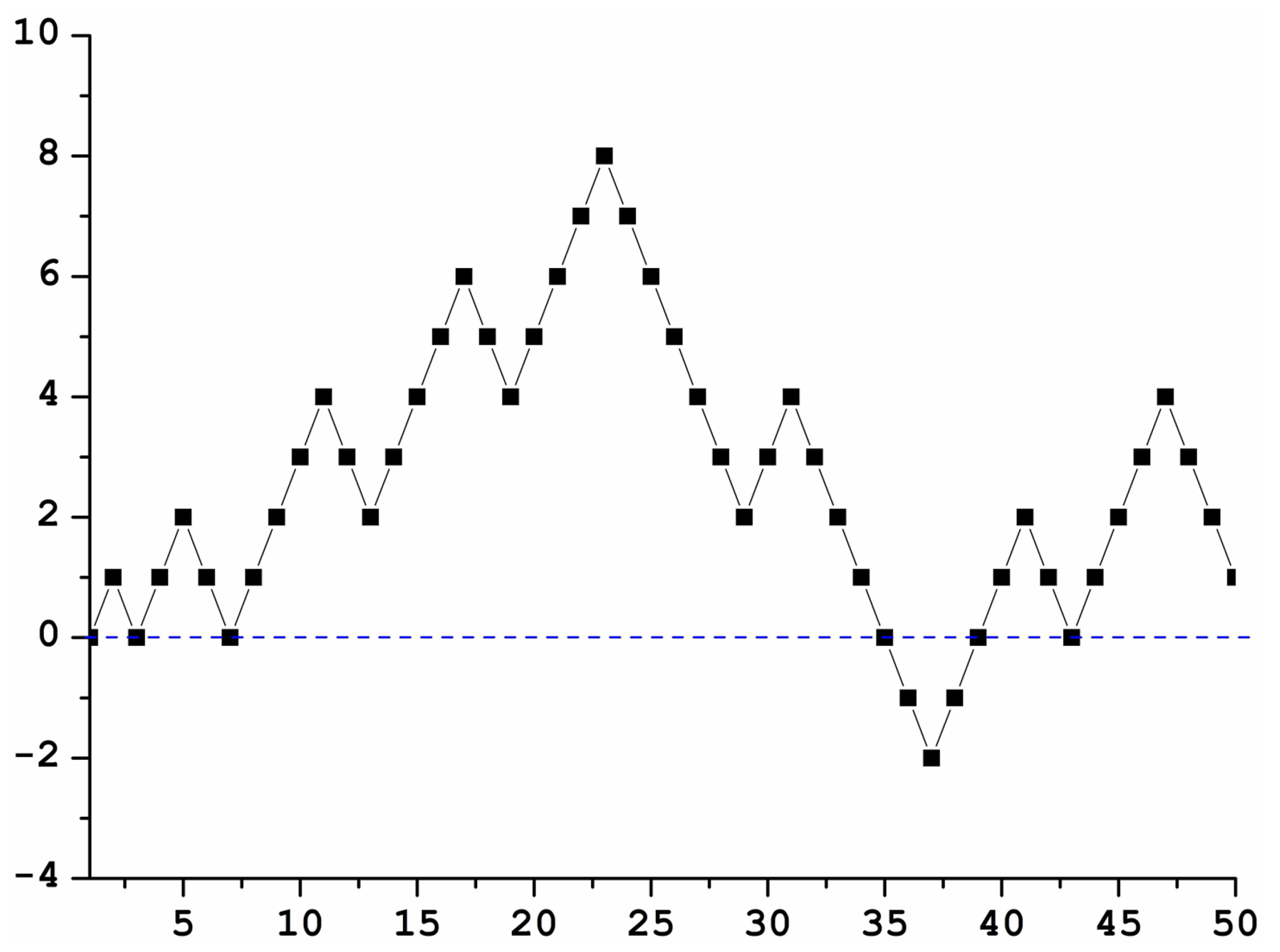
Figure 1, the sequence produced by the algorithm is shown up to
. The blue dashed line stands for the
line (or
x axis), which will be central to our study. We will refer to the points (
x, 0) as zeroes from now on. Because of the resemblance of this numerical structure to a ladder, we refer to this set of points in the 2D plane as
Jacob’s Ladder,
for short hereafter. The points in the ladder (the
y values) can be written as:
where
denotes the number of primes
.
3. Results
The next figures show the numerical results, which inspired the ideas and conjectures we will present in the next section.
Figure 2(Top) shows Jacob’s Ladder from 1 to 100. The blue dashed line signals the
x-axis for clarity’s sake. As can be seen, up to 100, the Ladder is almost positive, most of its points being above the
x-axis. This is misleading, though, as we can see from looking at the behavior of Jacob’s Ladder from 1 to 10,000 (
Figure 2(Bottom)).
Figure 2(Bottom) shows Jacob’s Ladder from 1 to 10,000. As can be seen, now most of the Ladder is negative except for two regions. However, this fact changes again if we move to higher values.
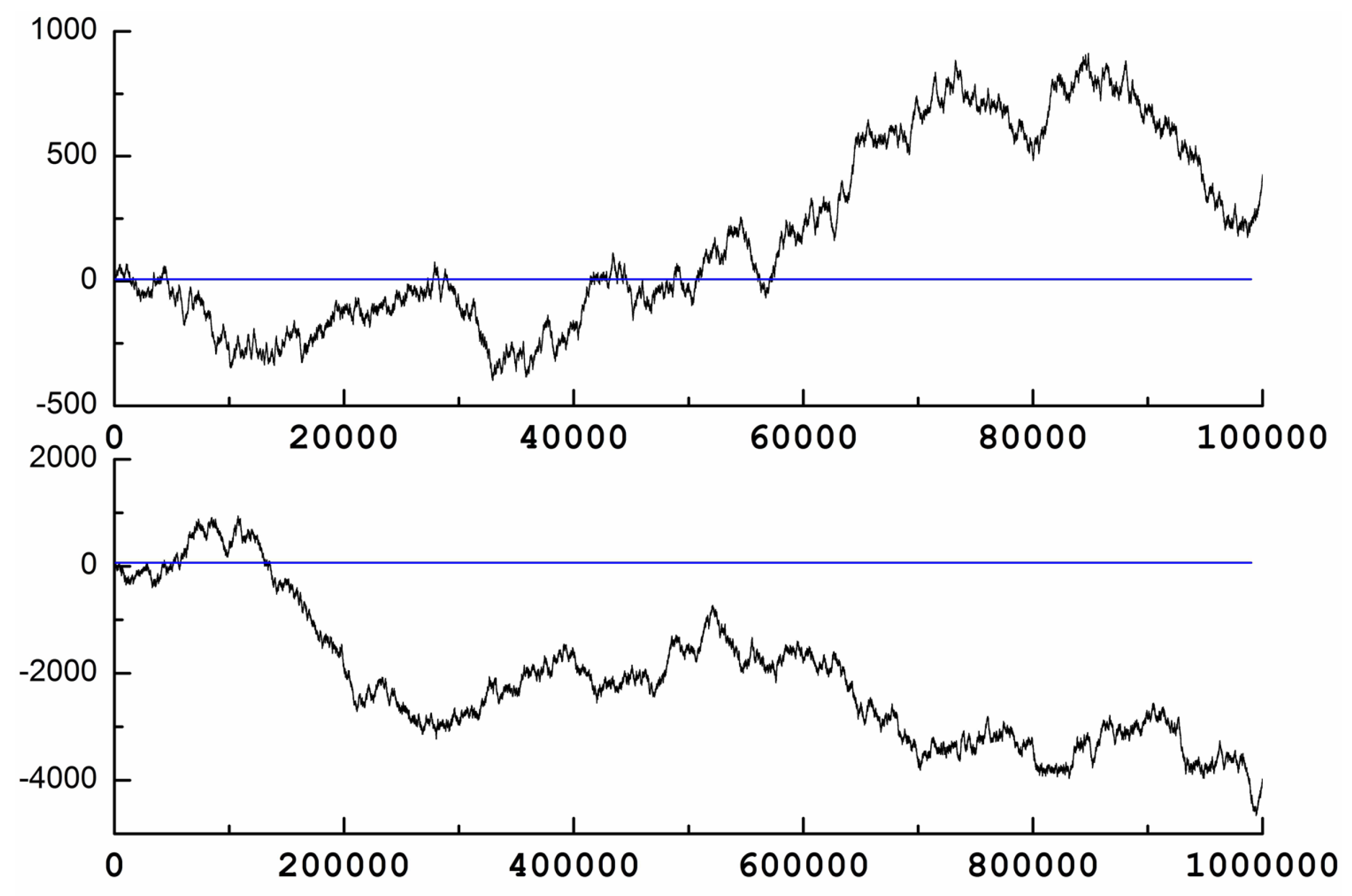
Figure 3(Top) shows Jacob’s Ladder from 1 to 100,000 and here we see, as said before, that, after
50,000, most of the Ladder is again positive.
Figure 3(Bottom) shows Jacob’s Ladder from 1 to 1,000,000. Note that the Ladder presents a big region of negative values after
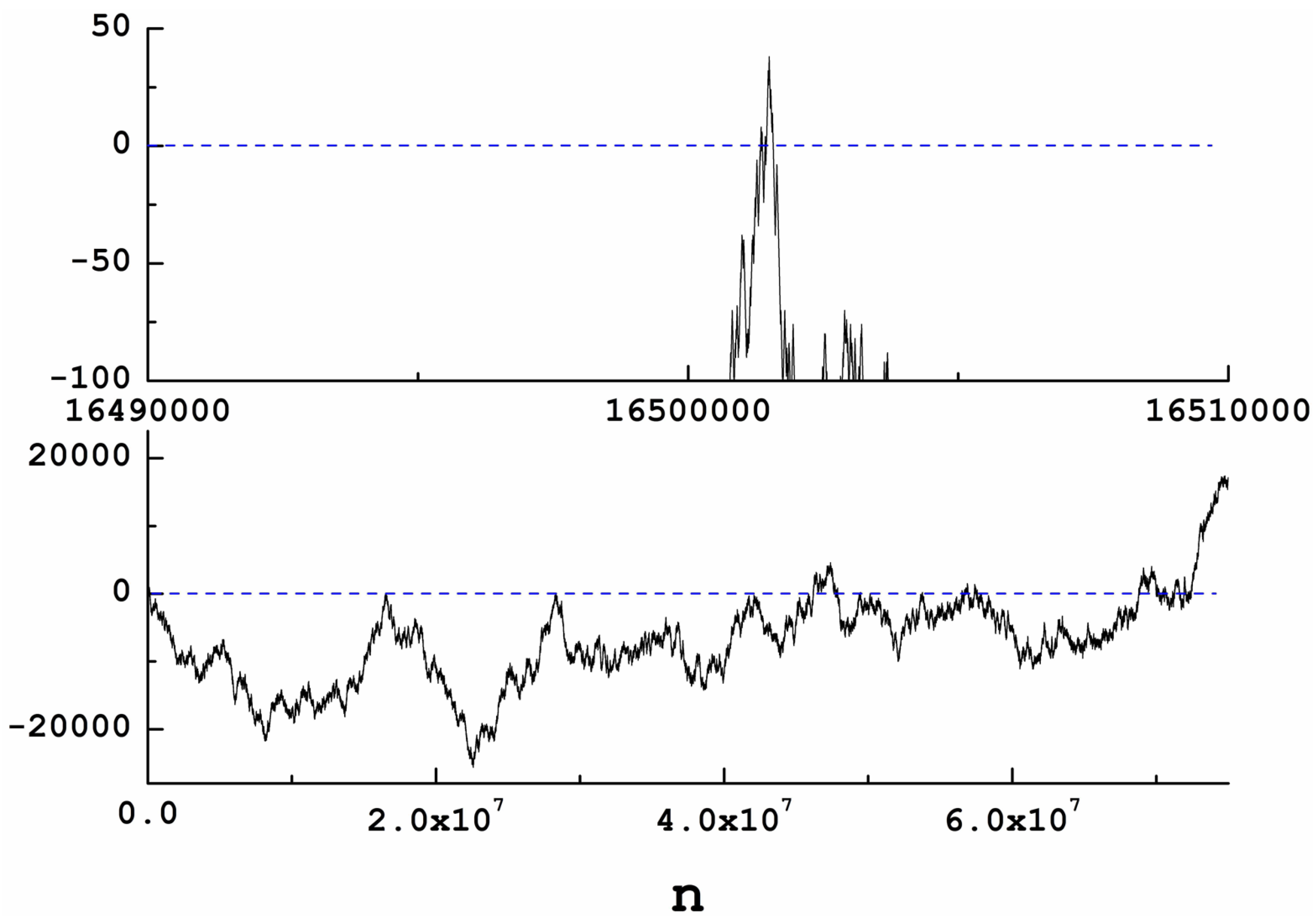
150,000. After this, no more zeroes are present up until 16,500,000 (see
Figure 4(Top)). Afterwards, the Ladder is mostly negative again.
Around 45 million, hundreds of zeroes are found (
Figure 4(Bottom)). Going up to 100 million, more zeroes appear, totaling 2415. The next crossing appears for
202,640,007. Larger gaps appear in the sequence at this point. For instance, no zeroes are found between 6,572,751,127 and 9,107,331,715.
Much larger is the gap found at 9,169,470,319. The next zero is 222,564,950,675. In addition, an even larger is the one from 225,888,362,295 to 676,924,242,679 (which are consecutive zeroes as well).
Jacob’s ladder resembles what in probability theory is called a Wiener process, so the probability distributions could be studied as well. It is quite clear that points very far from the x-axis will be less abundant when compared to the number of points close to it, above, or below the axis, so, renormalizing the number of points in the Ladder up to a given point, it seems natural to expect some version of an inverse arcsine law (centered around the x-axis) in the distribution of these points. Despite the large interval explored, the data are not enough to plot a convincing graph due to the ladder’s noticeable asymmetry, so we prefer to leave this point as an open question.
Building from the figures presented above, this simple representation of prime numbers in two dimensions brings about many interesting questions and allows us to arrive at a list of conjectures, which, despite their simplicity, will unfortunately be very difficult to prove or disprove. The most natural one is discussed below. Two additional ones are presented and analyzed in
Appendix A. The continuous appearance of an increasing number of zeroes, although sparse, points towards all of them holding true in the limit of large numbers.
Conjecture I:
The number of cuts (zeroes) on the
x-axis tends to infinity. In mathematical language,
being the number of zeroes in the Ladder,
Discussion:
Proving this conjecture is beyond the scope of this article, but, in the following, we describe the empirical motivation behind it. This is the main idea in our study and the basis of the conjectures that follow.
Figure 5 presents the number of zeroes vs.
n, in Jacob’s Ladder, from 1 to
(logarithmic scale on both axes). Notice that the number of zeroes increases (by construction, it cannot decrease) with
n in an apparently chaotic or unpredictable way. In some intervals of
n, the number of zeroes is constant, meaning that the ladder is entirely above or below
. After those plateaus, it increases again and again. If our conjecture is true, it will increase forever as we move towards increasingly bigger values of
n. However, we conjecture as well that the slope dictating this increase will be lower and lower as
n goes to infinity. The fact that the prime numbers become increasingly separated seems to indicate so: since the prime numbers are more and more separated, the ladder will present a smaller amount of zigzagging.
The sequence of cuts, or zeroes, can be denoted as and in the same way infinitely many successions can be defined: being the number of cuts on the line up to n, being the number of cuts in up to n, and so on. In other words, we conjecture that contains infinitely many elements, and, if Conjecture I is true, then it is likely that any other will contain infinitely many terms when n tends to infinity. Thus, the Ladder allows for non-trivially defining infinitely many successions with infinitely many terms (and without repetitions), whose cardinal will be and the sum of all of them is again .
It is to be noted that the ladder cannot be constrained between two y-values, since the gaps between primes can be arbitrarily large. A lower or upper limit could exist, but not both.
An interesting question can be formulated here: how does
grow? What would be a good approximation for the number of zeroes given a value of
n? The answer is not trivial, since the
function is neither multiplicative nor additive. In
Figure 5, we present two simple functions that operate as approximate upper and lower limits of the
function, namely
and
, represented by red lines. The number of zeroes is not strictly confined between these two curves; however, the agreement is fair enough for the purposes of this paper. We also plotted the counting function
in blue, for the sake of comparison.
The idea here is not to extract accurate upper and lower bounds with these functions, but to simply offer a qualitative approximation. The reason why such a qualitative conclusion is relevant lies on the geometrical insight that can be extracted from these simple approximations. If the numbers from 1 to
were to be plotted within a square (for instance forming a spiral, like in [
29]), then having approximately
n zeroes (or any other selection of numbers used as tracking mechanism) would mean that the amount of zeroes we have is approximately given by the length of the side of the square. In an analogous way, if we display the numbers from 1 to
within a cube of side
n, then the side of the cube would give us that information. Therefore, having a number of zeroes constrained between
and
seems to point towards some kind of fractality for the number of zeroes present in the sequence
.
4. Discussion
While completing this paper, we found similar studies, like those presented in [
32,
33,
34]. For instance, in [
34], a one-dimensional random walk (RW), where steps up and down are performed according to the occurrence of special primes (twins and cousins), was defined. If there are infinitely many twins and cousins (as suggested by the Hardy–Littlewood conjecture), then the RW defined there will continue to perform steps forever, in contrast to the RW considered in [
32] or [
33], where random walks were finite. In our case, we prefer not to talk about random walks since the distribution of primes, despite mysterious, is not random. On the other side, the idea of Jacob’s ladder is simple and beautiful given that, due to the infinitude of prime numbers, its intrinsic complexity and zigzagging must continue indefinitely. Now, its properties, by definition, depend both on the number of primes in a given interval and on the separation between them. It is known that the gaps between consecutive prime numbers cluster on multiples of 6. Because of this fact, 6 is sometimes called the jumping champion, and it is conjectured that it stays the champion all the way up to about
[
35,
36].
Beyond
, and until
, the jumping champion becomes 30 (
), and, beyond that point, the most frequent gap is 210 (
) [
36]. It is a natural conjecture that, after some large number, the jumping champion will be 2310 (
) and so on. Further interesting results on some statistical properties between gaps have been recently found [
37,
38]. However, all of the aforementioned numerical observations, despite revealing intriguing properties of the primes sequence, are not easily put into our problem in order to know whether or not the Ladder will have infinitely many zeroes or not. On the other side, according to Ares et al. [
39], the apparent regularities observed in some works [
34,
40,
41] reveal no structure in the sequence of primes, and that is precisely a consequence of its randomness [
42]. However, this is a controversial topic. Recent computational work points that “after appropriate rescaling, the statistics of spacings between adjacent prime numbers follows the Poisson distribution”. See [
43,
44] and references therein for more on the statistics of the gaps between consecutive prime numbers.
The question at hand is encapsulated by whether, after a given number, all turns in the Ladder will have an “order”. By order, we mean that
will go up (or down) after the next prime, and then down (or up) and so on but always keeping a property: that an “averaged” curve will continue asymptotically along one particular direction of the plane without ever going back to the
x-axis—or, in other words, is it possible that, after an unknown number
X, the sum of all intervals between primes “up” minus the sum of all intervals “down” (or the other way around) will be positive (or negative) for all possible
values as
?
where
(
) stands for the interval between two primes [
] which make the Ladder go up (down) (
Sensu stricto this could be true for a number
and the sum represented by Equation (
3) could be
(or
) without crossing the
x-axis because we start from some point up (or down) the axis.). This looks unlikely and would be some interesting order property if it turned out to be the case (and it would prove Conjecture I to be false). If so, it would be interesting to find that number
X distinctly.
This is related to the question of whether the zeroes are randomly distributed, or follow some kind of ordered distribution. For instance, do the terms in
follow Benford’s law [
45]? In many different natural datasets and mathematical sequences, the leading digit
d is found to be non-uniformly distributed as opposed to naive expectations (The leading digit of a number is its non-zero leftmost digit. For example, the leading digits of 2018 and 994,455 are 2 and 9, respectively). Instead, it presents a biased probability given by
where
. While this empirical law was indeed first discovered by the Canadian–American astronomer, applied mathematician and autodidactic polymath Simon Newcomb [
46] in 1881, it is popularly known as Benford’s law, and also as the law of anomalous numbers [
45]. Up to date, many mathematical sequences such as
and
[
47], binomial arrays
[
48], geometric sequences, or sequences generated by recurrence relations [
49,
50], to cite a few, have been proved to conform to Benford.
Figure 6 shows the proportion of the different leading digits found in the different intervals
, up to 194,531 zeroes, and the expected values according to Benford’s law. Note that intervals
have been chosen such that
, with
D a natural integer, in order to ensure an unbiased sample where all possible first digits are a priori equiprobable. With that in mind, however, the results for the interval
are also presented because the number of zeroes are many times more than those found up to
. Obviously, the curve is likely to change as more and more zeroes are counted (it changes when fewer zeroes are counted). A straightforward calculation demonstrates that, in the best of cases, one should count up to five (or six) times the current number of zeroes before having a distribution in fair agreement with Benford’s law. Note that, in order to obtain such a large amount of zeroes, according to
Figure 5, it is likely that one should explore the Ladder in a 25 (36) or 125 (216) times larger interval, i.e., up to
(
).
On the other hand, it is natural to assume that the distribution presented by will be the same for all values of y. Thus, while being aware that the numbers are still very small from a statistical point of view, the analysis of the terms in more crowded sequences can provide further evidence for the random distribution (or better said, non-Benford-like distribution) of for all y.
Another point to be noticed is that all of the zeroes can be written as . This is not a surprise—in fact, it can be easily proved that it must be this way: after 3, which is the first zero excluding 1, all zeroes must be separated by a number twice the sum of the number of gaps between primes (every pair of primes is separated by an even number); therefore, the gaps between zeroes will always be a multiple of 4.
For one more test about some possible unexpected non-random properties of the zeroes in the Ladder, we can check the number of zeroes ending in a given odd digit (since all the even ones will not be in ). Doing so, we observe that they change depending on the explored interval, so there is no clear evidence of any trend (The terms ending in 1, 3, 5, 7, and 9 amount to 38,835, 38,905, 38,799, 38,898, and 39,093, respectively, in the first 194,530 zeroes, thus showing a uniform distribution ( each). A linear fit () to the data (in probabilities, given as %) provides the following result: (0.04315) and (0.00751). The slope is small, and just twice the error of the linear fit, so it is quite unsafe to assume a trend on this).
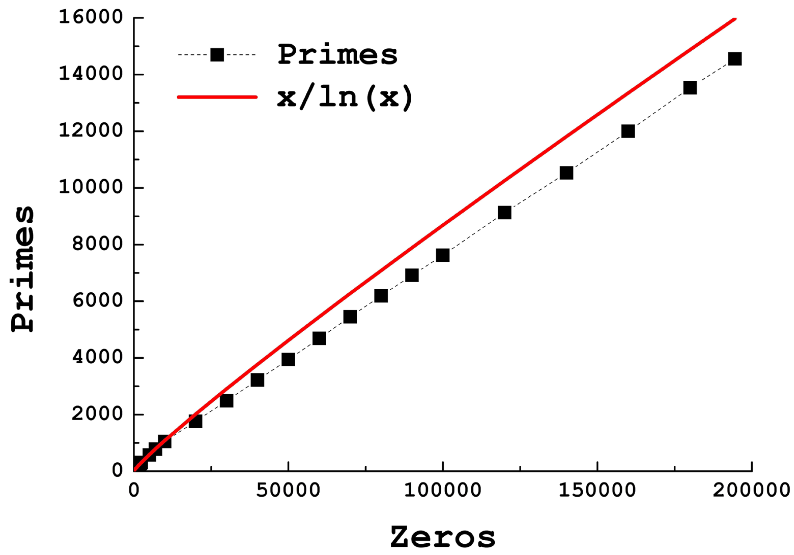
However, going back to the zeroes as a whole, we can observe the two most important results found in our study. First, it is natural to wonder: how many of these zeroes are primes? Is this number somewhere predictable? Since in an interval
we find
primes, should we expect, in a set of
X consecutive zeroes (but not consecutive numbers!), an amount of primes approximately equal to
? Interestingly, it seems to be the case if we count a few thousands of zeroes when looking at
Figure 7, but it is not really the case from looking at the differences in percentage (see
Table 1). The prime zeroes found are nevertheless in remarkable agreement with this simple assumption. As we see in
Figure 7, for
, the prime numbers found in
depart steadily from
, the latter being an overestimate of the actual number of primes.
As mentioned before, all zeroes can be written as
. However,
is the same as
. It is a well known result that all primes (except 2) can be written as
or
—the first ones allowing to be expressed as the sum of two perfect squares
, while the second ones can never be expressed in such a way. Therefore, in our results, those zeroes which are prime always belong to the second subgroup. Furthermore, the arithmetic progressions
, (and
) are of particular interest because the primes in the progression
(and
) are known to be “denser” than in the progression
(and
); a result conjectured in 1853 by Tschebyschef [
51,
52] and proved by Phragmen [
53] and Landau [
54]. However, the problem is, as is usually the case in number theory, far from being simple. A famous result by Littlewood [
2] showed that there are infinitely many integers
x such that there are more prime numbers in the progression
than in the
, up to that number
x (Using formal mathematical notation, it is said that
for infinitely many
x, where
denotes the number of positive primes
which are equal to c (mod b)).
It is easy to see that every sequence (or zeroes in the lines ) will contain primes (that is, reversals of the ladder) if and only if b is even. In particular, if , with a an integer number or zero, then those primes will belong to the arithmetic progression . In addition, those sequences where will contain primes belonging to the arithmetic progression (with the exception of 2, there are no primes in the sequences when b is odd). Thus, it is clear that the problem of how to demonstrate the existence of an infinite number of zeroes in Jacob’s Ladder is related with previous important results regarding primes in arithmetic progressions. However, it is not enough to know how many primes are found in a particular progression: the gaps between primes are equally important, and this is a more mysterious problem.
Now, we will see what can be said about gaps: how are the zeroes separated? As we have seen in
Figure 1,
Figure 2,
Figure 3 and
Figure 4, the Ladder goes up and down in an erratic way, resulting in a rather capricious distribution of the zeroes. Nevertheless, counting the number of times that a given gap between zeroes appears within a given number of zeroes, and the result is clearly non-arbitrary.
Figure 8 shows the result after analyzing the gaps in
up to
. It can be seen that a clear exponential decay is found. Note as well that all gaps are multiples of 4, except 2, which only appears once (The demonstration of the fact that all gaps are multiples of 4 is trivial).
The inset shows the averaged gap, , vs. the interval size. is calculated as the sum of gaps divided by the number of gaps. Another possible definition, , would be the interval size divided by the number of zeroes. The plateaus are due to intervals (from to for instance) where no more zeroes are found, so the number of gaps is constant. Using the definition, the averaged gap would be 10 times larger.
Figure 8, showing the distribution of gaps, is a remarkable result, and it may lead to a number of interesting observations. Note that almost 25% of the gaps are 4, 8, 12, or 16, and more than 53% of the gaps are smaller than 60. Gaps
represent more than 63% of the gaps found; however, as mentioned before, very large gaps are found as well as large as 451,035,880,384 (about half the interval explored).
In the intervals explored up to now, 4 is always the most frequent gap, referred to as hereafter, followed by , (i.e., the second most frequent gap is 8, the third most frequent is 12, etc.). Immediately, a legitimate and important question would be to inquire about the behavior of the distribution of gaps for large values of n. Will be 4 for any interval, no matter how large—or is it possible that, from a very large interval onwards, it shifts to 8, and later on to 12, and so on? Furthermore, it could be reasonable as well to expect an equiprobable distribution of gaps in the limit .
However, it has been shown that 4 is the most probable gap size (
Figure 8). If the exponential decay of
vs.
n hypothesis were finally confirmed
, such result would represent an attribute of the Ladder of fundamental importance, meaning that, every time that the ladder crosses the
x axis, it is close to a prime number. This observation can be misleading, though because, at the same time, the average gap clearly seems to increase with
n (Inset in
Figure 8). Thus, these results do not mean that all of the zeroes are primes. In fact, as showed before (See
Figure 7 and
Table 1), out of
n zeroes, about
are actually primes.
The percentage of gaps of length 4 decreases with
n faster than exponentially, in the same way as those of length 8 or 12, and likely for all gap values (in small intervals, some variations may occur, but we are interested in properties appearing in the limit of large intervals), as shown in
Figure 9. This result can be easily explained since, the larger the interval is, the more gaps enter into the list of gaps, so it is natural that the percentage would decrease.
At the same time, since the average gap increases, it could be natural to expect an increase in the percentage of larger gaps. However, this is not the case—only for small intervals do we observe an increase with n of the percentage of large gaps because, for small intervals, large gaps are rare, yet it seems that the percentage of large gaps is always below that of 4, 8, etc.
A final important remark: we started this work without knowing any previous studies on this topic—only while writing the paper did we check if the sequence of zeroes appeared in the On-Line Encyclopedia of Integer Sequences [
31], and then we found it was first studied in 2001 by Jason Earls and subsequently by Hans Havermann within a different context (See full sequence in
http://chesswanks.com/num/a064940.txt) and Don Reble (See full sequence in
https://oeis.org/A064940/a064940.txt).
