Prescribed Performance Adaptive Backstepping Control for Winding Segmented Permanent Magnet Linear Synchronous Motor


Abstract
:1. Introduction
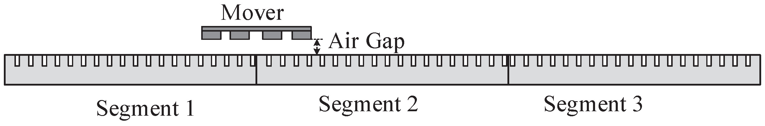
2. Mathematical Model of Winding Segmented Permanent Magnet Linear Synchronous Motor
Mathematical Model of PMLSMs
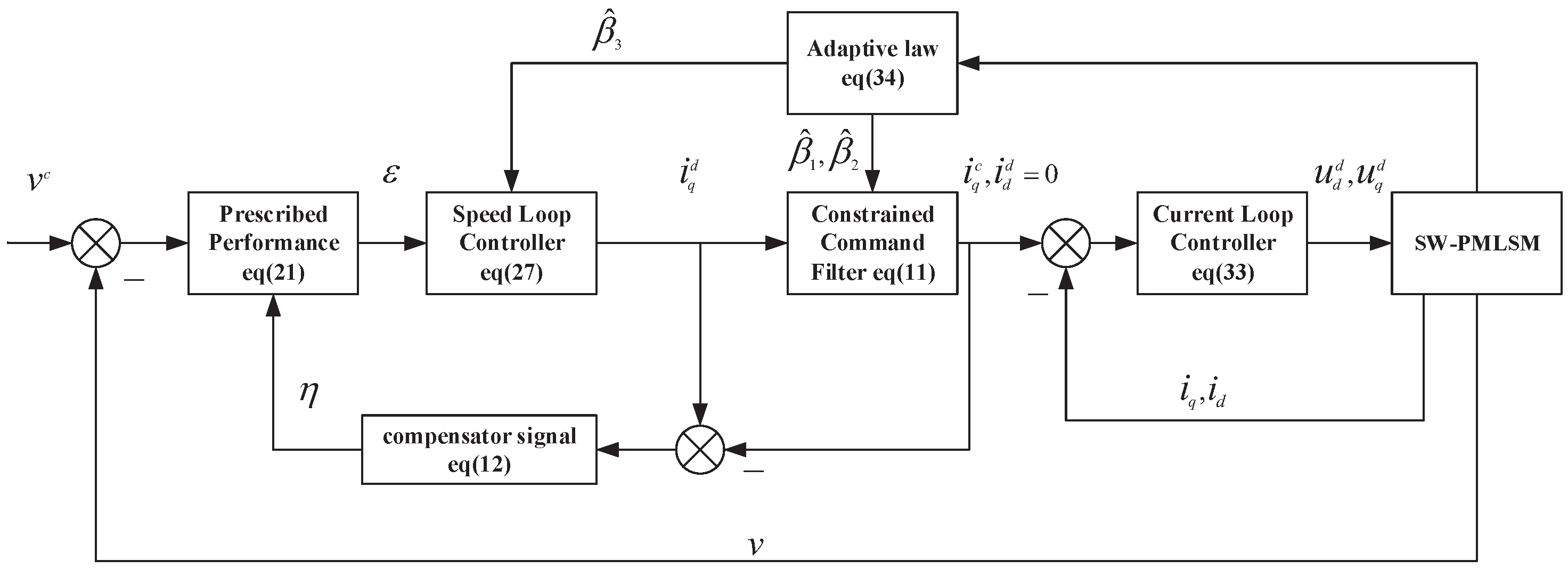
3. Prescribed Performance Adaptive Backstepping Controller Designer
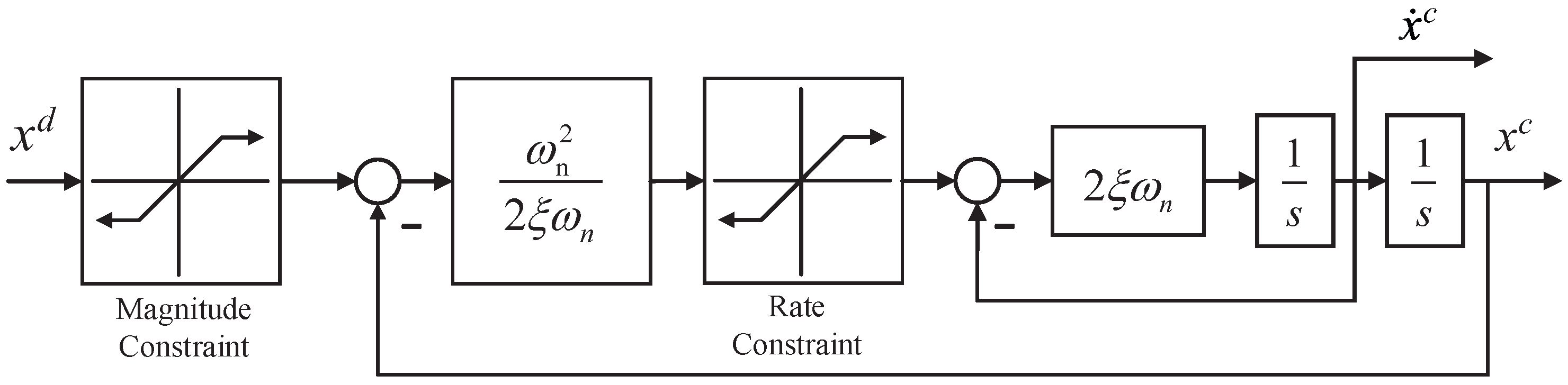
3.1. Constrained Command Filter
3.2. Prescribed Performance Function and Error Transformation
- 1.
- is positive and strictly decreasing.
- 2.
3.3. Prescribed Performance Adaptive Backstepping Controller Designer
3.4. Stability Analysis
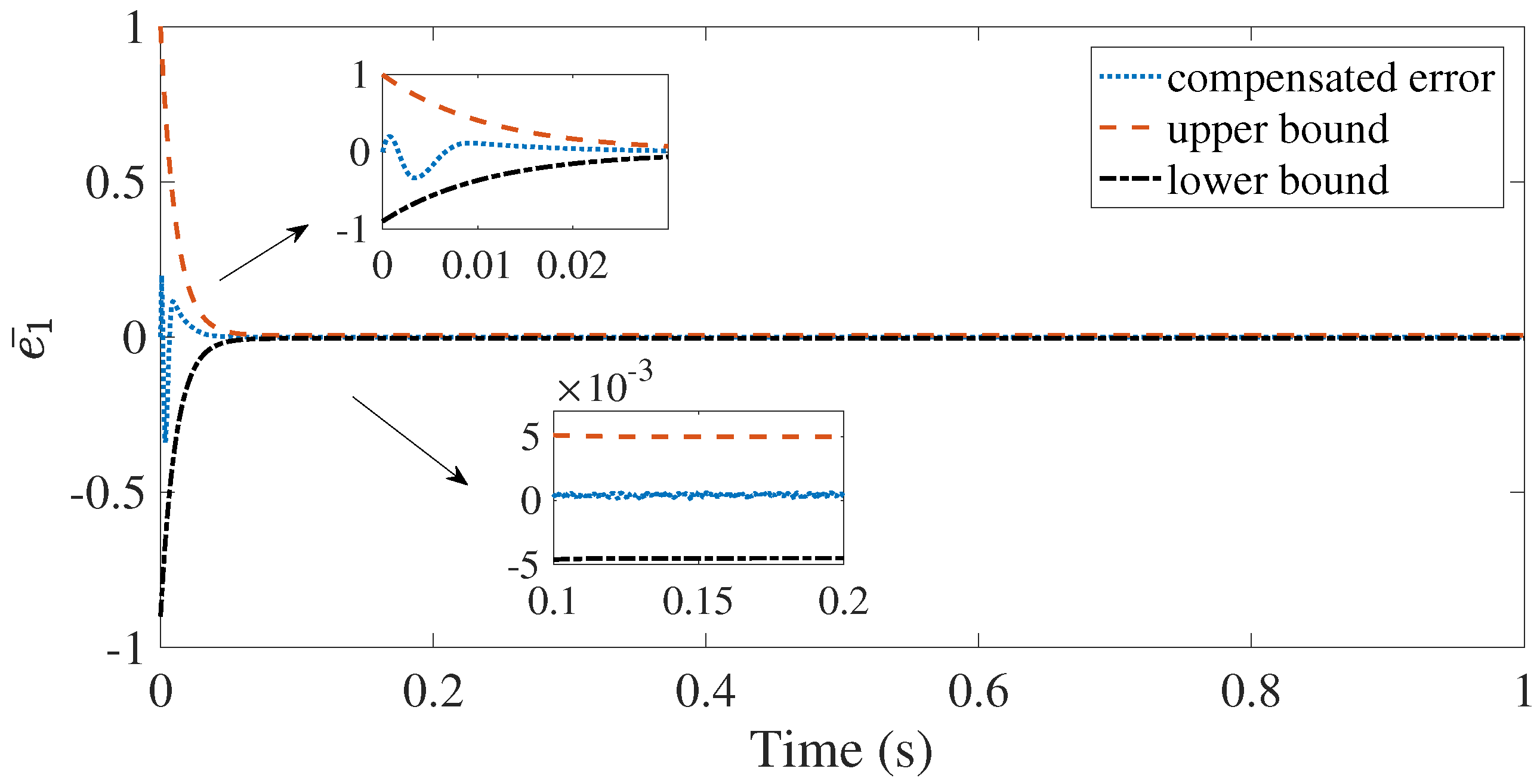
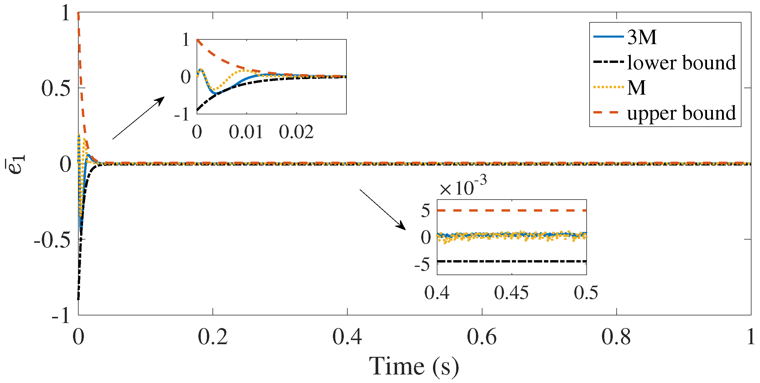
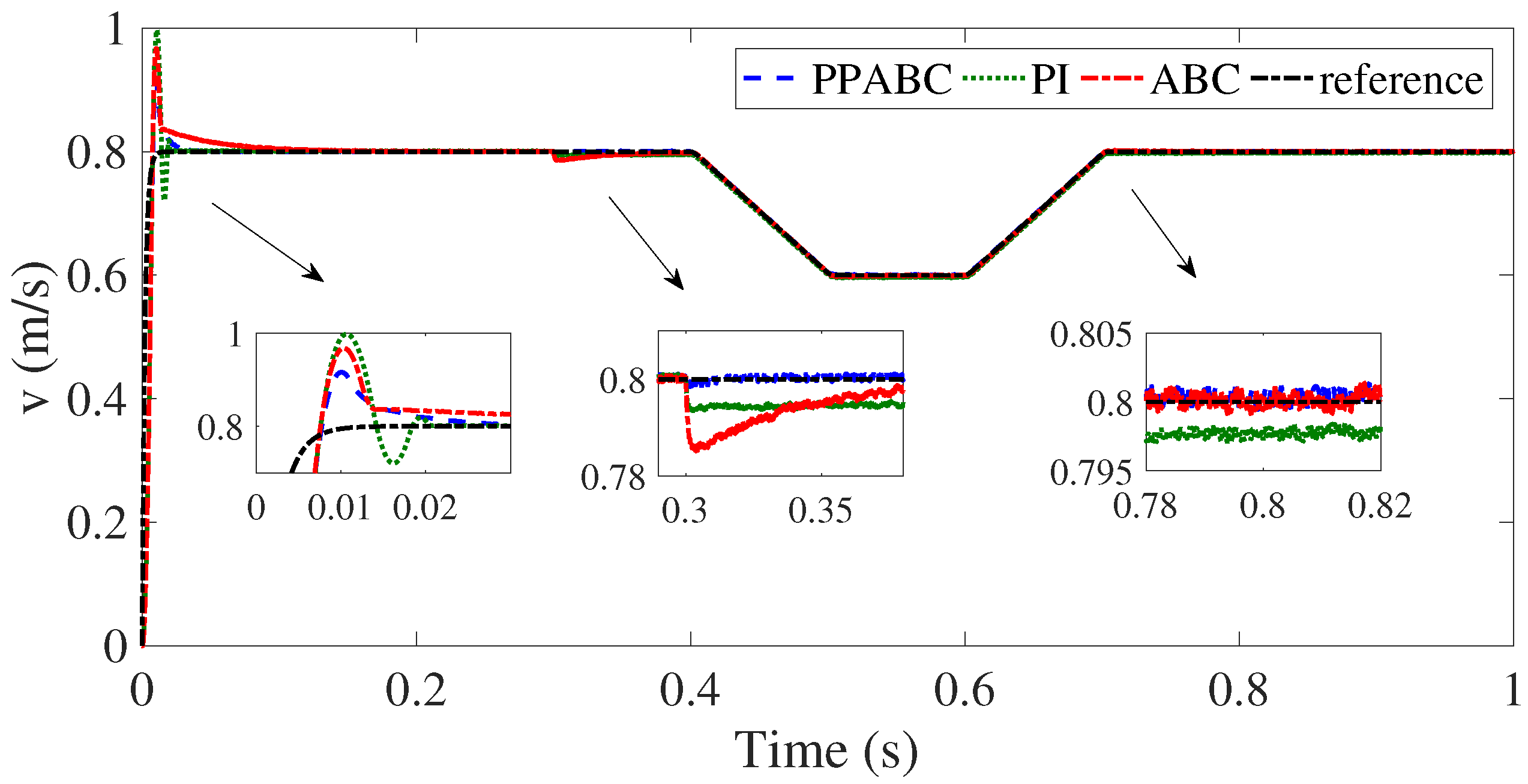
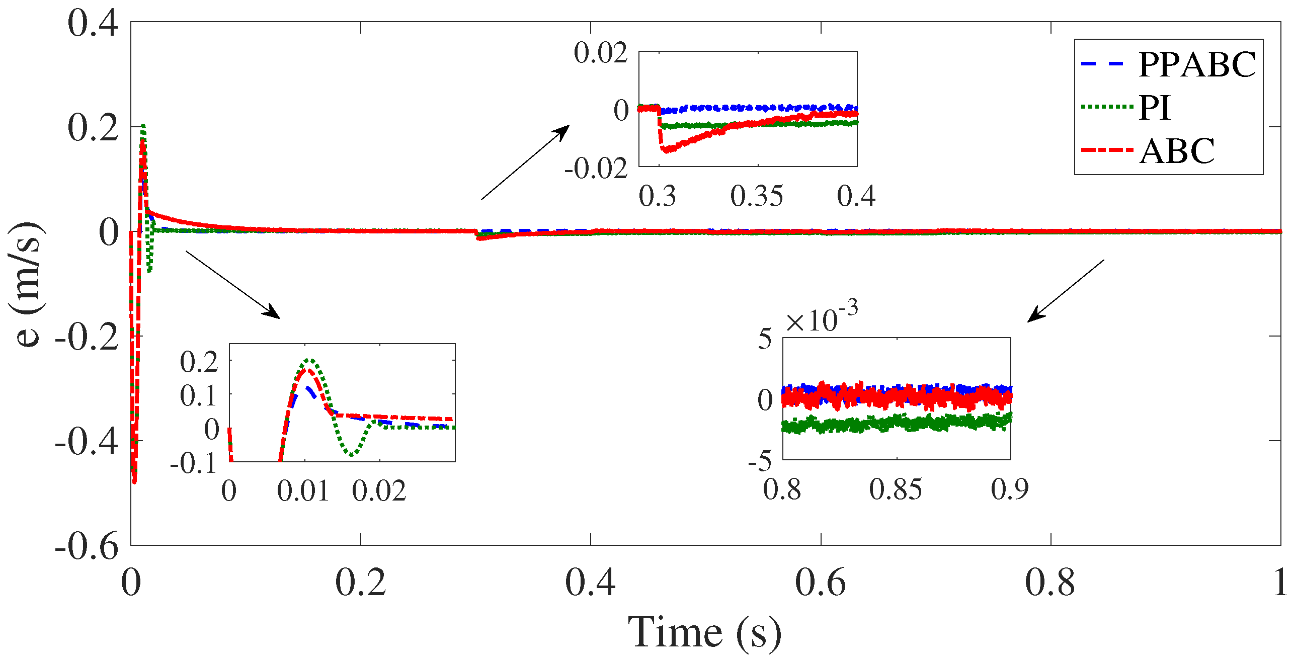
4. Simulation Study
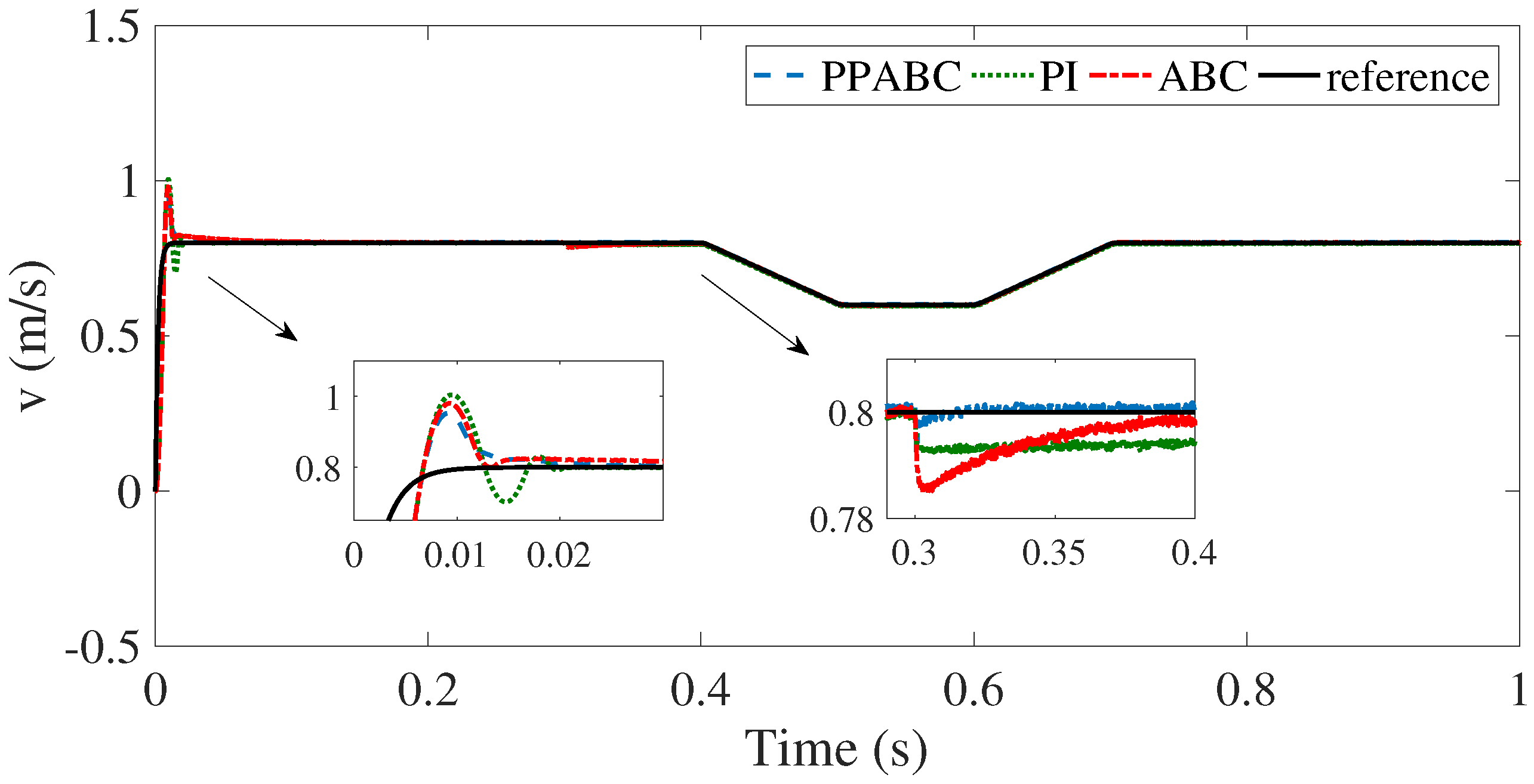
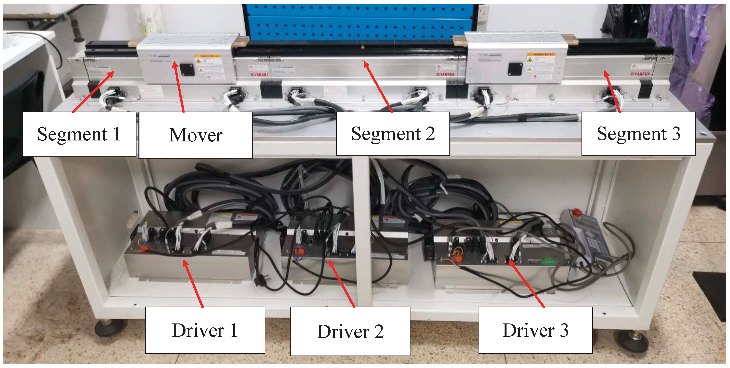
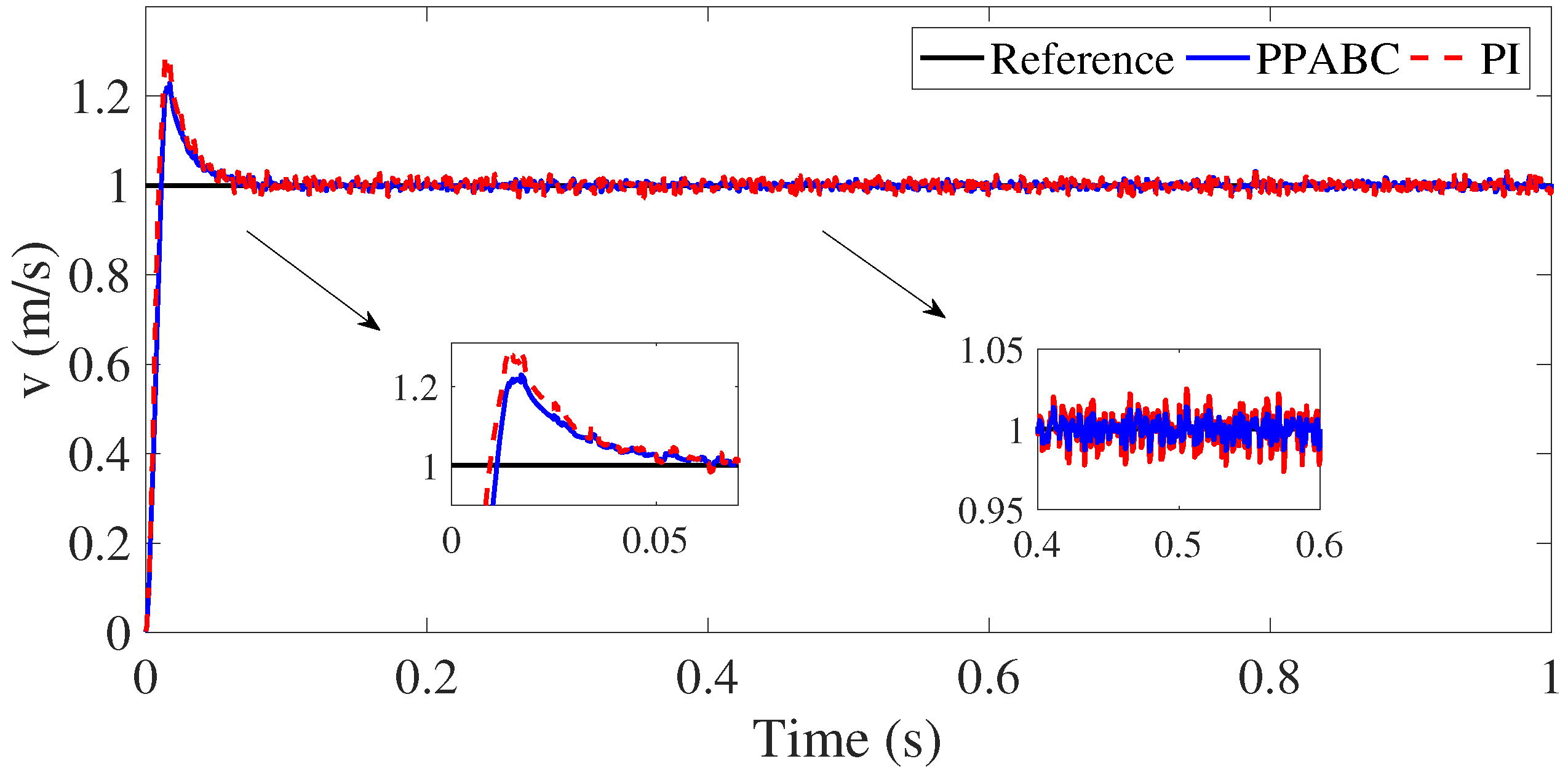
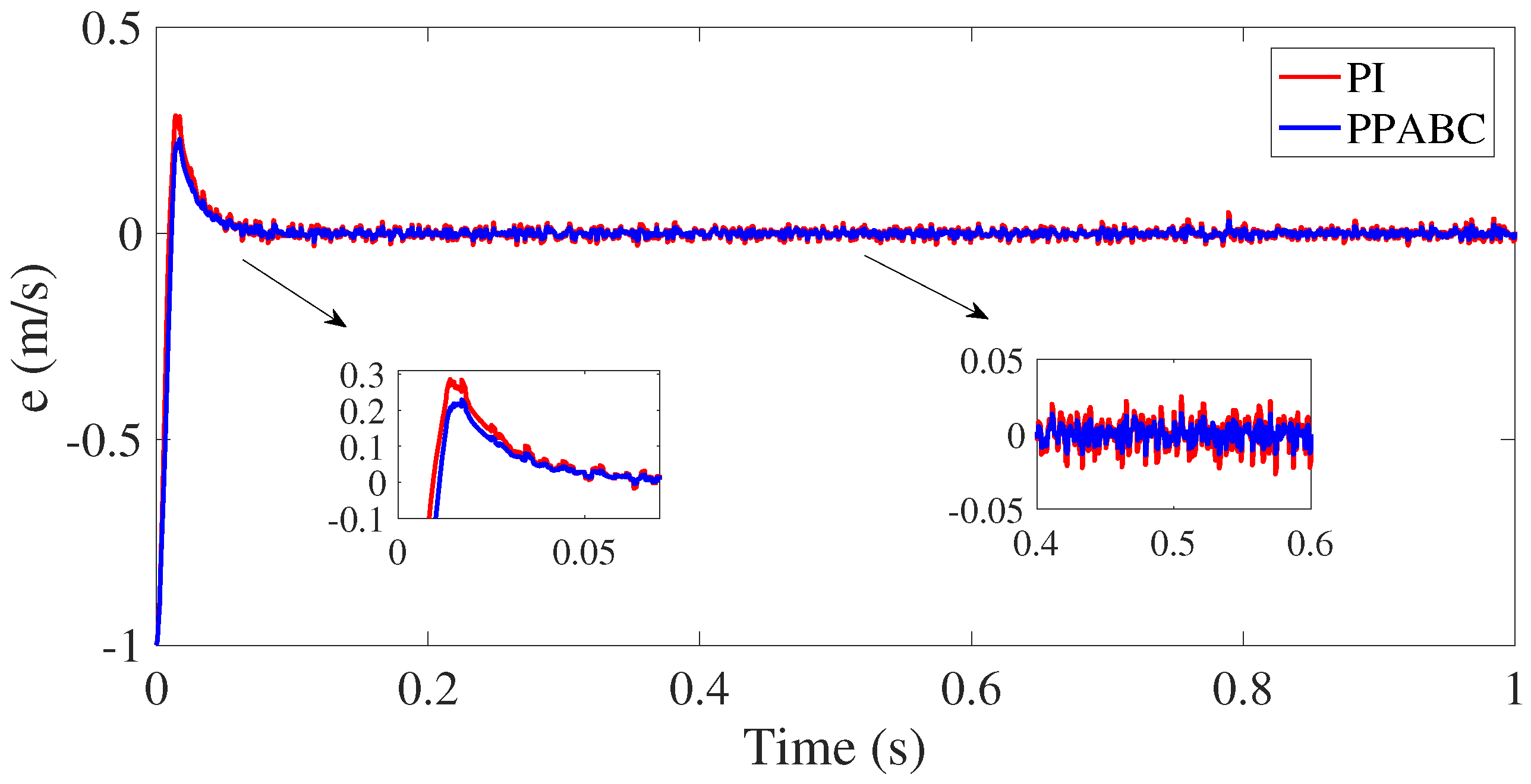
5. Experiment Validation
6. Conclusions
Author Contributions
Funding
Conflicts of Interest
References
- Li, X.; Du, R.; Denkena, B.; Imiela, J. Tool breakage monitoring using motor current signals for machine tools with linear motors. IEEE Trans. Ind. Electron. 2005, 52, 1403–1408. [Google Scholar] [CrossRef]
- Lin, F.J.; Shen, P.H.; Hsu, S.P. Adaptive backstepping sliding mode control for linear induction motor drive. IEE Proc. Electr. Power Appl. 2002, 149, 184–194. [Google Scholar] [CrossRef]
- Yoshida, K.; Nakata, S.; Koga, S. Orthogonally switching motion control of PMLSM vehicle in mass-reduced mode. In Proceedings of the Sixth International Conference on Electrical Machines and Systems, Beijing, China, 9–11 November 2003; pp. 469–472. [Google Scholar]
- Li, J.Q.; Li, W.L.; Deng, G.Q.; Ming, Z. Continuous-behavior and discrete-time combined control for linear induction motor-based urban rail transit. IEEE Trans. Magn. 2016, 52, 1–4. [Google Scholar] [CrossRef]
- Yue, F.; Li, X.; Chen, C.; Tan, W. Adaptive integral backstepping sliding mode control for opto-electronic tracking system based on modified LuGre friction model. Int. J. Syst. Sci. 2017, 48, 3374–3381. [Google Scholar] [CrossRef]
- Li, L.; Hong, J.; Lu, Z.; Ying, L.; Song, Y.; Liu, R.; Li, X. Fields and inductances of the sectioned permanent-magnet synchronous linear machine used in the EMALS. IEEE Trans. Plasma Sci. 2010, 39, 87–93. [Google Scholar] [CrossRef]
- Ma, M.N.; Li, L.Y.; Zhu, H.; Chan, C.C. Inductance and Flux Linkage Variation on Operation Performance for Multi-Segmented Linear PM Motor. Appl. Mech. Mater. 2013, 416, 15–20. [Google Scholar] [CrossRef]
- Li, L.; Hong, J.; Wu, H.; Zhao, Z.; Li, X. Adaptive back-stepping control for the sectioned permanent magnetic linear synchronous motor in vehicle transportation system. In Proceedings of the 2008 IEEE Vehicle Power and Propulsion Conference, Harbin, China, 3–5 September 2008. [Google Scholar]
- Hong, J.; Li, L.; Pan, D.; Zong, Z. Comparison of two current predictive control methods for a segment winding permanent magnet linear synchronous motor. In Proceedings of the 2012 16th International Symposium on Electromagnetic Launch Technology, Beijing, China, 15–19 May 2012. [Google Scholar]
- Hong, J.; Li, L.; Zong, Z.; Liu, Z. Current error vector based prediction control of the section winding permanent magnet linear synchronous motor. Energy Convers. Manag. 2011, 52, 3347–3355. [Google Scholar] [CrossRef]
- Chen, L.; Zhu, H.; Sun, S.G.; Li, Y.Y.; Zhu, L.G. Inter-Stator Synchronous Combined Method Based on SVM-DTC for Primary Winding Discontinuous PMLSM. Appl. Mech. Mater. 2014, 496, 1394–1400. [Google Scholar] [CrossRef]
- Zhao, W.; Jiao, S.; Chen, Q.; Xu, D.; Ji, J. Sensorless control of a linear permanent-magnet motor based on an improved disturbance observer. IEEE Trans. Ind. Electron. 2018, 65, 9291–9300. [Google Scholar] [CrossRef]
- Peng, C.C.; Li, Y.; Chen, C.L. A robust integral type backstepping controller design for control of uncertain nonlinear systems subject to disturbance. Int. J. Innov. Comput. Inf. Control 2011, 7, 2543–2560. [Google Scholar]
- Lin, F.J.; Hwang, J.C.; Chou, P.H. FPGA-based intelligent-complementary sliding-mode control for PMLSM servo-drive system. IEEE Trans. Power Electron. 2010, 25, 2573–2587. [Google Scholar] [CrossRef]
- Liu, H.; Pan, Y.; Li, S.; Chen, Y. Adaptive fuzzy backstepping control of fractional-order nonlinear systems. IEEE Trans. Syst. Man Cybern. Syst. 2017, 47, 2209–2217. [Google Scholar] [CrossRef]
- Hu, Q.; Shao, X.; Guo, L. Adaptive fault-tolerant attitude tracking control of spacecraft with prescribed performance. IEEE ASME Trans. Mechatron. 2017, 23, 331–341. [Google Scholar] [CrossRef]
- Yu, J.; Shi, P.; Dong, W.; Yu, H. Observer and command-filter-based adaptive fuzzy output feedback control of uncertain nonlinear systems. IEEE Trans. Ind. Electron. 2015, 62, 5962–5970. [Google Scholar] [CrossRef] [Green Version]
- Huang, P.; Wang, D.; Meng, Z.; Zhang, F.; Guo, J. Adaptive postcapture backstepping control for tumbling tethered space robot–target combination. J. Guid. Control Dyn. 2016, 39, 150–156. [Google Scholar] [CrossRef]
- Chen, C.P.; Wen, G.X.; Liu, Y.J.; Liu, Z. Observer-based adaptive backstepping consensus tracking control for high-order nonlinear semi-strict-feedback multiagent systems. IEEE Trans. Cybern. 2015, 46, 1591–1601. [Google Scholar] [CrossRef]
- Dhar, S.; Dash, P.K. Adaptive backstepping sliding mode control of a grid interactive PV-VSC system with LCL filter. Sustain. Energy Grids Netw. 2016, 6, 109–124. [Google Scholar] [CrossRef]
- Chen, F.; Jiang, R.; Zhang, K.; Jiang, B.; Tao, G. Robust backstepping sliding-mode control and observer-based fault estimation for a quadrotor UAV. IEEE Trans. Ind. Electron. 2016, 63, 5044–5056. [Google Scholar] [CrossRef]
- Xu, D.; Dai, Y.; Yang, C.; Yan, X. Adaptive fuzzy sliding mode command-filtered backstepping control for islanded PV microgrid with energy storage system. J. Frankl. Inst. 2019, 356, 1880–1898. [Google Scholar]
- Zhang, L.; Tong, S.; Li, Y. Dynamic surface error constrained adaptive fuzzy output-feedback control of uncertain nonlinear systems with unmodeled dynamics. Neurocomputing 2014, 143, 123–133. [Google Scholar] [CrossRef]
- Shen, Q.; Shi, P. Distributed command filtered backstepping consensus tracking control of nonlinear multiple-agent systems in strict-feedback form. Automatica 2015, 53, 120–124. [Google Scholar] [CrossRef]
- Sonneveldt, L.; Chu, Q.P.; Mulder, J.A. Nonlinear flight control design using constrained adaptive backstepping. J. Guid. Control Dyn. 2007, 30, 322–336. [Google Scholar] [CrossRef]
- Dong, W.; Farrell, J.A.; Polycarpou, M.M.; Djapic, V.; Sharma, M. Command filtered adaptive backstepping. IEEE Trans. Control Syst. Technol. 2011, 20, 566–580. [Google Scholar] [CrossRef]
- Li, Y.; Tong, S.; Liu, L.; Feng, G. Adaptive output-feedback control design with prescribed performance for switched nonlinear systems. Automatica 2017, 80, 225–231. [Google Scholar] [CrossRef]
- Li, Y.; Tong, S. Adaptive neural networks prescribed performance control design for switched interconnected uncertain nonlinear systems. IEEE Trans. Neural Netw. Learn. Syst. 2017, 29, 3059–3068. [Google Scholar] [CrossRef]
- Huang, Y.; Na, J.; Wu, X.; Liu, X.; Guo, Y. Adaptive control of nonlinear uncertain active suspension systems with prescribed performance. ISA Trans. 2015, 54, 145–155. [Google Scholar] [CrossRef]
- Yu, J.; Shi, P.; Zhao, L. Finite-time command filtered backstepping control for a class of nonlinear systems. Automatica 2018, 92, 173–180. [Google Scholar] [CrossRef]
- Hu, J.; Zhang, H. Immersion and invariance based command-filtered adaptive backstepping control of VTOL vehicles. Automatica 2013, 49, 2160–2167. [Google Scholar] [CrossRef]
- Wang, M.; Yang, A. Dynamic learning from adaptive neural control of robot manipulators with prescribed performance. IEEE Trans. Syst. Man Cybern. Syst. 2017, 47, 2244–2255. [Google Scholar] [CrossRef]
- Bechlioulis, C.P.; Rovithakis, G.A. Prescribed performance adaptive control for multi-input multi-output affine in the control nonlinear systems. IEEE Trans. Autom. Control 2010, 55, 1220–1226. [Google Scholar] [CrossRef]
- Rouche, N.; Habets, P.; Laloy, M. Stability Theory by Liapunov’s Direct Method; Springer-Verlag: New York, NY, USA, 1977. [Google Scholar]


| Definition | Parameter/Measure | Value |
|---|---|---|
| Mass | 3.5 | |
| Magnetic flux | 0.2 | |
| Friction coefficient | 0.027 | |
| Inductance | 0.1021 | |
| Resistance | 6.2689 | |
| Pole pitch | 0.027 | |
| Number of pole pairs | P | 2 |
© 2020 by the authors. Licensee MDPI, Basel, Switzerland. This article is an open access article distributed under the terms and conditions of the Creative Commons Attribution (CC BY) license (http://creativecommons.org/licenses/by/4.0/).
Share and Cite
Zhang, W.; Li, D.; Lou, X.; Xu, D. Prescribed Performance Adaptive Backstepping Control for Winding Segmented Permanent Magnet Linear Synchronous Motor. Math. Comput. Appl. 2020, 25, 18. https://doi.org/10.3390/mca25020018
Zhang W, Li D, Lou X, Xu D. Prescribed Performance Adaptive Backstepping Control for Winding Segmented Permanent Magnet Linear Synchronous Motor. Mathematical and Computational Applications. 2020; 25(2):18. https://doi.org/10.3390/mca25020018
Chicago/Turabian StyleZhang, Weiming, Dapan Li, Xuyang Lou, and Dezhi Xu. 2020. "Prescribed Performance Adaptive Backstepping Control for Winding Segmented Permanent Magnet Linear Synchronous Motor" Mathematical and Computational Applications 25, no. 2: 18. https://doi.org/10.3390/mca25020018