Article

A SARS-CoV-2 Fractional-Order Mathematical Model via the Modified Euler Method

1
Department of Mathematics, University of Malakand, Chakdara 18000, Khyber Pakhtunkhwa, Pakistan
2
Department of Mathematics and Computer Sciences, Faculty of Science, Necmettin Erbakan University, Konya 42090, Türkiye
3
Department of Mathematics, Art and Science Faculty, Siirt University, Siirt 56100, Türkiye
4
Mathematics Research Center, Department of Mathematics, Near East University, North Cyprus, Mersin 10, Nicosia 99138, Türkiye
*
Author to whom correspondence should be addressed.
Math. Comput. Appl. 2022, 27(5), 82; https://doi.org/10.3390/mca27050082
Submission received: 20 July 2022 / Revised: 13 September 2022 / Accepted: 22 September 2022 / Published: 26 September 2022

Abstract

:
This article develops a within-host viral kinetics model of SARS-CoV-2 under the Caputo fractional-order operator. We prove the results of the solution’s existence and uniqueness by using the Banach mapping contraction principle. Using the next-generation matrix method, we obtain the basic reproduction number. We analyze the model’s endemic and disease-free equilibrium points for local and global stability. Furthermore, we find approximate solutions for the non-linear fractional model using the Modified Euler Method (MEM). To support analytical findings, numerical simulations are carried out.

1. Introduction

COVID-19 caused by SARS-CoV-2 is a highly transmissible and pathogenic coronavirus that appeared in late 2019 and has posed a danger to both human health and public safety [1,2]. The World Health Organization (WHO) declared it an endemic because it killed and affected many worldwide, particularly in the USA and Europe, in a short period of time [3]. Clinical research has not yet produced a remedy that can completely eradicate the virus from the human body. However, the research remains ongoing. Many therapies (such as vaccination, monoclonal antibody therapy, and plasma therapy) have been developed by researchers who successfully treat early-stage diseases, including MERS-CoV, SARS-CoV, Ebola, HIV, and influenza-like viral diseases. Additionally, our body’s immune system responds well to infections or disorders. Throughout this uncontrollable condition, nearly all virus-infected regions were locked down, social gatherings were banned, and strict social distancing measures in all situations were implemented to control virus spread. Research worked to control the spread of this virus from different points of analysis such as microbiology [4,5], pathology [6,7], and applied mathematics [8].
In addition to biological and medical research, theoretical studies based on mathematical models may also be crucial to this anti-pandemic effort in analyzing the behavior of the outbreak that made it an epidemic, making decisions about how to stop its spread, and in comprehending patterns of virus transmission within hosts. Several mathematical models for COVID-19 have been formulated at an epidemiological level [6,9,10,11,12,13,14,15,16,17,18,19,20,21]. The replication cycle of the SARS-CoV-2 virus and its interactions with the innate and adaptive immune systems are only limited by research done at the within-host level [5,22,23]. Susceptible, infected, and removed (SIR) models are generally used for measles, rubella, and other infectious diseases to investigate the quick spread behavior of these infectious diseases [24]. A susceptible, exposed, infected, and removed (SEIR) model is comparable to the SIR model. The classes S, I, and R represent the number of populations in each partition at a specific point in time [25,26]. However, the incubation period is used in the SEIR model, so a specific incubation period for infectious diseases is more applicable [26,27]. The incubation period of SARS-CoV-2 is 1–14 days [28,29,30,31]. Different models have been developed to study the mechanism behind the spread of COVID-19 [32,33,34].
At the time of SARS-CoV-2 infection, macrophages are first targeted by SARS-CoV-2, and SARS-CoV-2 propagates to T cells afterwards. At this stage of the virus route, T cells are activated and further involve differentiation. In addition, T cells produce cytokines (INF- α ), IL-6, and IL-10) associated with the different types of a T cell. A large amount of cytokines provides a greater activation of the immune response to fight against the virus. Particularly, T cells, C D 4 + T cells, and C D 8 + T cells have been playing a significant antiviral role in the fight against pathogens. There is also a risk of mounting autoimmunity or devastating inflammation. C D 4 + T cells help the immune system of the body by generating virus-specific antibodies with the activation of T-dependent B cells. However, C D 8 + T cells can kill virally infected cells, as they are cytotoxic. In general, many C D 8 + T cells in the infected SARS-CoV-2 body are found in nearly 80% of the total infiltrative inflammatory cells in the interstitial pulmonary tract, which play a significant role in clearing CoVs. The loss of C D 4 + T cells is correlated with the reduced conscription of lymphocytes and neutralizing the production of antibodies and cytokines, resulting in severe immune-mediated interstitial pneumonitis and delayed SARS-CoV-2 lung clearance [34,35,36,37].
Researchers have shown that a long-lasting and persistent response of T cells to S and other structural proteins (including the proteins M and N), which provides the sufficient knowledge to draft the SARS vaccine by combining viral structural proteins. These vaccines may provide a robust, efficient, and long-term response to the virus by memory cells [36]. Clinical trials also show that a monoclinic antibody therapy is an effective treatment tool that responds well to SARS-CoV-2 [34].
Fractional calculus is often employed for epidemic models [38,39,40,41,42,43,44]. It has been shown that the fractional-order model outperforms the integer-order model in handling the modeling process since it has many other desirable characteristics, such as excellent fitting with real data. Furthermore, memory and heredity characteristics make it more effective in modeling and analyzing real-world problems. Numerous definitions or operators in the fractional calculus, such as Caputo, Riemann-Liouville, Atangana-Baleanu, and Caputo-Fabrizio derivative [45,46], are helpful in modeling epidemic diseases.
In our paper, we study a model of in-host viral kinetics that describes the response of SARS-CoV-2 to epithelial cells. Section 2 presents the formulation of the model, Section 3 describes preliminaries, Section 4 presents the uniqueness and existence of the solution to the proposed model, Section 5 presents the steady state points and the derivation of the primary reproduction ratio, Section 6 and Section 7 present local and global stability analyses, respectively, Section 8 presents the numerical solution algorithm, Section 9 shows graphical representations to support the logical result, and Section 10 concludes.

2. Mathematical Model

We consider the mathematical model [5,47] used to analyze the fractional model of the within-host viral kinetics of SARS-CoV-2.
E p ( t ) = δ ( E p ( 0 ) E p ( t ) ) γ E p ( t ) F ( t ) I p ( t ) = γ E p ( t ) F ( t ) β I p ( t ) F ( t ) = ρ I p ( t ) ω F ( t ) ,
with initial conditions
E p ( 0 ) > 0 , I p ( 0 ) 0 , and , F ( 0 ) 0 .
Here, the whole population is divided into three compartments: virus-free pulmonary epithelial cells, represented by E p ( t ) , virus-free cells, represented by F ( t ) , and virus-infected pulmonary epithelial cells, denoted by I p ( t ) . Here δ , β , and ω denote the death rate of uninfected pulmonary epithelial cells, infected pulmonary epithelial cells, and the virus, respectively. The production rate of the virus is denoted by ρ . In the model, the term E p ( 0 ) denotes the initial number of uninfected cells at time zero, and δ E p ( 0 ) shows a constant regeneration of uninfected epithelial cells.
Several researchers have taken into account fractional-order derivative (FOD) for modelling the infectious diseases [48,49,50]. We used FOD in the Caputo sense, because it gives better results than the classical order. Several FOD operators were developed, but the Caputo and the Riemann–Liouville FD operators are the most generally used due to their simplicity and similarities [38,39,51]. Other derivatives include Katugampola, Hadamard, Atangana-Baleanu, and Caputo–Fabrizio [52].
0 c D t α E p = δ α ( E p ( 0 ) E p ) γ α E p F 0 c D t α I p = γ α E p F β α I p 0 c D t α F = ρ α I p ω α F ,
with initial conditions
E p ( 0 ) = K 1 > 0 , I p ( 0 ) = K 2 0 , and , F ( 0 ) = K 3 0 .

3. Basic Definitions and Theorems

Definition 1.
The Caputo fractional derivative of order α of z : ( 0 , ) R is defined as
0 c D t α [ z ( t ) ] = 1 Γ ( K α ) 0 t t ζ K α 1 z ( K ) ( ζ ) d ζ ,
where α ( K 1 , K ] , K = [ α ] + 1 , and [ α ] represents the integer part of α.
Theorem 1
([49]). Let the equilibrium of the following non-autonomous fractional order system be z = 0 .
0 c D t α z ( t ) = f ( t , z ) , z ( t 0 ) = z 0 .
Let ψ R n be a domain containing z = 0 . Let U ( t , z ) : [ t 0 , ] × ψ R be a continuously differentiable function such that V 1 ( z ) U ( t , z ) V 2 ( z ) and
0 c D t α U ( t , z ) V 3 ( z ) , f o r t 0 , z ψ ,
where V 1 ( t , z ) , V 2 ( t , z ) and V 3 ( t , z ) are continuous non-negative definite functions on ψ , and U is a Lipschitz continuous function (LCF), so z = 0 is globally asymptotically stable.
Lemma 1
([39]). Let function z ( t ) R be continuously differentiable. It follows that, for any time t 0 ,
1 2 0 c D t α z 2 ( t ) 0 c D t α z ( t ) , α ( 0 , 1 ) .

4. Existences and Uniqueness

Firstly, we discuss the uniqueness and existence of the solution to the proposed model. Applying the fractional integral as ( 0 c D t α ) 0 c D t α ( H ( t ) ) . = H ( t ) H ( 0 ) to Equation (3), we obtain
E p ( t ) E p ( 0 ) = 1 Γ ( α ) 0 t ( 1 η ) α 1 ( δ α ( E p ( 0 ) E p ( t ) ) γ α E p ( t ) F ( t ) ) d η , I p ( t ) I p ( 0 ) = 1 Γ ( α ) 0 t ( 1 η ) α 1 ( γ α E p ( t ) F ( t ) β α I p ( t ) ) d η , F ( t ) F ( 0 ) = 1 Γ ( α ) 0 t ( 1 η ) α 1 ( ρ α I p ( t ) ω α F ( t ) ) d η .
Using the initial conditions, (5) becomes
E p ( t ) = K 1 1 Γ ( α ) 0 t ( t η ) α 1 ( δ α ( E p ( 0 ) E p ( η ) ) γ α E p ( η ) F ( η ) ) d η , I p ( t ) = K 2 1 Γ ( α ) 0 t ( t η ) α 1 ( γ α E p ( η ) F ( η ) β α I p ( η ) ) d η , F ( t ) = K 3 1 Γ ( α ) 0 t ( t η ) α 1 ( ρ α I p ( η ) ω α F ( η ) ) d η .
We define the kernels in System (6) as
Υ 1 t , E p , I p , F = ( δ α ( E p ( 0 ) E p ( t ) ) γ α E p ( t ) F ( t ) ) Υ 2 t , E p , I p , F = ( γ α E p ( t ) F ( t ) β α I p ( t ) ) Υ 3 t , E p , I p , F = ( ρ α I p ( t ) ω α F ( t ) ) .
Therefore, by using (7), the system (3) becomes
E p ( t ) = K 1 1 Γ ( α ) 0 t ( t η ) α 1 Υ 1 η , E p , I p , F d η , I p ( t ) = K 2 1 Γ ( α ) 0 t ( t η ) α 1 Υ 3 η , E p , I p , F d η , F ( t ) = K 3 1 Γ ( α ) 0 t ( t η ) α 1 Υ 3 η , E p , I p , F d η .
Theorem 2.
The kernels of System (3) satisfy the Lipschitz continuity if there are finite and positive scalar constants C i , i = 1 , 2 , 3 , such that C 1 = γ α max t [ 0 , t * ] F δ α 0 , C 2 = β α 0 and C 3 = ω α 0 .
Proof. 
By considering the kernels given in (3), we have
Υ 1 t , E p , I p , F Υ 2 t , E p * , I p , F = δ α ( E p E p ( 0 ) ) γ α E p F δ α ( E p * E * ( 0 ) ) γ α E * F = γ α F E p E p * δ α E p ( 0 ) E * ( 0 ) ) + ( E p E p * γ α F δ α E p E p * γ α F δ α E p E p * γ α max t [ 0 , t * ] F δ α E p E p * C 1 E p E p * , C 1 = γ α max t [ 0 , t * ] F δ α ,
Υ 1 t , E p , I p , F Υ 2 t , E p , I p * , F = γ α E p F β α I p γ α E F β α I p * = β α I p * I p β α I p * I p C 2 I p * I p , C 2 = β α ,
Υ 1 t , E p , I p , F Υ 2 t , E p , I p , F * = ρ α I p ω α F ρ α I p ω α F * = ω α F * F ω α F * F ( t ) C 3 F * F , C 3 = ω α .
Hence, the proposed system satisfies the Lipschitz continuity. This means that the system is continuous and bounded. □
Theorem 3.
Let α ( 0 , 1 ) , J = [ 0 , t * ] R and l = E p ( t ) E p * ( t ) A 1 . Let the function Υ 1 : j × l R be continuous and bounded. M > 0 such that Υ 1 t , E p , I p , F M 1 . We assume that v 1 satisfies the Lipschitz conditions. If C 1 A 1 < M 1 , then there is a unique Υ 1 t , E p , I p , F C [ 0 , t * ] , such that t * = m i n t , ( A 1 Γ ( α + 1 ) M 1 ) .
Proof. 
If F = E b C ( 0 , t * ) : E b ( t ) E b ( 0 ) A 1 , then F is a complete metric space since F R , and it is also a closed set. We now define the operator T in F as
T E p ( t ) = E p ( 0 ) + 1 Γ ( α ) 0 t ( t η ) α 1 Υ 1 η , E p , I p , F d η .
We then have
T E p ( t ) E p ( 0 ) = 1 Γ ( α ) 0 t ( t η ) α 1 Υ 1 η , E p , I p , F d η 1 Γ ( α ) 0 t ( t η ) α 1 Υ 1 η , E p , I p , F d η 1 Γ ( α ) 0 t ( t η ) α 1 M 1 d η = M 1 Γ ( α + 1 ) t α M 1 Γ ( α + 1 ) ( t * ) α M 1 Γ ( α + 1 ) A 1 Γ ( α + 1 ) M 1 ) = A 1 .
Hence,
T E p ( t ) E p ( 0 ) A 1 .
Similarly, we easily show that
T I p I p ( 0 ) A 2 ,
and
T F F ( 0 ) A 3 .
Finally, we need to show that T satisfies the contraction mapping theorem.
T E p T E p * ( t ) = E p ( 0 ) E p * ( 0 ) + 1 Γ ( α ) 0 t ( t η ) α 1 Υ 1 η , E p ( η ) , I p ( η ) , F ( η ) Υ 1 η , E p * ( η ) , I p ( η ) , F ( η ) d η .
Assuming that E p ( 0 ) = E p * ( 0 ) ,
T E p T E p * ( t ) = 1 Γ ( α ) 0 t ( t η ) α 1 Υ 1 η , E p ( η ) , I p ( η ) , F ( η ) Υ 1 η , E p * ( η ) , I p ( η ) , F ( η ) d η ,
which implies that
T E p T E p * 1 Γ ( α ) 0 t ( t η ) α 1 Υ 1 η , E p ( η ) , I p ( η ) , F ( η ) Υ 1 η , E p * ( η ) , I p ( η ) , F ( η ) d η .
By using the value of | ( Υ 1 ( η , E p ( η ) , I p ( η ) , F ( η ) ) Υ 1 ( η , E p * ( η ) , I p ( η ) , F ( η ) ) | d η , we obtain
T E p T E p * 1 Γ ( α ) 0 t ( t η ) α 1 C 1 E p * E p d η C 1 Γ ( α ) E p * E p 0 t ( t η ) α 1 d η C 1 Γ ( α + 1 ) E p * E p t α C 1 Γ ( α + 1 ) E p * E p ( t * ) α C 1 Γ ( α + 1 ) E p * E p A 1 Γ ( α + 1 ) M 1 .
Hence,
T E p T E p * ( t ) A 1 C 1 M 1 E p * E p .
Since A 1 C 1 M 1 < 1 , one can conclude that T satisfies the contraction mapping theorem and it has a unique fixed point.
In the same procedure, we obtain
T I p T I p * A 2 C 2 M 2 I p * I p .
T F T F * A 3 C 3 M 3 F * F .
Thus, System (3) has a unique solution. □

5. Steady State and Derivation of Reproduction Number R 0

Let E 0 be the disease-free equilibrium point, and from the equations in (3), we set the right-hand sides as equal to zero and solve for variables.
δ α ( E p E p ( 0 ) ) γ α E p F = 0 ,
γ α E p F β α I p = 0 ,
ρ α I p ω α F = 0 .
If I p and F are equal to zero, we obtain the disease-free equilibrium as
E 0 = E p 0 , I p 0 , F 0 = E p ( 0 ) , 0 , 0 .
To find the endemic equilibrium E * = E p * , I p * , F * , we consider E p ( t ) 0 , I p ( t ) 0 , in Equations (13)–(15) as
E p * = 1 δ α β α I p * E p ( 0 ) ,
I p * = γ α β α δ α β α ω α ρ α F * E p ( 0 ) F * ,
F * = ω α ρ α I * .
Next, we want to derive the reproduction number R 0 . The reproduction number is a threshold quantity representing the total number of secondary illnesses caused by an infected individual in a fully susceptible population throughout the infectious period [53].
For this, we develop the next generation matrix approach. Let M ( S ) represent the rate of new infections, and let X ( S ) represent the transfer rate of individual. We then have M ( S ) = γ α E p ( t ) F ( t ) 0 and X ( S ) = β α I p ρ α I p ω α F .
The Jacobian matrices J M ( S ) and J X ( S ) at the non-infected steady state (16) are
m = J M ( S ) = 0 γ α E p ( 0 ) 0 0 , x = J X ( S ) = β α 0 ρ α ω α .
x 1 = 1 ω α β α ω α 0 ρ α β α .
m x 1 = 1 ω α β α 0 γ α E p ( 0 ) 0 0 ω α 0 ρ α β α = ρ α γ α E p ( 0 ) ω α β α β α γ α E p ( 0 ) ω α β α 0 0 .
The reproduction number is given by the spectral radius of the next generation matrix m x 1 . We then obtain λ 1 = 0 , λ 2 = ρ α γ α E p ( 0 ) λ α β α , from the absolute highest eigenvalues from m x 1 . Thus, from the model (3), we obtain the expression for R 0 as
R 0 = ρ α γ α E p ( 0 ) λ α β α .
The following graphical representation describes the potential impact of introducing a new SARS-CoV-2 variant with high transmission rates. Figure 1 represents the effects of the basic reproduction number with respect to different parameters.

6. Local Stability

In this part of the paper, we discuss the local stability of the steady-state point (16). For this need, we write the Jacobian matrix for the system (3) as
J = δ α γ α F 0 γ α E p γ α F β α γ α E p 0 ρ α ω α .
Theorem 4.
The non-infected steady state E 0 is locally asymptotically stable when R 0 < 1 .
Proof. 
The Jacobian matrix for the steady state (16) as □
J ( E 0 ) = δ α 0 γ α E p ( 0 ) 0 β α γ α E p ( 0 ) 0 ρ α ω α .
According to the Routh–Hurwitz criteria [54], if all the real parts of the value of the real eigenvalues of the Jacobian matrix are negative, then E 0 is locally asymptotically stable. In order to show that, we have
λ I J E 0 = δ α λ 0 γ α E p ( 0 ) 0 β α λ γ α E p ( 0 ) 0 ρ α ω α λ = 0 .
The characteristics equation of the above matrix is
δ α λ λ 2 + λ ( ω α + β α ) + β α ω α ρ α γ α E p ( 0 ) = 0 ,
δ α λ λ 2 + a 1 λ + a 2 = 0 ,
with a 1 = ω α + β α , and a 2 = β α ω α ρ α γ α E p ( 0 ) .
Based on an equation, the eigenvalues λ 1 = δ α > 0 , and a 1 = ω α + β α > 0 were obtained. According to Routh–Hurwitz stability criteria, a 2 = β α ω α ρ α γ α E p ( 0 ) > 0 β α ω α > ρ α γ α E p ( 0 ) 1 > ρ α γ α E p ( 0 ) β α ω α R 0 < 1 .
Therefore, if R 0 < 1 , then all the conditions of Routh–Hurwitz criteria are satisfied. Hence, the non-infected steady-state E 0 becomes locally asymptotically stable if R 0 < 1 and unstable if R 0 > 1 .

7. Global Stability

In this part of the paper, we use the Lyapunov function approach to investigate the result for the model’s globally asymptotically stability (GAS) in the disease-free state. For this, we have the following theorem.
Theorem 5.
When R 0 < 1 , the disease-free equilibrium E 0 is globally asymptotically stable; otherwise, it is unstable.
Proof. 
For this, we derive the Lyapunov candidate function (LCF) for the fractional-order as in [38]. We then take the family of the Lyapunov function
L ( e 1 , e 2 , . . . , e n ) = i = 1 n p i 2 e i ( t ) e * 2 .
LCF is defined as
L E p , I p , F = 1 2 E p E p * 2 + 1 2 I p I p * 2 + 1 2 F p F p * 2 .
Applying the Caputo fractional derivative and using its linearity property yields
0 c D t α L E p , I p , F = 1 2 0 c D t α E p E p * 2 + 0 c D t α I p ( t ) I p * 2 + 0 c D t α F p F p * 2 .
Applying Lemma 2 of [38] to (23), we obtain
0 c D t α L E p , I p , F ( t ) 0 c D t α E p E p * 2 + 0 c D t α I p I p * 2 + 0 c D t α F p F p * 2 .
0 c D t α L E p , I p , F ( t ) = ( 1 ( δ α ) 2 ) δ α E p ( 0 ) + δ α E p + ( ρ α β α ) I p δ α ω α β α ρ α δ α ρ α I p * ω α F + γ α ω α δ α ρ α F * + γ α β α δ α E p ( 0 ) F * .
Substituting the disease-free equilibrium, we obtain
0 c D t α L E p , I p , F 1 ( δ α ) 2 δ α + δ α E p ( 0 ) ( β α ρ α ) I p ω α F ,
so
0 c D t α L E p , I p , F Z ( p ) ,
where
Z ( p ) = ( β α ρ α ) I p + ω α F 1 ( δ α ) 2 δ α + δ α E p ( 0 ) .
Hence, by Theorem 2 in [39], the disease-free equilibrium is globally asymptotically stable. □
The existence of equilibria of the model is shown for different values of R 0 . In plotting Figure 2 and Figure 3, we have varied the value of infection rate γ . It is observed that the disease-free equilibrium E 0 is stable for low infection rates, corresponding to R 0 < 1 . It becomes unstable for high infection rates, corresponding to R 0 > 1 .

8. Algorithm for the Solution

In this part of the paper, we derive the general procedure for the approximate solution of the considered fractional-order model (3). For this, we extend the numerical Euler method [55].
Now, using (9), we write (3) as
0 c D t α [ E p ] = Υ 1 t , E p , I p , F , 0 c D t α [ I p ] = Υ 2 t , E p , I p , F , 0 c D t α [ F p ] = Υ 3 t , E p , I p , F .
Let [ 0 , T ] be the interval where we want to find the solution of (27). For this, we divide the given interval into an i sub-interval [ t i , t i + 1 ] of equal width h = T i , using the nodes t i = i h for i = 0 , 1 , 2 , 3 , . . . , k 1 . Here, we assume that E p , 0 c D t α [ E p ] , and 0 c D t 2 α [ E p ] are continuous up to a higher order on [ 0 , T ] .
We take into account the modified Euler method (MEM) for t = t 0 = 0 to (27). The expression for t 1 is
E p ( t 1 ) = E p ( t 0 ) + Υ 1 E p ( t 0 ) , I p ( t 0 ) , F ( t 0 ) t α Γ ( η + 1 ) + 0 c D t 2 α E p ( t ) t 2 α Γ ( 2 η + 1 ) , I p ( t 1 ) = I p ( t 0 ) + Υ 2 E p ( t 0 ) , I p ( t 0 ) , F ( t 0 ) t α Γ ( η + 1 ) + 0 c D t 2 α I p ( t ) t 2 α Γ ( 2 η + 1 ) , F ( t 1 ) = F ( t 0 ) + Υ 3 E p ( t 0 ) , I p ( t 0 ) , F ( t 0 ) t α Γ ( η + 1 ) + 0 c D t 2 α F ( t ) t 2 α Γ ( 2 η + 1 ) .
In this procedure, we neglect the second-order involving t 2 α because we the step size h is very small.
E p ( t 1 ) = E p ( t 0 ) + Υ 1 E p ( t 0 ) , I p ( t 0 ) , F ( t 0 ) t α Γ ( η + 1 ) , I p ( t 1 ) = I p ( t 0 ) + Υ 2 E p ( t 0 ) , I p ( t 0 ) , F ( t 0 ) t α Γ ( η + 1 ) , F ( t 1 ) = F ( t 0 ) + Υ 3 E p ( t 0 ) , I p ( t 0 ) , F ( t 0 ) t α Γ ( η + 1 ) .
The subsequent terms are
E p ( t 2 ) = E p ( t 0 ) + Υ 1 E p ( t 1 ) , I p ( t 1 ) , F ( t 1 ) t α Γ ( η + 1 ) , I p ( t 2 ) = I p ( t 0 ) + Υ 2 E p ( t 1 ) , I p ( t 1 ) , F ( t 1 ) t α Γ ( η + 1 ) , F ( t 2 ) = F ( t 0 ) + Υ 3 E p ( t 1 ) , I p ( t 1 ) , F ( t 1 ) t α Γ ( η + 1 ) .
In the above fashion, a general formula at t i + 1 = t i + h is developed:
E p ( t i + 1 ) = E p ( t 0 ) + Υ 1 E p ( t i ) , I p ( t i ) , F ( t i ) t α Γ ( η + 1 ) , I p ( t i + 1 ) = I p ( t 0 ) + Υ 2 E p ( t i ) , I p ( t i ) , F ( t i ) t α Γ ( η + 1 ) , F ( t i + 1 ) = F ( t 0 ) + Υ 3 E p ( t i ) , I p ( t i ) , F ( t i ) t α Γ ( η + 1 ) ,
where i = 0 , 1 , 2 , . . . , k 1 .

9. Graphical Representations

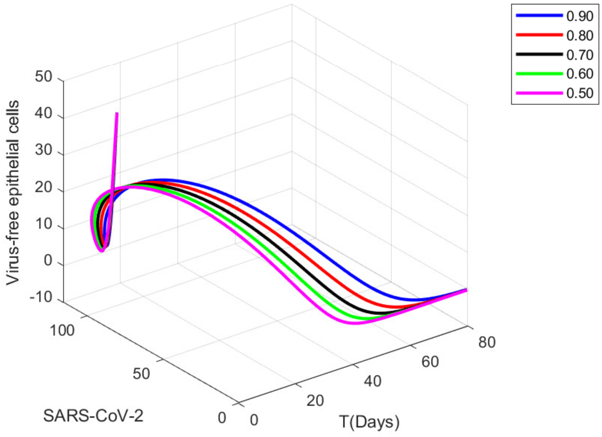
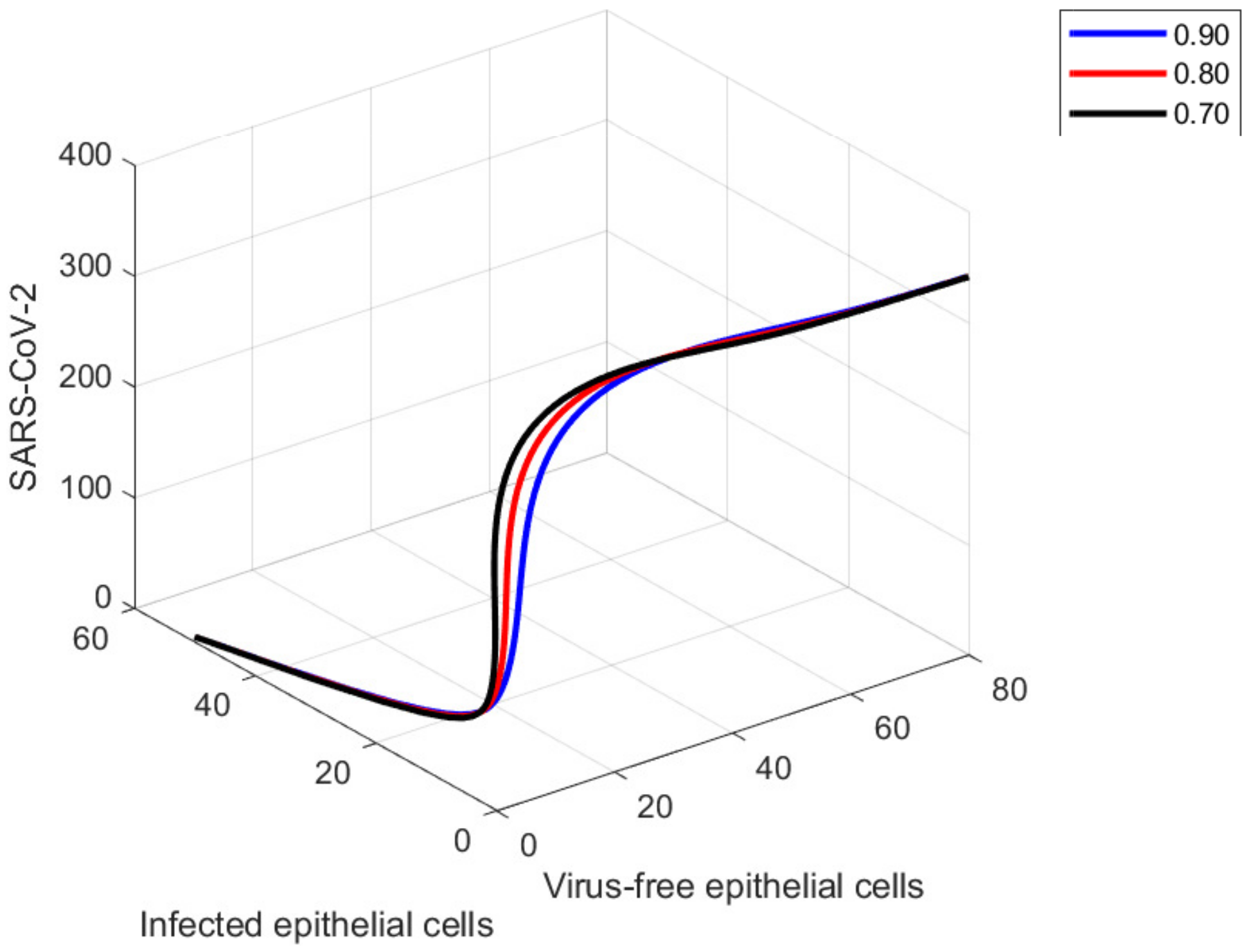
In this section, we discuss the obtain approximate solutions of (31) graphically using the values of the parameters shown in Table 1 with different α values.
We conduct graphical representation to represent the solution effects of our model with different fractional-order α . By using MATLAB software, we set up an algorithm to simulate the results in Figure 4, Figure 5, Figure 6, Figure 7, Figure 8 and Figure 9. For this, we consider some appropriate values used in the model for the parameters in Table 1. The parameter values of the model (3) have been estimated based on chest radiograph score data [5] using the Monte Carlo Markov Chain method. We utilize that parameter; more specifically, E p ( 0 ) = 50 , I p ( 0 ) = 50 , and F ( 0 ) = 100 .
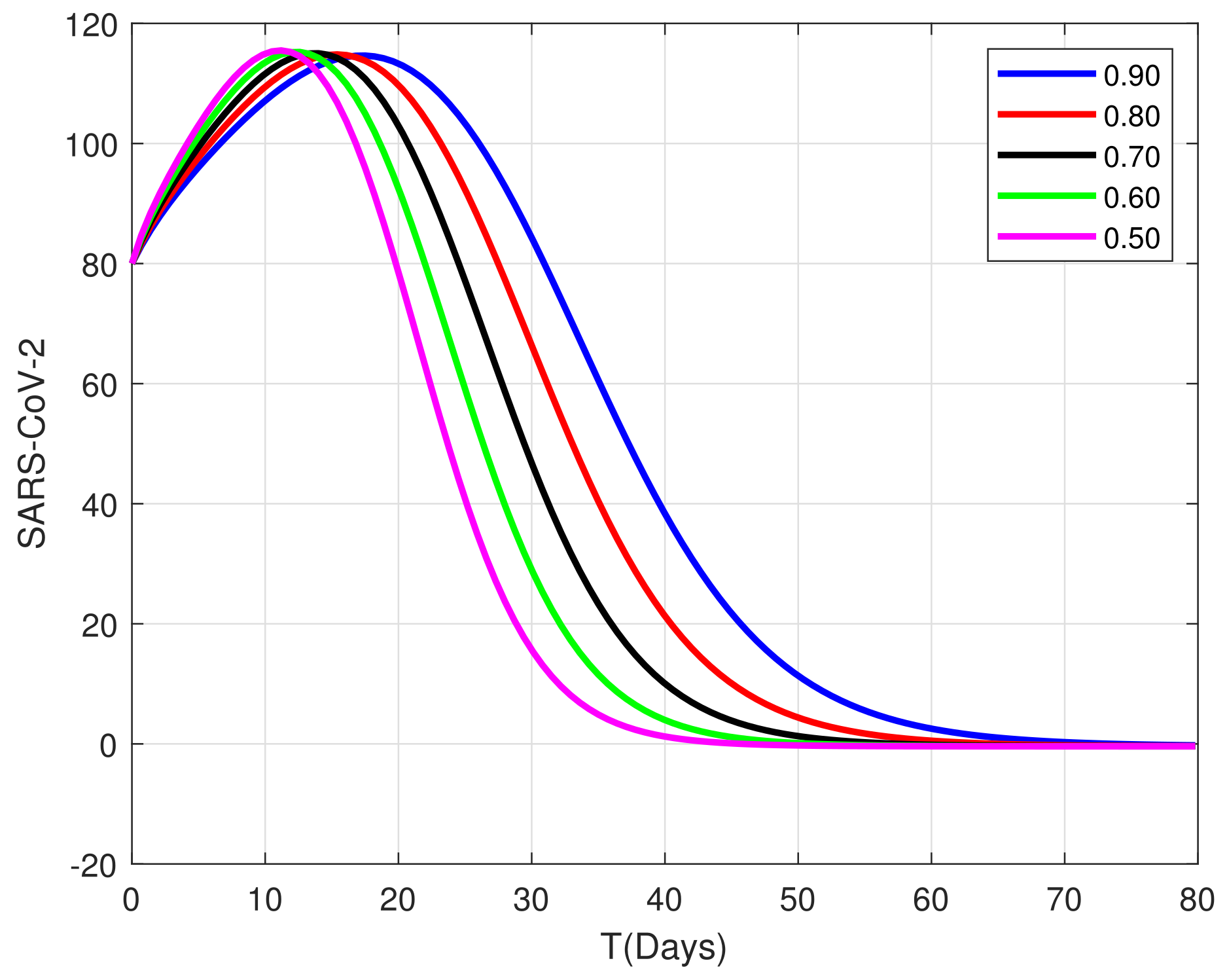
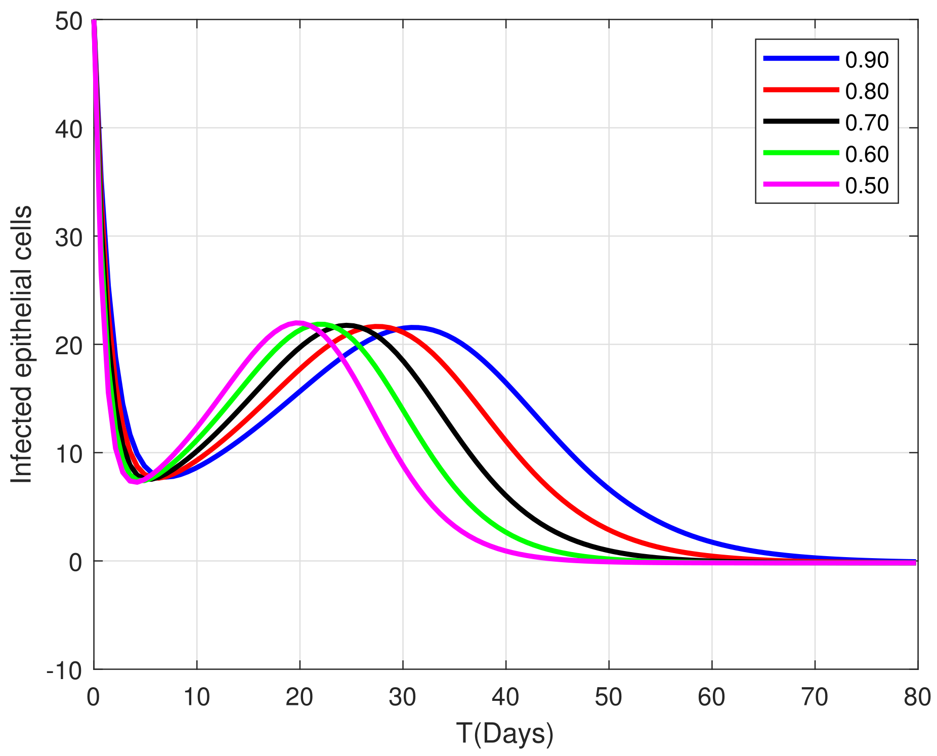
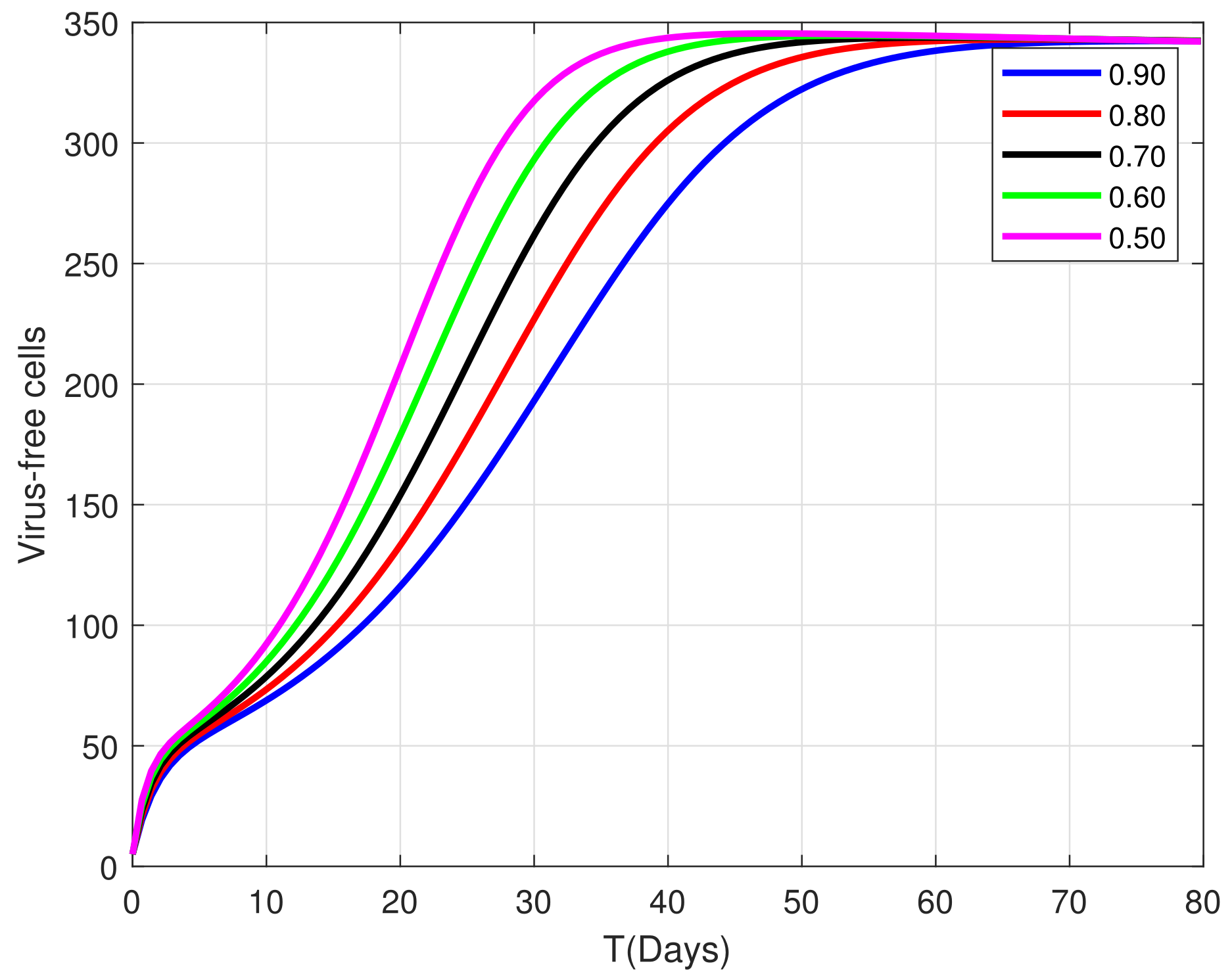
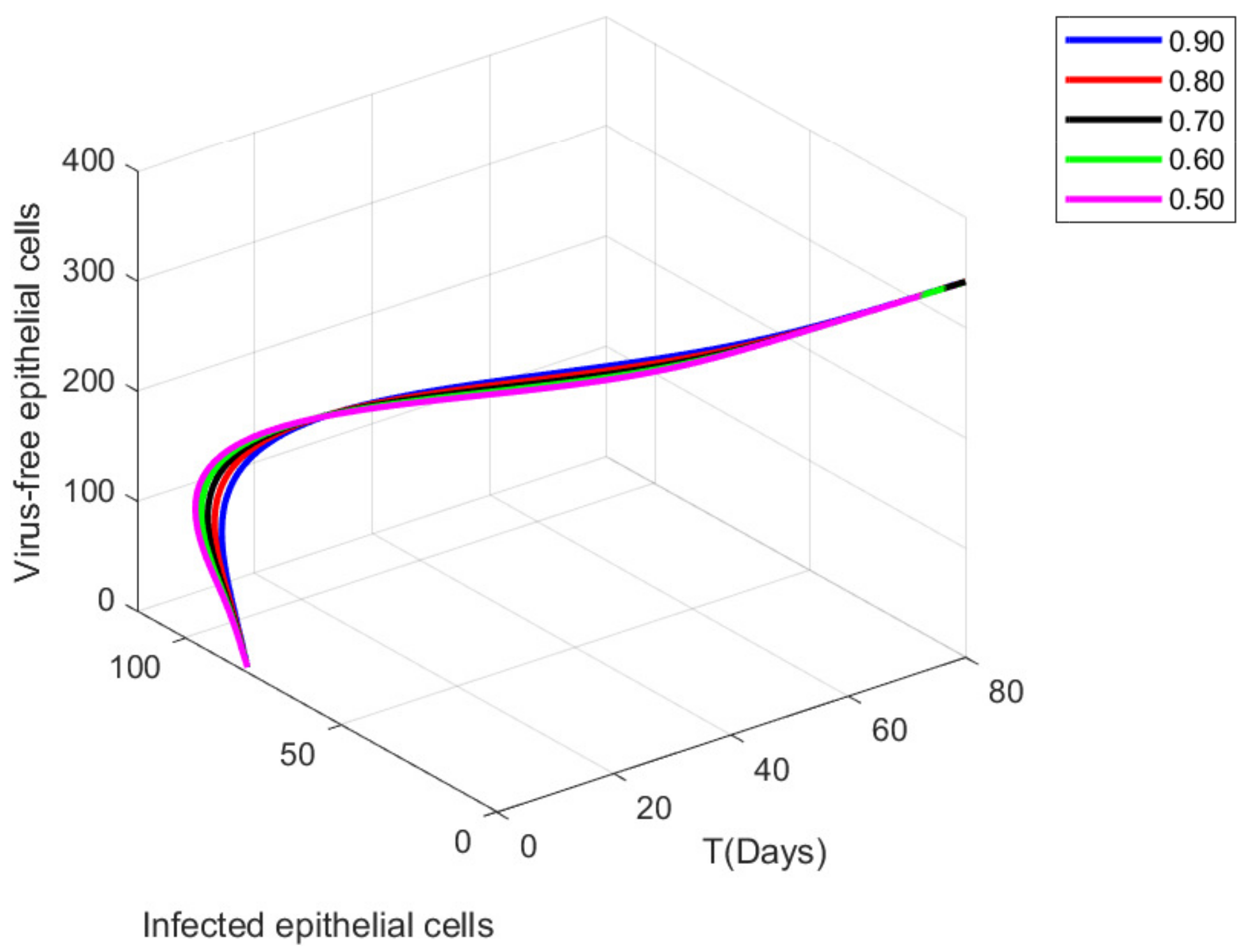
In Figure 4, we take the fractional-order α = 0.9 , which is close to the integer-order α = 1 . For this model, the results obtained from the fractional-order model of SARS-CoV-2 are very similar to those of the integer-order model [5]. Further, Figure 5, Figure 6, Figure 7, Figure 8 and Figure 9 show series plots of the approximate solutions (31) with the fractional orders slowly decreasing as follows: α = 0.90 , 0.80 , 0.70 , 0.60 , 0.50 . We observe from these graphs that the virus-infected, virus-free epithelial and the virus-free curves have approximately the same trend for different values of α . However, their convergence toward stability of the virus-infected epithelial is slightly changed. There is a notable difference in the graph at order 0.90 and 0.50. We also note that the equilibrium points are the same for the different fractional orders in Figure 4, Figure 5, Figure 6, Figure 7, Figure 8 and Figure 9, but the equilibrium points of the virus-infected epithelial go to the fixed point over a longer period when the fractional-order increases.
From the above plotting, we have concluded that the infection rate γ can be low. This is because, if we take the greater infection rate in such a way that R 0 > 1 , the infection prevails in the body since the virus cannot be controlled. However, if the infection rate γ is lower than R 0 < 1 , this leads to being controlled by the virus-infected epithelial cells rate in the body. Otherwise, the number of virus-free epithelial cells will decrease. Such infected virus epithelial cells and the virus-free cells will not stabilize very quickly in a body with time. In this case, the patient’s condition will vitiate with time. We also conclude that the fractional derivative is the generalization of the integer-order derivative. We use fractional-order to obtain good accuracy and reduce the possible errors arising from the mistreated parameters in the distributed modeling system and the system with memory.

10. Conclusions

This article presents a Caputo fractional-order model for the within-host dynamics of SARS-CoV-2. First, we found the existence and uniqueness of the model’s solution by using the fixed point theory. We obtained the disease-free and endemic equilibrium points. The critical parameter (reproduction number) R 0 was determined using the next-generation matrix approach. Moreover, we developed the considered model’s local and global stability conditions.
Further, we calculated the approximate solution to the model (3) via a powerful method due to Euler. Finally, graphical representations of the obtained approximate solutions were performed to verify the theoretical analysis using MATLAB. By biology, an infection will be cleaned from a human body when the basic reproduction number R 0 < 1 is approached; otherwise, therapy must be used to minimize and eliminate the infection from the body. Additionally, it was shown that an infection will continue for any level of viral load in the host’s body if the basic reproduction number is greater than one. For the eradication of the virus from an infected human body, our future work will include using various treatment strategies and control parameters in this model.

Author Contributions

Conceptualization, I.U.H.; methodology, I.U.H. and M.Y.; software, I.U.H.; validation, M.Y. and A.A.; investigation, I.U.H.; resources, A.A.; data curation, M.Y.; writing—original draft preparation, I.U.H. and N.A.; writing—review and editing, M.Y.; visualization, M.Y. and N.A.; supervision, N.A.; project administration, N.A. and A.A. All authors have read and agreed to the published version of the manuscript.

Funding

This research received no specific grant from any funding agency in the public, commercial, or not-for-profit sectors.

Acknowledgments

Authors are very much thankful for the anonymous reviewers and editors for their great efforts and comments that have improved the quality of the paper.

Conflicts of Interest

The authors declare that they have no conflict of interest.

References

  1. Reusken, C.B.; Buiting, A.; Bleeker-Rovers, C.; Diederen, B.; Hooiveld, M.; Friesema, I.; Koopmans, M.; Kortbeek, T.; Lutgens, S.P.; Meijer, A.; et al. Rapid assessment of regional SARS-CoV-2 community transmission through a convenience sample of healthcare workers, the Netherlands, March 2020. Eurosurveillance 2020, 25, 2000334. [Google Scholar] [CrossRef]
  2. Zhou, P.; Yang, X.L.; Wang, X.G.; Hu, B.; Zhang, L.; Zhang, W.; Si, H.R.; Zhu, Y.; Li, B.; Huang, C.L.; et al. Discovery of a novel coronavirus associated with the recent pneumonia outbreak in humans and its potential bat origin. BioRxiv 2020, 22, 914952. [Google Scholar]
  3. Miron, V.D. COVID-19 in the pediatric population and parental perceptions. Germs 2020, 10, 294. [Google Scholar] [CrossRef] [PubMed]
  4. Liang, K. Mathematical model of infection kinetics and its analysis for COVID-19, SARS and MERS. Infect. Genet. Evol. 2020, 82, 104306. [Google Scholar] [CrossRef] [PubMed]
  5. Li, C.; Xu, J.; Liu, J.; Zhou, Y. The within-host viral kinetics of SARS-CoV-2. bioRxiv 2020, 17, 234. [Google Scholar] [CrossRef]
  6. Mason, R.J. Pathogenesis of COVID-19 from a cell biology perspective. Eur. Respir. J. 2020, 55, 2000607. [Google Scholar] [CrossRef]
  7. World Health Orgnization. Naming the Coronavirus Disease (COVID-19) and the Virus That Causes It. 2020. Available online: https://www.who.int/emergencies/diseases/novel-coronavirus-2019/technical-guidance/naming-the-coronavirus-disease-(covid-2019)-and-the-virus-that-causes-it (accessed on 22 September 2022).
  8. Yang, C.; Wang, J. A mathematical model for the novel coronavirus epidemic in Wuhan, China. Math. Biosci. Eng. 2020, 17, 2853–2861. [Google Scholar] [CrossRef]
  9. Sinan, M.; Leng, J.; Anjum, M.; Fiaz, M. Asymptotic behavior and semi-analytic solution of a novel compartmental biological model. Math. Model. Numer. Simul. Appl. 2022, 2, 88–107. [Google Scholar] [CrossRef]
  10. Tang, B.; Bragazzi, N.L.; Li, Q.; Tang, S.; Xiao, Y.; Wu, J. An updated estimation of the risk of transmission of the novel coronavirus (2019-nCov). Infect. Dis. Model. 2020, 5, 248–255. [Google Scholar] [CrossRef]
  11. Kochańczyk, M.; Grabowski, F.; Lipniacki, T. Dynamics of COVID-19 pandemic at constant and time-dependent contact rates. Math. Model. Nat. Phenom. 2020, 15, 28. [Google Scholar] [CrossRef]
  12. Naik, P.A.; Yavuz, M.; Qureshi, S.; Zu, J.; Townley, S. Modeling and analysis of COVID-19 epidemics with treatment in fractional derivatives using real data from Pakistan. Eur. Phys. J. Plus 2020, 135, 1–42. [Google Scholar] [CrossRef]
  13. Allegretti, S.; Bulai, I.M.; Marino, R.; Menandro, M.A.; Parisi, K. Vaccination effect conjoint to fraction of avoided contacts for a Sars-Cov-2 mathematical model. Math. Model. Numer. Simul. Appl. 2021, 1, 56–66. [Google Scholar] [CrossRef]
  14. Özköse, F.; Yavuz, M.; Şenel, M.T.; Habbireeh, R. Fractional order modelling of omicron SARS-CoV-2 variant containing heart attack effect using real data from the United Kingdom. Chaos Solitons Fractals 2022, 157, 111954. [Google Scholar] [CrossRef]
  15. Haq, I.U.; Ali, N.; Nisar, K.S. An optimal control strategy and Grünwald-Letnikov finite-difference numerical scheme for the fractional-order COVID-19 model. Math. Model. Numer. Simul. Appl. 2022, 2, 108–116. [Google Scholar] [CrossRef]
  16. Özköse, F.; Yavuz, M. Investigation of interactions between COVID-19 and diabetes with hereditary traits using real data: A case study in Turkey. Comput. Biol. Med. 2022, 141, 105044. [Google Scholar] [CrossRef]
  17. Ikram, R.; Khan, A.; Zahri, M.; Saeed, A.; Yavuz, M.; Kumam, P. Extinction and stationary distribution of a stochastic COVID-19 epidemic model with time-delay. Comput. Biol. Med. 2022, 141, 105115. [Google Scholar] [CrossRef]
  18. Naik, P.A.; Eskandari, Z.; Yavuz, M.; Zu, J. Complex dynamics of a discrete-time Bazykin–Berezovskaya prey-predator model with a strong Allee effect. J. Comput. Appl. Math. 2022, 413, 114401. [Google Scholar] [CrossRef]
  19. Moussouni, N.; Aliane, M. Optimal control of COVID-19. Int. J. Optim. Control Theor. Appl. 2021, 11, 114–122. [Google Scholar] [CrossRef]
  20. Hamou, A.A.; Rasul, R.R.; Hammouch, Z.; Özdemir, N. Analysis and dynamics of a mathematical model to predict unreported cases of COVID-19 epidemic in Morocco. Comput. Appl. Math. 2022, 41, 1–33. [Google Scholar] [CrossRef]
  21. Evirgen, F. Transmission of Nipah virus dynamics under Caputo fractional derivative. J. Comput. Appl. Math. 2023, 418, 114654. [Google Scholar] [CrossRef]
  22. Du, S.Q.; Yuan, W. Mathematical modeling of interaction between innate and adaptive immune responses in COVID-19 and implications for viral pathogenesis. J. Med. Virol. 2020, 92, 1615–1628. [Google Scholar] [CrossRef]
  23. Abuin, P.; Anderson, A.; Ferramosca, A.; Hernandez-Vargas, E.A.; Gonzalez, A.H. Characterization of SARS-CoV-2 dynamics in the host. Annu. Rev. Control 2020, 50, 457–468. [Google Scholar] [CrossRef]
  24. Nath, B.J.; Dehingia, K.; Mishra, V.N.; Chu, Y.M.; Sarmah, H.K. Mathematical analysis of a within-host model of SARS-CoV-2. Adv. Differ. Equ. 2021, 2021, 1–11. [Google Scholar] [CrossRef]
  25. Agarwal, P.; Deniz, S.; Jain, S.; Alderremy, A.A.; Aly, S. A new analysis of a partial differential equation arising in biology and population genetics via semi analytical techniques. Phys. A Stat. Mech. Appl. 2020, 542, 122769. [Google Scholar] [CrossRef]
  26. Lei, S.; Jiang, F.; Su, W.; Chen, C.; Chen, J.; Mei, W.; Zhan, L.Y.; Jia, Y.; Zhang, L.; Liu, D.; et al. Clinical characteristics and outcomes of patients undergoing surgeries during the incubation period of COVID-19 infection. EClinicalMedicine 2020, 21, 100331. [Google Scholar] [CrossRef]
  27. Wu, J.T.; Leung, K.; Leung, G.M. Nowcasting and forecasting the potential domestic and international spread of the 2019-nCoV outbreak originating in Wuhan, China: A modelling study. Lancet 2020, 395, 689–697. [Google Scholar] [CrossRef]
  28. Chan, J.F.W.; Yuan, S.; Kok, K.H.; To, K.K.W.; Chu, H.; Yang, J.; Xing, F.; Liu, J.; Yip, C.C.Y.; Poon, R.W.S.; et al. A familial cluster of pneumonia associated with the 2019 novel coronavirus indicating person-to-person transmission: A study of a family cluster. Lancet 2020, 395, 514–523. [Google Scholar] [CrossRef]
  29. Letko, M.; Munster, V. Functional assessment of cell entry and receptor usage for lineage B β-coronaviruses, including 2019-nCoV. bioRxiv 2020. [Google Scholar] [CrossRef]
  30. Liu, J.; Liao, X.; Qian, S.; Yuan, J.; Wang, F.; Liu, Y.; Wang, Z.; Wang, F.S.; Liu, L.; Zhang, Z. Community transmission of severe acute respiratory syndrome coronavirus 2, Shenzhen, China, 2020. Emerg. Infect. Dis. 2020, 26, 1320. [Google Scholar] [CrossRef]
  31. Agarwal, P.; Nieto, J.J.; Ruzhansky, M.; Torres, D.F. Analysis of Infectious Disease Problems (Covid-19) and Their Global Impact; Springer: Berlin/Heidelberg, Germany, 2021. [Google Scholar]
  32. Yavuz, M.; Coşar, F.Ö.; Günay, F.; Özdemir, F.N. A new mathematical modeling of the COVID-19 pandemic including the vaccination campaign. J Model. Simul. 2021, 9, 299–321. [Google Scholar] [CrossRef]
  33. Tuite, A.R.; Fisman, D.N.; Greer, A.L. Mathematical modelling of COVID-19 transmission and mitigation strategies in the population of Ontario, Canada. CMAJ 2020, 192, E497–E505. [Google Scholar] [CrossRef] [PubMed] [Green Version]
  34. Marovich, M.; Mascola, J.R.; Cohen, M.S. Monoclonal antibodies for prevention and treatment of COVID-19. JAMA 2020, 324, 131–132. [Google Scholar] [CrossRef] [PubMed]
  35. Li, G.; Fan, Y.; Lai, Y.; Han, T.; Li, Z.; Zhou, P.; Pan, P.; Wang, W.; Hu, D.; Liu, X.; et al. Coronavirus infections and immune responses. J. Med. Virol. 2020, 92, 424–432. [Google Scholar] [CrossRef] [PubMed]
  36. Harapan, H.; Itoh, N.; Yufika, A.; Winardi, W.; Keam, S.; Te, H.; Megawati, D.; Hayati, Z.; Wagner, A.L.; Mudatsir, M. Coronavirus disease 2019 (COVID-19): A literature review. J. Infect. Public Health 2020, 13, 667–673. [Google Scholar] [CrossRef]
  37. Chen, T.M.; Rui, J.; Wang, Q.P.; Zhao, Z.Y.; Cui, J.A.; Yin, L. A mathematical model for simulating the phase-based transmissibility of a novel coronavirus. Infect. Dis. Poverty 2020, 9, 1–8. [Google Scholar] [CrossRef]
  38. Ahmed, I.; Baba, I.A.; Yusuf, A.; Kumam, P.; Kumam, W. Analysis of Caputo fractional-order model for COVID-19 with lockdown. Adv. Differ. Equ. 2020, 2020, 1–14. [Google Scholar] [CrossRef]
  39. Baba, I.A.; Nasidi, B.A. Fractional order model for the role of mild cases in the transmission of COVID-19. Chaos Solitons Fractals 2021, 142, 110374. [Google Scholar] [CrossRef]
  40. Hamdan, N.; Kilicman, A. Analysis of the fractional order dengue transmission model: A case study in Malaysia. Adv. Differ. Equ. 2019, 2019, 1–13. [Google Scholar] [CrossRef]
  41. Khan, M.; Khan, A.; Elsonbaty, A.; Elsadany, A. Modeling and simulation results of a fractional dengue model. Eur. Phys. J. Plus 2019, 134, 379. [Google Scholar] [CrossRef]
  42. Hammouch, Z.; Yavuz, M.; Özdemir, N. Numerical solutions and synchronization of a variable-order fractional chaotic system. Math. Model. Numer. Simul. Appl. 2021, 1, 11–23. [Google Scholar] [CrossRef]
  43. Din, A.; Abidin, M.Z. Analysis of fractional-order vaccinated Hepatitis-B epidemic model with Mittag-Leffler kernels. Math. Model. Numer. Simul. Appl. 2022, 2, 59–72. [Google Scholar] [CrossRef]
  44. Kalidass, M.; Zeng, S.; Yavuz, M. Stability of Fractional-Order Quasi-Linear Impulsive Integro-Differential Systems with Multiple Delays. Axioms 2022, 11, 308. [Google Scholar] [CrossRef]
  45. Caputo, M.; Fabrizio, M. A new definition of fractional derivative without singular kernel. Prog. Fract. Differ. Appl. 2015, 1, 73–85. [Google Scholar]
  46. Atangana, A.; Baleanu, D. New fractional derivatives with nonlocal and non-singular kernel: Theory and application to heat transfer model. arXiv 2016, arXiv:1602.03408. [Google Scholar] [CrossRef]
  47. Lee, H.Y.; Topham, D.J.; Park, S.Y.; Hollenbaugh, J.; Treanor, J.; Mosmann, T.R.; Jin, X.; Ward, B.M.; Miao, H.; Holden-Wiltse, J.; et al. Simulation and prediction of the adaptive immune response to influenza A virus infection. J. Virol. 2009, 83, 7151–7165. [Google Scholar] [CrossRef]
  48. Higazy, M. Novel fractional order SIDARTHE mathematical model of COVID-19 pandemic. Chaos Solitons Fractals 2020, 138, 110007. [Google Scholar] [CrossRef]
  49. Ahmad, S.; Ullah, A.; Al-Mdallal, Q.M.; Khan, H.; Shah, K.; Khan, A. Fractional Order Mathematical Modeling of COVID-19 Transmission; Elsevier: Amsterdam, The Netherlands, 2020; Volume 139, p. 110256. [Google Scholar]
  50. Joshi, H.; Jha, B.K. Chaos of calcium diffusion in Parkinson’s infectious disease model and treatment mechanism via Hilfer fractional derivative. Math. Model. Numer. Simul. Appl. 2021, 1, 84–94. [Google Scholar]
  51. Yavuz, M.; Sene, N.; Yıldız, M. Analysis of the influences of parameters in the fractional second-grade fluid dynamics. Mathematics 2022, 10, 1125. [Google Scholar] [CrossRef]
  52. Kilbas, A.; Trujillo, J. Differential equations of fractional order: Methods, results and problems. II. Appl. Anal. 2002, 81, 435–493. [Google Scholar] [CrossRef]
  53. Diekmann, O.; Heesterbeek, J.; Roberts, M.G. The construction of next-generation matrices for compartmental epidemic models. J. R. Soc. Interface 2010, 7, 873–885. [Google Scholar] [CrossRef]
  54. Ahmed, E.; Elgazzar, A. On fractional order differential equations model for nonlocal epidemics. Phys. A Stat. Mech. Its Appl. 2007, 379, 607–614. [Google Scholar] [CrossRef]
  55. Ahmady, N.; Allahviranloo, T.; Ahmady, E. A modified Euler method for solving fuzzy differential equations under generalized differentiability. Comput. Appl. Math. 2020, 39, 1–21. [Google Scholar] [CrossRef]
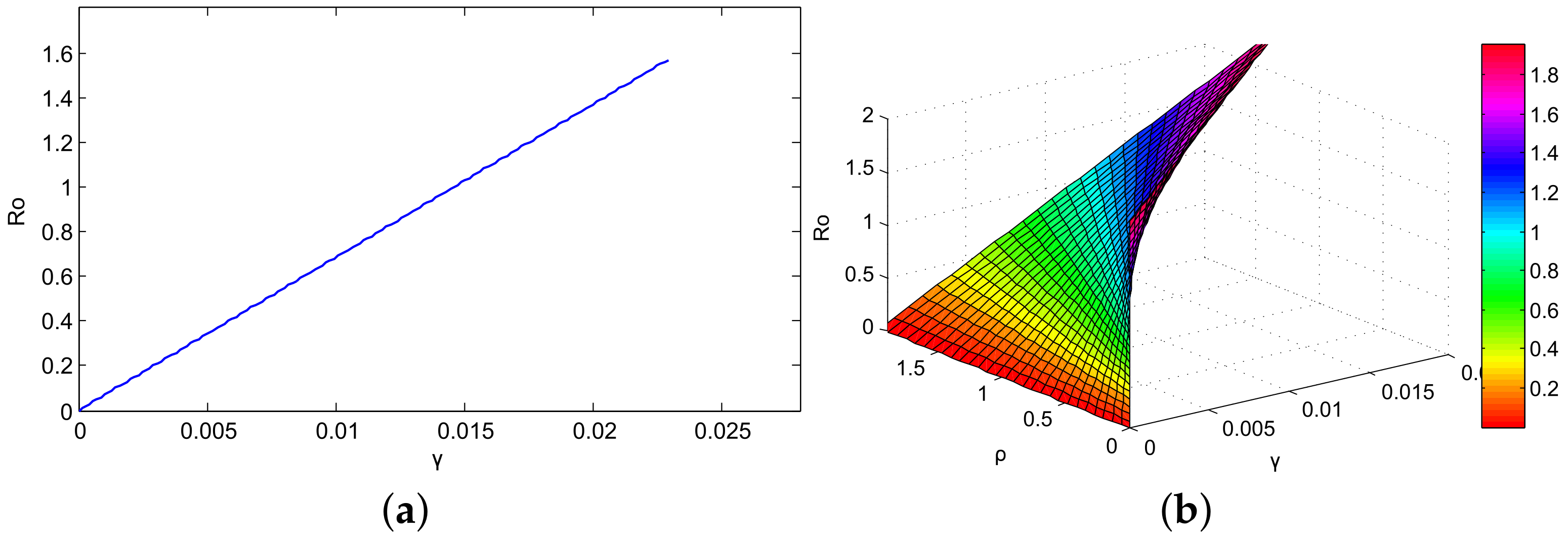
Figure 1. It is clear that, when R 0 < 1 , the model (3) has no endemic equilibrium and the disease-free equilibrium is stable. (a) Variation of R 0 with respect to the transmission rate γ . (b) Impact of γ and ρ on R 0 .
Mca 27 00082 g001
Figure 2. Simulation of the numbers of E p , I p , and F when R 0 < 1 with (a) three-dimensional plot and (b) two-dimensional plot.
Mca 27 00082 g002
Figure 3. Dynamics of the numbers of virus-infected epithelial cells, SARS-CoV-2 virus and virus-free epithelial cells when R 0 > 1 with (a) three-dimensional plot and (b) two-dimensional plot.
Mca 27 00082 g003
Figure 4. Graphical representation of the approximate solutions of the SARS-CoV-2 model for order α = 0.9 , 0.8 , 0.7 , 0.6 , 0.5 .
Mca 27 00082 g004
Figure 5. Graphical representation of the approximate solutions of the infected virus epithelial cells for fractional order α = 0.9 , 0.8 , 0.7 , 0.6 , 0.5 .
Mca 27 00082 g005
Figure 6. Graphical representation of the approximate solutions of the virus-free epithelial cells for fractional order α = 0.9 , 0.8 , 0.7 , 0.6 , 0.5 .
Mca 27 00082 g006
Figure 7. Graphical representation of the virus-infected epithelial cells and virus-free epithelial cells for fractional order α = 0.9 , 0.8 , 0.7 , 0.6 , 0.5 when R 0 < 1 .
Mca 27 00082 g007
Figure 8. Graphical representation of the SARS-CoV-2 and virus-free epithelial cells for fractional order α = 0.9 , 0.8 , 0.7 , 0.6 , 0.5 when R 0 < 1 .
Mca 27 00082 g008
Figure 9. Graphical representation of the SARS-CoV-2, virus-infected epithelial cells, and virus-free epithelial cells of approximate solutions for fractional order α = 0.9 , 0.8 , 0.7 .
Mca 27 00082 g009
Table 1. Parameters and their values.
SymbolParameter ValuesReferences
δ 0.09932Assumed
β 0.229Assumed
ω 0.0326Assumed
γ 0.001[5]
ρ 0.7492[5]
E p ( 0 ) 80Assumed
I ( 0 ) 50Assumed
F ( 0 ) 5Assumed
Publisher’s Note: MDPI stays neutral with regard to jurisdictional claims in published maps and institutional affiliations.