Treatment Effect Performance of the X-Learner in the Presence of Confounding and Non-Linearity
Abstract
:1. Introduction
- The above-mentioned studies [1,4,12], were carried out on real-life data where the true treatment effects were not known. Studies are therefore required where the true treatment effect is known, in order to evaluate the accuracy of the X-Learner method. Smith et al. [1] attempted to validate the X-Learner method by comparing it with PSM estimations; however the ground truth average treatment effect (ATE) was still not known. Beemer et al. [4] and Beemer et al. [12] applied this method to student performance data but did not attempt to validate with alternative methods.
- Kunzel et al. [11] did carry out simulation studies with known treatment effects; however they did not compare these results with traditional regression methods for estimating treatment effects. This is important because as we will see, the X-Learner method is a multi-step complicated computation, and if it does not provide clear benefits over traditional methods, then it might not be worthwhile.
Main Contributions
2. Related Work
3. Observational Studies and Treatment Effects
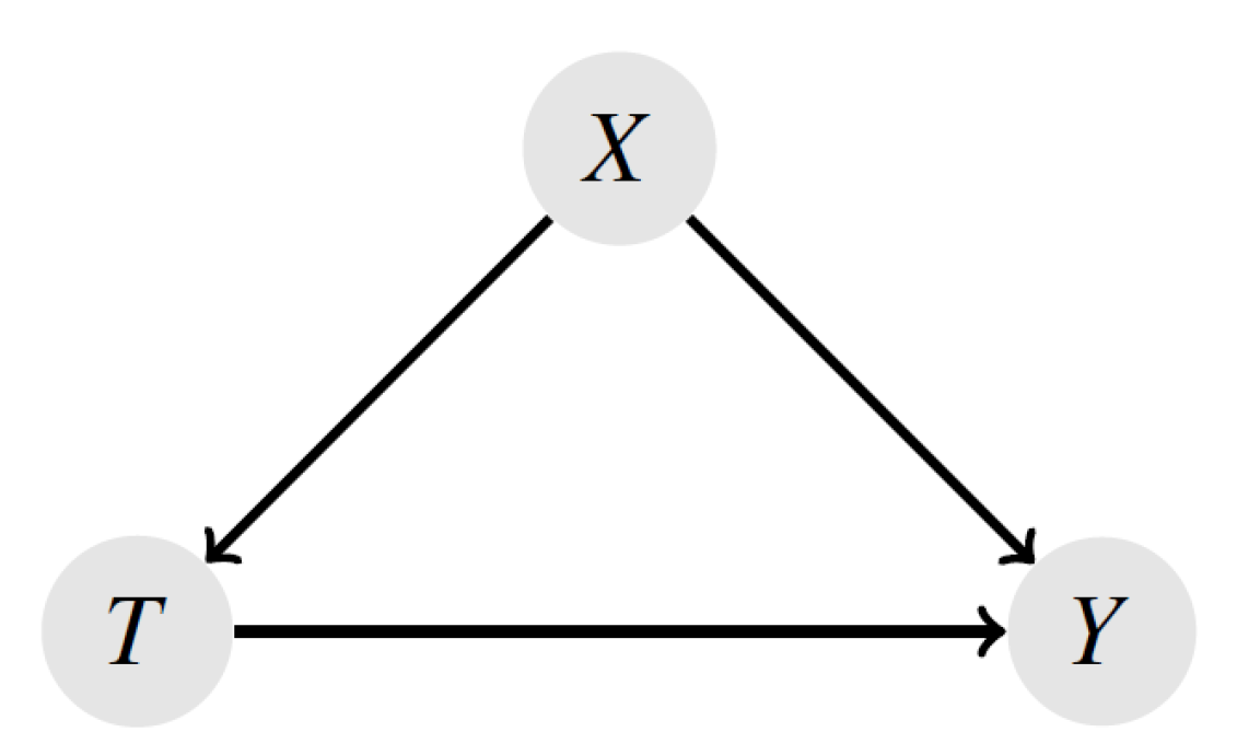
4. Confounding Bias in Observational Studies
The Counterfactual
5. X-Learner Method
- Split the entire dataset into treated and control groups.
- Train a machine learning model on the treated group and a model on the control group.
- Predict treated group counterfactual, , by feeding the treated group input features, , into the control group model . Predict control group counterfactual, , by feeding the control group input features, , into the treatment model .
- Estimate the true treatment effect using Equation (2).
6. Simulations
6.1. Dataset Features
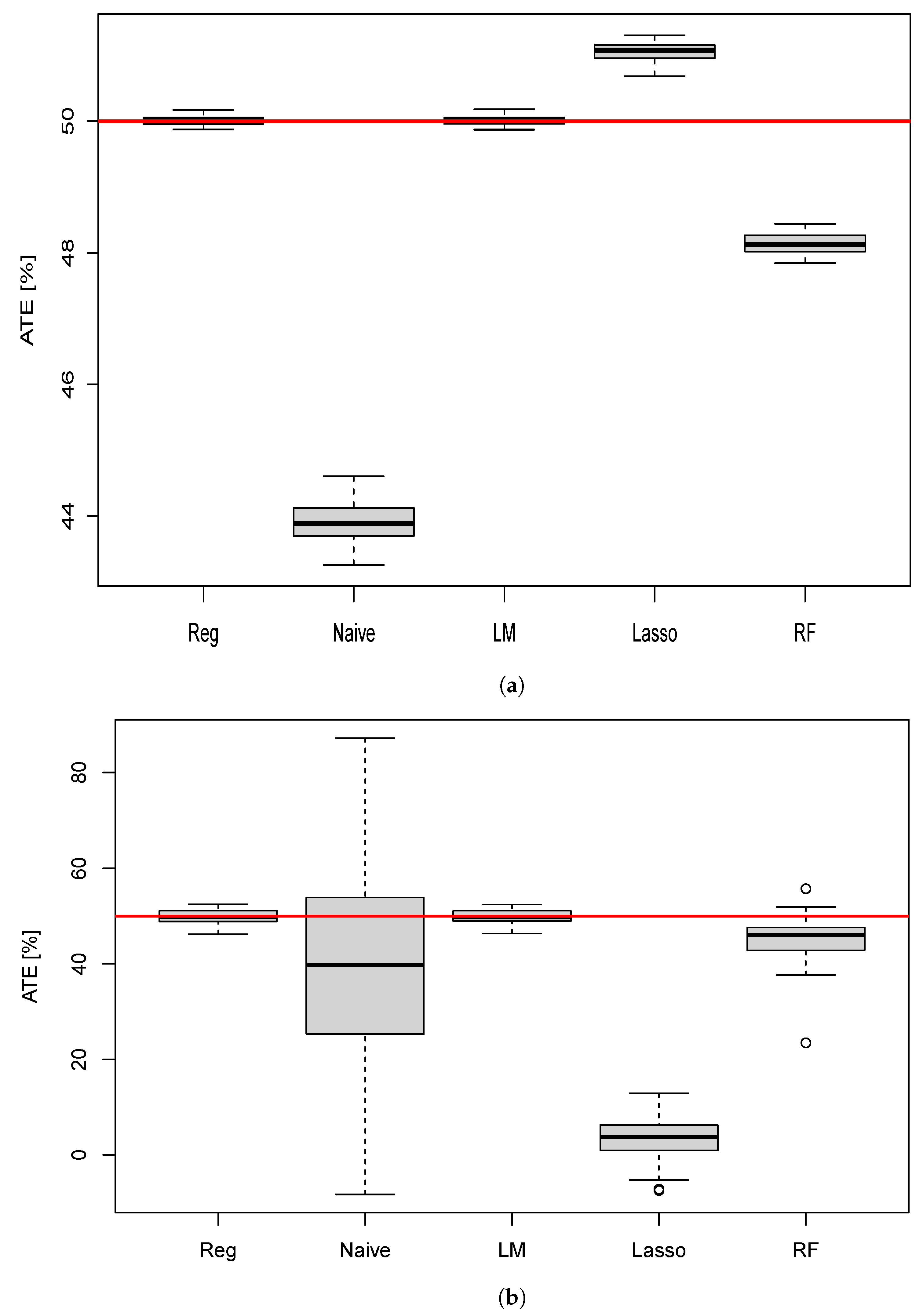
- Simulation A: Confounding; linear dataset.
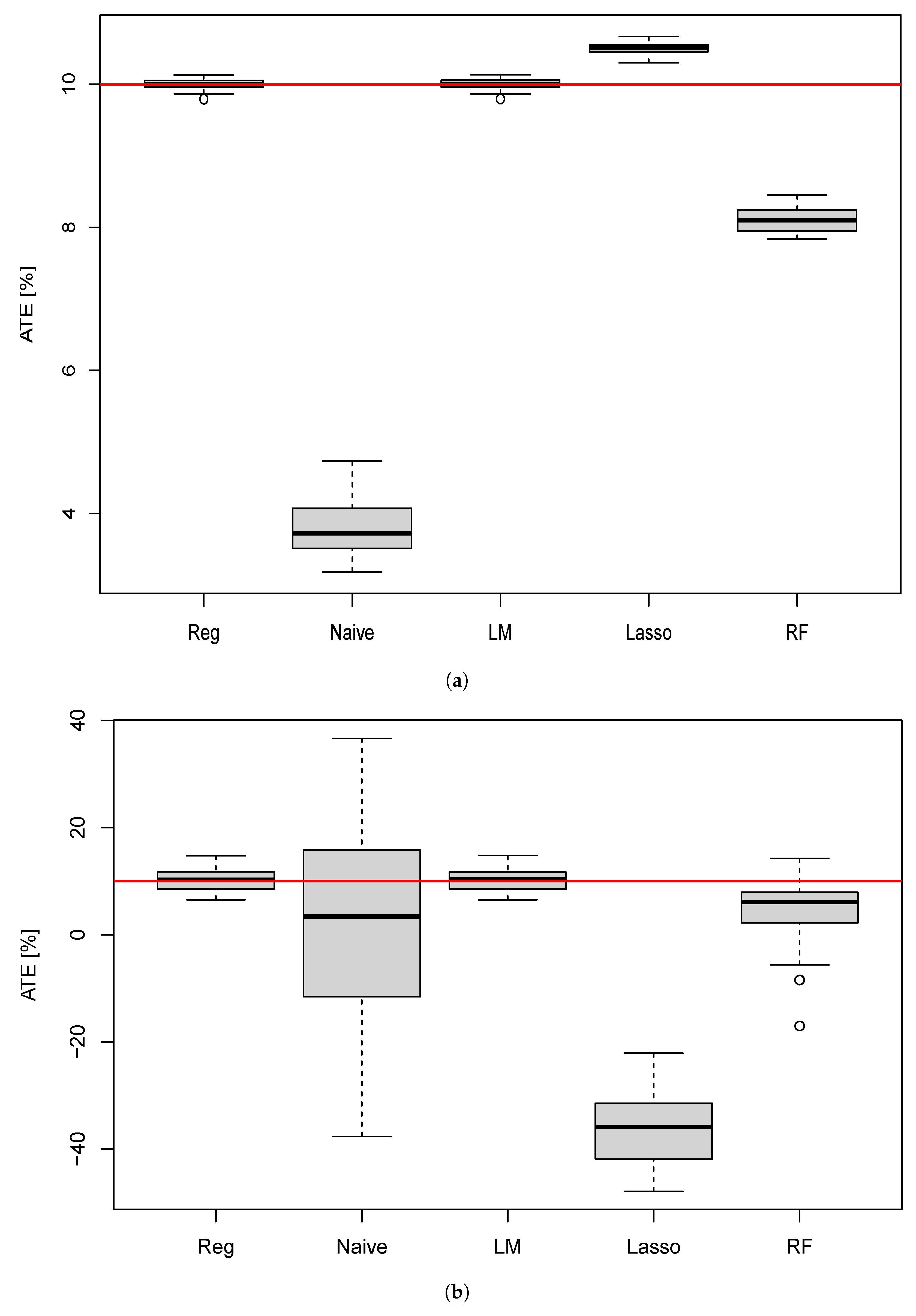
- Simulation B: Confounding, non-linear (squared) dataset.
6.1.1. Simulation A: Linear and Confounding
6.1.2. Simulation B: Non-Linear (Squared) and Confounding
6.1.3. Range of Values
6.1.4. Pseudocode for Simulating the X-Learner Method
| Pseudocode 1 for each run of a simulation of the X-Learner method |
| 1. Generate data: to , T and Y as per Table 1 and Equations (3) and (5) depending on type of simulation. |
| 2. Split dataset into treated and control groups. |
| 3. Train the three models (linear model , lasso , random forest ) on treated group; train the three models (linear model , lasso , random forest ) on control group. |
| 4. Feed treated group input features to into linear model , lasso , random forest to predict treated group counterfactual for each model; feed control group to into , and to predict control group counterfactual for each model. |
| 5. Compute for the three models, as per Equation (2) and store. |
7. Linear Regression, Lasso and Random Forest Models
8. Baseline Methods
9. Software
10. Results
10.1. ATE Estimation for the Different Methods
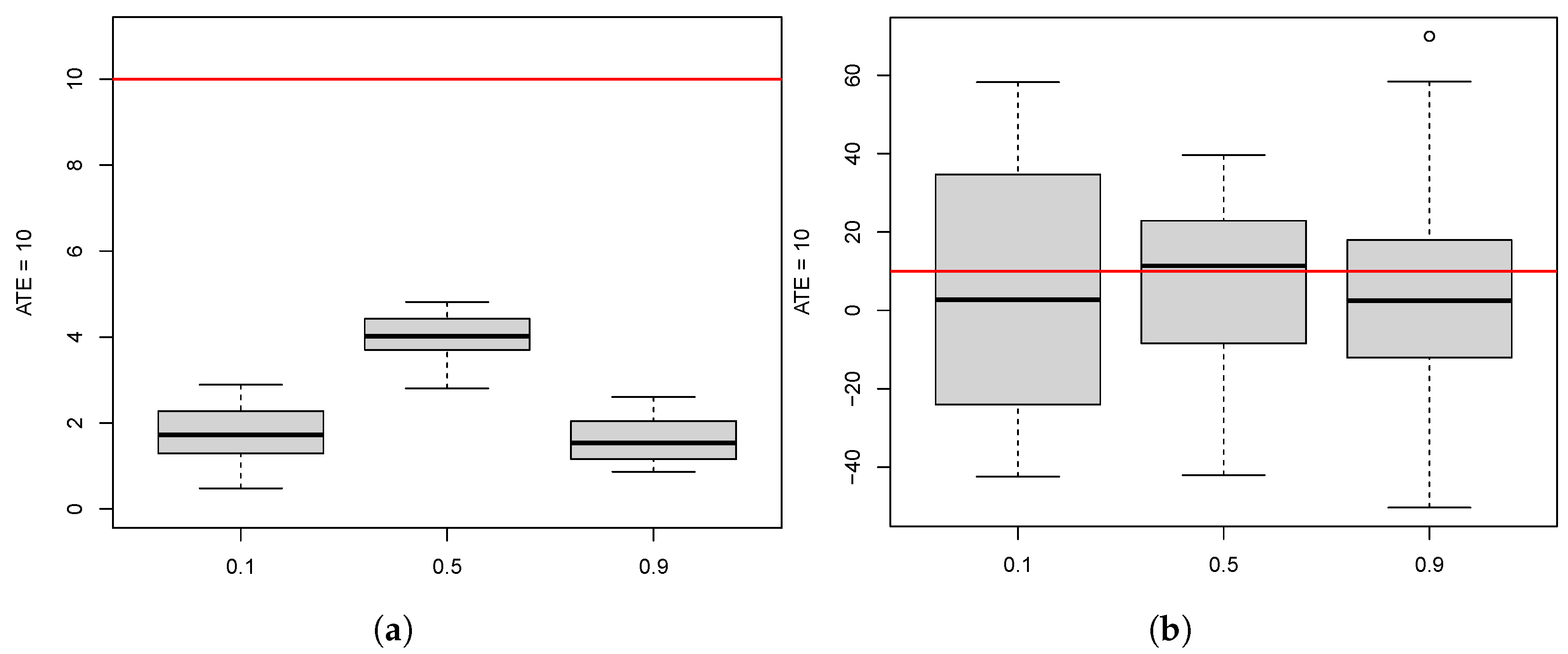
10.2. Effect of Participation Rate
11. Discussion
Limitations and Recommendations for Future Work
- The confounding simulation was based on a single observable confounding feature affecting both the treatment and output. We did not look at multiple confounding features. We anticipate that more confounding would introduce larger errors. Future work can look at more observable confounders.
- We assumed that the treatment effect was constant. This implies that all treated people experienced the same effect of the treatment, which is real life is unfeasible. Future work would introduce non-constant treatment effects into the data.
- We did not simulate hidden confounding which is common in observational studies. The assumption in this study was no hidden confounding. Future work could study the results of simulations that include hidden confounding by generating datasets that include the confounding variable but then exclude it when carrying out methods such as the X-Learner method.
- More research is needed to understand how different models, such as neural networks or boosting will perform. More thorough tuning of model hyperparameters is suggested for more complex models, such as neural networks, random forest, and boosting models.
- When estimating treatment effects using model predictions, we used the same model on both treated and control groups. For example, we used linear regression, or random forest, on both groups and estimated treatment effects. Future work could look at mixing up the models. For example, using a lasso model on a treated group and a random forest on the control and then estimating treatment effects.
- In a more general sense, it is hoped that future work would incorporate causal inference into AutoML. AutoML refers to automating the training of machine learning models [44,45]. Currently, no literature was found that incorporates causal inference into AutoML applications and this serves as a promising future application. Microsoft has developed causal inference applications that promise to perform end-to-end causal inference from raw data.
12. Statements and Declarations
Author Contributions
Funding
Data Availability Statement
Conflicts of Interest
Abbreviations
| ATE | Average treatment effect |
| RF | Random forest |
| LM | Linear regression model |
| PSM | Propensity score matching |
| IPTW | Inverse probability of treatment weighting |
| BART | Bayesian additive regression trees |
| RCT | Randomized controlled trials |
| DAG | Directed acyclic graph |
| SCM | Structural causal model |
References
- Smith, B.I.; Chimedza, C.; Bührmann, J.H. Global and individual treatment effects using machine learning methods. Int. J. Artif. Intell. Educ. 2020, 30, 431–458. [Google Scholar] [CrossRef]
- Smith, B.; Chimedza, C.; Bührmann, J.H. Measuring treatment effects of online videos on academic performance using difference-in-difference estimations. S. Afr. J. Ind. Eng. 2018, 32, 111–121. [Google Scholar] [CrossRef]
- Sneyers, E.; Witte, K.D. Interventions in higher education and their effect on student success: A meta-analysis. Educ. Rev. 2018, 70, 208–228. [Google Scholar] [CrossRef]
- Beemer, J.; Spoon, K.; He, L.; Fan, J.; Levine, R.A. Ensemble learning for estimating individualized treatment effects in student success studies. Int. J. Artif. Intell. Educ. 2017, 28, 315–335. [Google Scholar] [CrossRef]
- Williams, A.; Birch, E.; Hancock, P. The impact of online lecture recording on student performance. Australas. J. Educ. Technol. 2012, 28, 1–9. [Google Scholar] [CrossRef]
- Rosenbaum, P.R.; Rosenbaum, P. Briskman. Design of Observational Studies; Springer: New York, NY, USA, 2010; Volume 10. [Google Scholar]
- Rosenbaum, P.R. Design sensitivity in observational studies. Biometrika 2004, 91, 153–164. [Google Scholar] [CrossRef]
- Austin, P.C. An introduction to propensity score methods for reducing the effects of confounding in observational studies. Multivar. Behav. Res. 2011, 46, 399–424. [Google Scholar] [CrossRef] [Green Version]
- Ye, Y.; Kaskutas, L.A. Using propensity scores to adjust for selection bias when assessing the effectiveness of alchoholics anonymous in observational studies. Drug Alcohol Depend. 2009, 104, 56–64. [Google Scholar] [CrossRef] [Green Version]
- Stuart, E.A. Matching methods for causal inference: A review and a look forward. Stat. Sci. 2010, 25, 1–21. [Google Scholar] [CrossRef] [Green Version]
- Künzel, S.R.; Sekhon, J.S.; Bickerl, P.J.; Yu, B. Metalearners for estimating heterogeneous treatment effects using machine learning. Proc. Natl. Acad. Sci. USA 2019, 116, 4156–4165. [Google Scholar] [CrossRef] [Green Version]
- Beemer, J.; Spoon, K.; Fan, J.; Stronach, J.; Frazee, J.P.; Bohonak, A.J.; Levine, R.A. Assessing instructional modalities: Individualized treatment effects for personalized learning. J. Stat. Educ. 2018, 26, 31–39. [Google Scholar] [CrossRef] [Green Version]
- Neal, B. Introduction to causal inference: From a machine learning perspective. Course Lect. Notes 2020. [Google Scholar]
- Wieling, M.; Hofman, W. The impact of online video lecture recordings and automated feedback on student performance. Comput. Educ. 2010, 54, 992–998. [Google Scholar] [CrossRef]
- Bonnini, S.; Cavallo, G. A study on the satisfaction with distance learning of university students with disabilities: Bivariate regression analysis using a multiple permutation test. Stat. Appl. Ital. J. Appl. Stat. 2021, 33, 143–162. [Google Scholar]
- Graham, S.E.; Kurlaender, M. Using propensity scores in educational research. J. Educ. Res. 2010, 104, 340–353. [Google Scholar] [CrossRef]
- Kotsiantis, S.; Pierrakeas, C.; Pintelas, P. Predicting Students’ Performance in Distance Learning Using Machine Learning Techniques. Appl. Artif. Intell. 2004, 18, 411–426. [Google Scholar] [CrossRef]
- Kotsiantis, S.; Kanellopoulos, D.; Pintelas, P. Data preprocessing for supervised learning. Int. J. Comput. Sci. 2006, 1, 111–117. [Google Scholar]
- Nisa, M.; Mahmood, D.; Ahmed, G.; Khan, S.; Mohammed, M.; Damaševičius, R. Optimizing Prediction of YouTube Video Popularity Using XGBoost. Electronics 2021, 10, 2962. [Google Scholar]
- Natan, S.; Lazebnik, T.; Lerner, E. A distinction of three online learning pedagogic paradigms. SN Soc. Sci. 2022, 2, 46. [Google Scholar] [CrossRef]
- Korkmaz, C.; Correia, A.P. A review of research on machine learning in educational technology. Educ. Media Int. 2019, 56, 250–267. [Google Scholar] [CrossRef]
- Hassanpour, N.; Greiner, R. Learning disentangled representations for counterfactual regression. In Proceedings of the International Conference on Learning Representations, Addis Ababa, Ethiopia, 26–30 April 2020. [Google Scholar]
- Verma, S.; Boonsanong, V.; Hoang, M.; Hines, K.E.; Dickerson, J.P.; Shah, C. Counterfactual Explanations and Algorithmic Recourses for Machine Learning: A Review. arXiv 2020, arXiv:2010.10596. [Google Scholar]
- Athey, S. Machine learning and causal inference for policy evaluation. In Proceedings of the KDD’15 Proceedings of the 21th ACM SIGKDD International Conference on Knowledge Discovery and Data Mining, Sydney, Australia, 10–13 August 2015; pp. 5–6. [Google Scholar]
- Hill, J.L. Bayesian Nonparametric Modeling for Causal Inference. J. Comput. Graph. Stat. 2011, 20, 217–240. [Google Scholar] [CrossRef]
- Athey, S.; Imbens, G.W. Machine learning methods for estimating heterogeneous causal effects. Stat 2015, 1050, 1–26. [Google Scholar]
- Cochran, W.G.; Rubin, D.B. Controlling Bias in Observational Studies: A Review. Sankhyā Indian J. Stat. Ser. A 1974, 35, 417–446. [Google Scholar]
- Morgan, S.L.; Winship, C. Counterfactuals and Causal Inference: Methods and Principles for Social Research; Cambridge University Press: Cambridge, UK, 2007. [Google Scholar]
- Holland, P. Statistics and causal inference. J. Am. Stat. Assoc. 1986, 81, 945–960. [Google Scholar] [CrossRef]
- Ruczinski, I.; Kooperberg, C.; LeBlanc, M. Logic regression. J. Comput. Graph. Stat. 2003, 12, 475–511. [Google Scholar] [CrossRef]
- Patel, J.K.; Read, C.B. Handbook of the Normal Distribution; Statistics: A Series of Textbooks and Monographs; Taylor & Francis: Milton Park, UK, 1996; ISBN 9780824793425. LCCN 81017422. [Google Scholar]
- Ruiz-Hermosa, A.; Álvarez Bueno, C.; Cavero-Redondo, I.; Martínez-Vizcaíno, V.; Redondo-Tébar, A.; Sánchez-López, M. Active Commuting to and from School, Cognitive Performance, and Academic Achievement in Children and Adolescents: A Systematic Review and Meta-Analysis of Observational Studies. Int. J. Environ. Res. Public Health 2019, 16, 1839. [Google Scholar] [CrossRef] [PubMed] [Green Version]
- Athey, S.; Wager, S. Estimation treatment effects with causal forests: An application. Obs. Stud. 2019, 5, 37–51. [Google Scholar]
- Olvera Astivia, O.L.; Gadermann, A.; Guhn, M. The relationship between statistical power and predictor distribution in multilevel logistic regression: A simulation-based approach. BMC Med. Res. Methodol. 2019, 19, 97. [Google Scholar] [CrossRef] [Green Version]
- Chen, J.; Feng, J.; Hu, J.; Sun, X. Causal analysis of learning performance based on Bayesian network and mutual information. Entropy 2019, 21, 1102. [Google Scholar] [CrossRef] [Green Version]
- Hastie, T.; Tibshirani, R.; Friedman, J. The Elements of Statistical Learning: Data Mining, Inference, and Prediction; Springer: Berlin/Heidelberg, Germany, 2009; pp. 1–694. [Google Scholar]
- R Core Team. R: A Language and Environment for Statistical Computing; R Foundation for Statistical Computing: Vienna, Austria, 2020. [Google Scholar]
- RStudio Team. RStudio: Integrated Development Environment for R; RStudio, Inc.: Boston, MA, USA, 2019. [Google Scholar]
- Friedman, J.; Hastie, T.; Tibshirani, R. Regularization Paths for Generalized Linear Models via Coordinate Descent. J. Stat. Softw. 2010, 33, 1–22. [Google Scholar] [CrossRef] [Green Version]
- Kuhn, M. Building Predictive Models in R Using the caret Package. J. Stat. Softw. Artic. 2008, 28, 1–26. [Google Scholar] [CrossRef] [Green Version]
- Franklin, J.M.; Wesley Eddings, R.J.G.; Schneeweiss, S. Regularized Regression Versus the High-Dimensional Propensity Score for Confounding Adjustment in Secondary Database Analyses. Am. J. Epidemiol. 2015, 82, 651–659. [Google Scholar] [CrossRef] [PubMed] [Green Version]
- Greenland, S. Invited commentary: Variable selection versus shrinkage in the control of multiple confounders. Am. J. Epidemiol. 2008, 167, 523–529. [Google Scholar] [CrossRef] [PubMed] [Green Version]
- Pearl, J. Causality; Cambridge University Press: Cambridge, UK, 2009. [Google Scholar]
- Olson, R.S.; Moore, J.H. TPOT: A tree-based pipeline optimization tool for automating machine learning. In Proceedings of the Workshop on Automatic Machine Learning, New York, NY, USA, 24 June 2016; pp. 66–74. [Google Scholar]
- What Is Automated Machine Learning (AutoML). Available online: https://learn.microsoft.com/en-us/azure/machine-learning/concept-automated-ml (accessed on 14 February 2023).



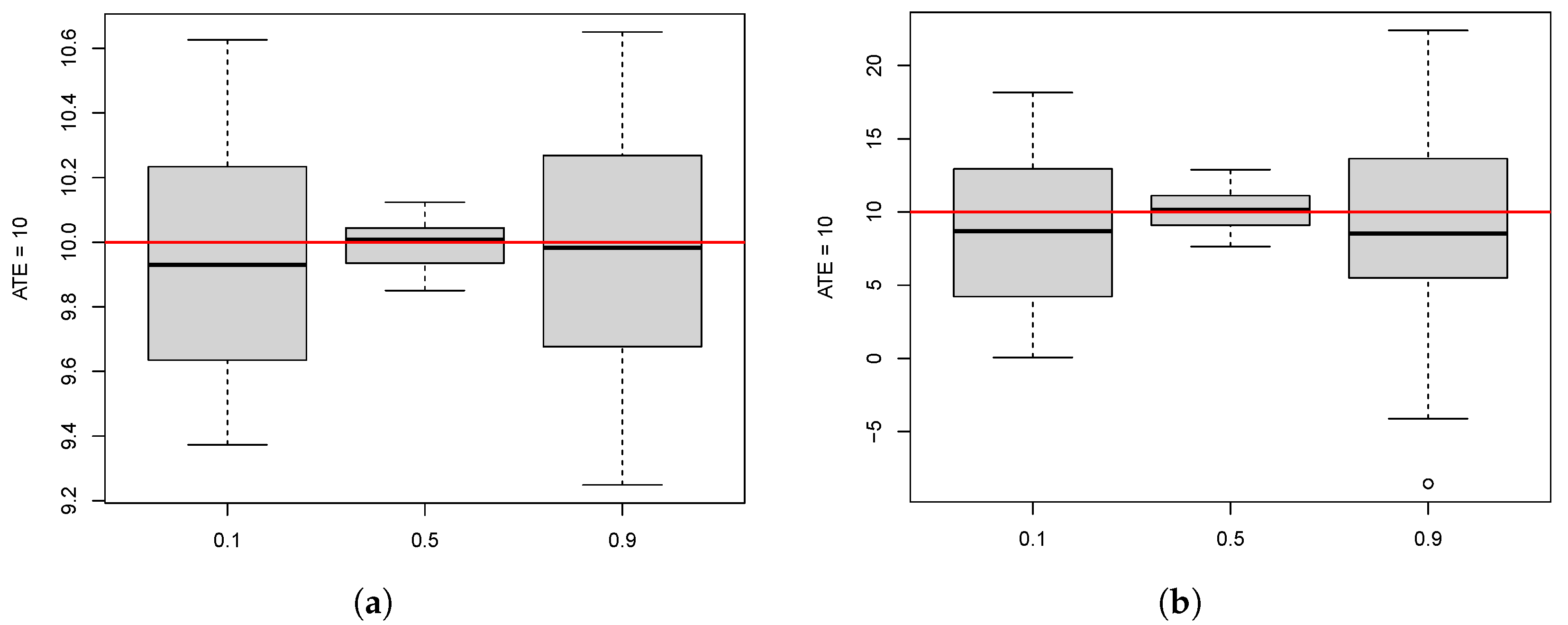
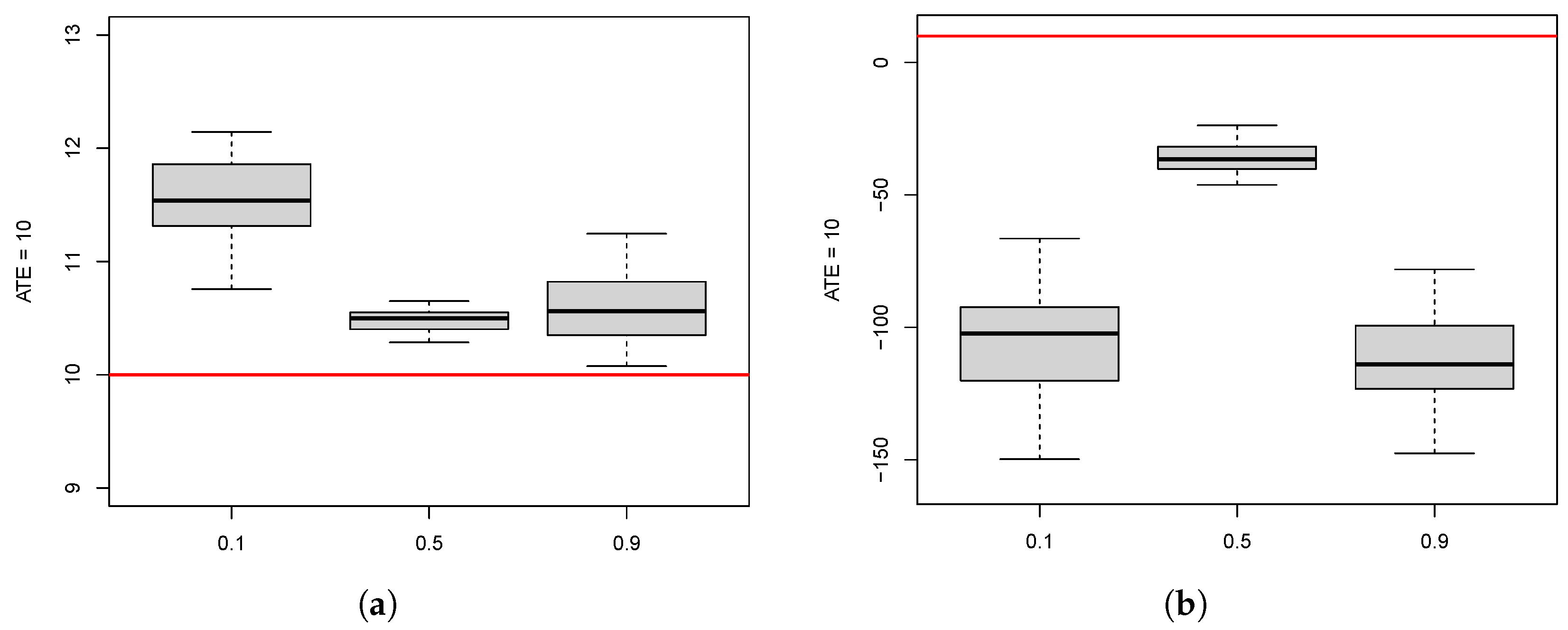
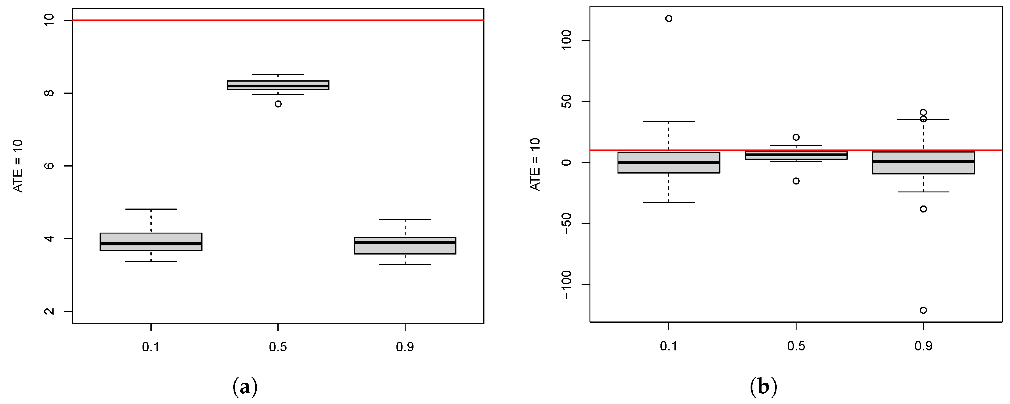
| Name | Description | Distribution |
|---|---|---|
| Grades A | Normal, = 50, sd = 5 | |
| Age | Normal, = 20, sd = 2 (minimum of 18) | |
| Grades B | Normal, = 45, sd = 6 | |
| Gender | Binomial, prob = 0.6 | |
| Bursary | Binomial, prob = 0.3 | |
| Grades C | Normal, = 70, sd = 7 | |
| T | Treatment | see Equation (4) |
| Method | Mean | SD | p-Value |
|---|---|---|---|
| Naive | 43.0 | 19.9 | 0.00 |
| Reg | 50.0 | 0.06 | 1.28 |
| LM | 49.9 | 1.62 | 0.98 |
| Lasso | 51.0 | 0.11 | 0.00 |
| RF | 48.1 | 0.14 | 0.00 |
| Method | Mean | SD | p-Value |
|---|---|---|---|
| Naive | 43.6 | 22.8 | 0.09 |
| Reg | 50.5 | 1.74 | 0.10 |
| LM | 50.0 | 1.66 | 0.10 |
| Lasso | 5.04 | 5.32 | 0.00 |
| RF | 44.1 | 0.14 | 0.00 |
Disclaimer/Publisher’s Note: The statements, opinions and data contained in all publications are solely those of the individual author(s) and contributor(s) and not of MDPI and/or the editor(s). MDPI and/or the editor(s) disclaim responsibility for any injury to people or property resulting from any ideas, methods, instructions or products referred to in the content. |
© 2023 by the authors. Licensee MDPI, Basel, Switzerland. This article is an open access article distributed under the terms and conditions of the Creative Commons Attribution (CC BY) license (https://creativecommons.org/licenses/by/4.0/).
Share and Cite
Smith, B.I.; Chimedza, C.; Bührmann, J.H. Treatment Effect Performance of the X-Learner in the Presence of Confounding and Non-Linearity. Math. Comput. Appl. 2023, 28, 32. https://doi.org/10.3390/mca28020032
Smith BI, Chimedza C, Bührmann JH. Treatment Effect Performance of the X-Learner in the Presence of Confounding and Non-Linearity. Mathematical and Computational Applications. 2023; 28(2):32. https://doi.org/10.3390/mca28020032
Chicago/Turabian StyleSmith, Bevan I., Charles Chimedza, and Jacoba H. Bührmann. 2023. "Treatment Effect Performance of the X-Learner in the Presence of Confounding and Non-Linearity" Mathematical and Computational Applications 28, no. 2: 32. https://doi.org/10.3390/mca28020032
APA StyleSmith, B. I., Chimedza, C., & Bührmann, J. H. (2023). Treatment Effect Performance of the X-Learner in the Presence of Confounding and Non-Linearity. Mathematical and Computational Applications, 28(2), 32. https://doi.org/10.3390/mca28020032


