3.1. Two-Dimensional Bending Actuators with ESP
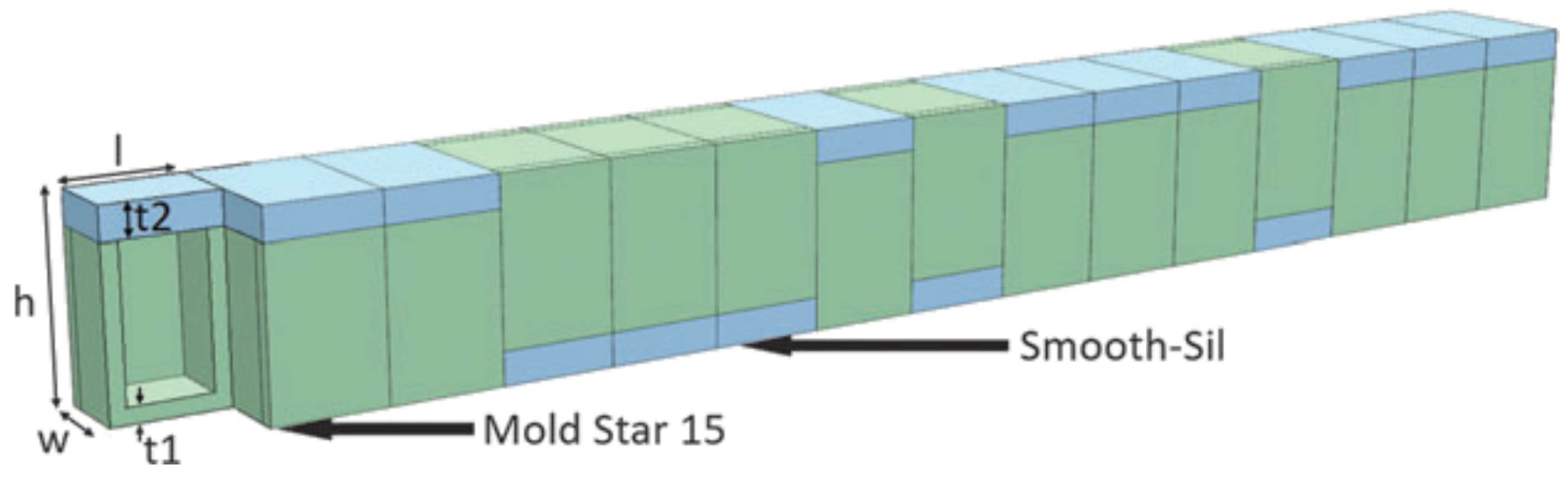
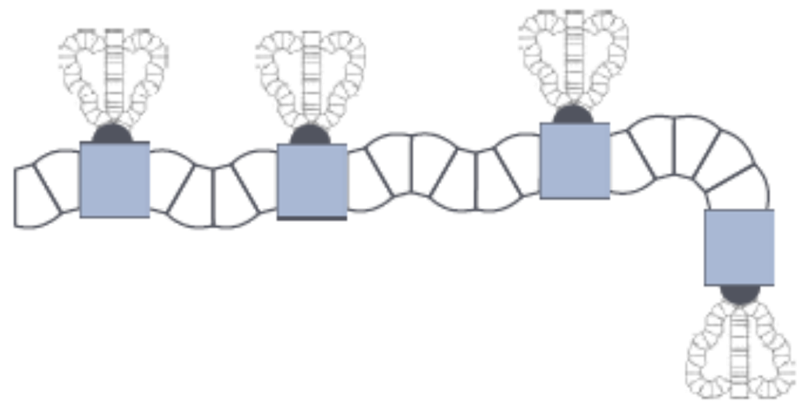
Ellis et al. assemble 15 identical bending units in either the up (↑) or down (↓) position to target one of four cases using a GA. For reference, the length of the assembled bending actuator is shown in
Figure 2 as the horizontal direction (
x), with increasing magnitude moving from left to right with a fully clamped condition representing
on the left end of the actuator. The vertical direction (
y) is perpendicular to the horizontal with
also at the centre of the clamped left edge of the actuator. Ellis et al. [
24] investigates four target cases,
Table 6, when a bending actuator is subjected to a given internal pressure.
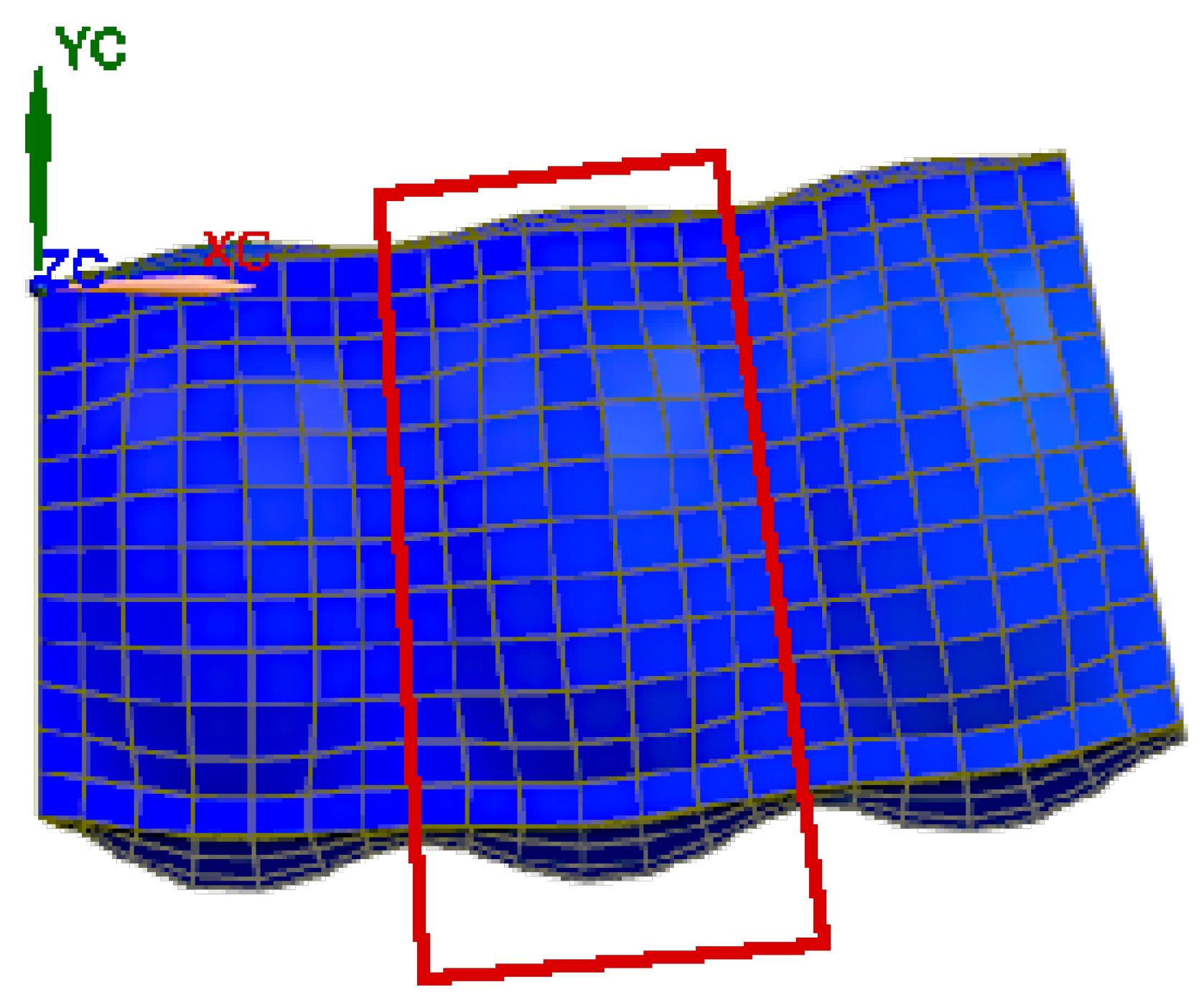
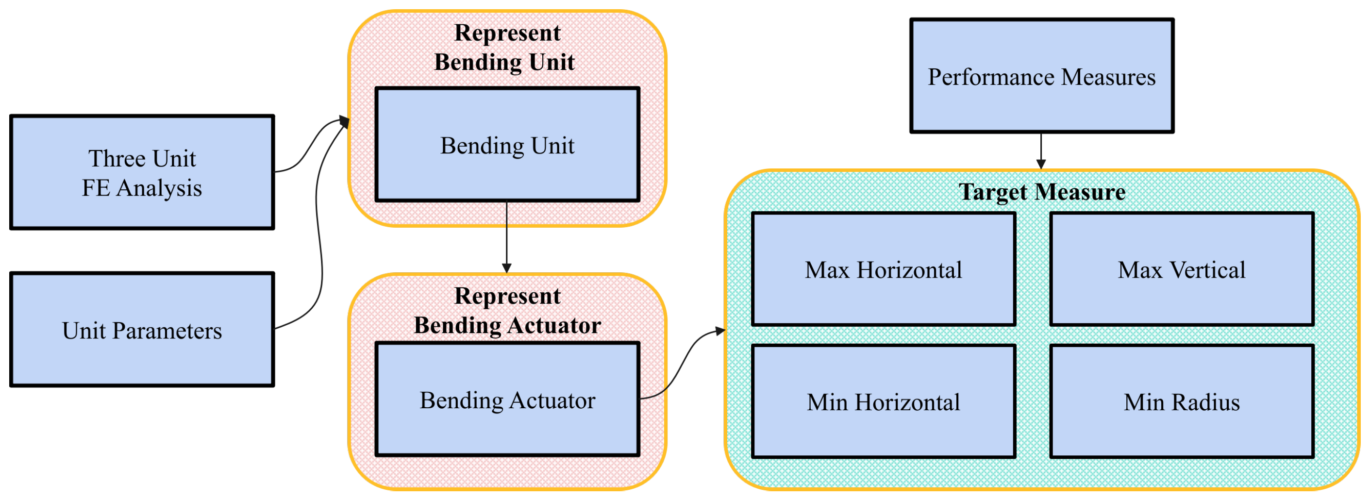
Figure 7 shows our approach using the ESP framework. Here we start with two encapsulations that represent pre-built modules used in later training. These two encapsulations are a parametric FE model of a three-unit bending actuator (three-unit FE analysis) and a dataset containing the ranges for each parameter in a single unit (Unit Parameters). These encapsulations are somewhat independent and can be swapped for encapsulations with similar properties easily. However, they represent a necessary starting position and tools that are not learnt within the ESP syllabus in this case. The syllabus consists of three modules, “represent bending unit”, “represent bending actuator” and “target measure”. The “represent bending unit” module is tasked with learning the bending response of a single bending unit within the parameter range contained within defined parameter ranges, using the method described in
Section 2.3, resulting in a model of a single bending unit (bending unit). The “represent bending actuator” module learns how to assemble the bending units into a predicted performance for a full actuator (bending actuator). The “target measure” module consists of learning the best configurations for each of the four target measures. For this, we need an encapsulation containing the definitions for the desired performance measures (performance measures).
This paper replicates the unit orientation results of Ellis et al., as shown in
Table 7. We further show that if we reverse each unit in the four results, there is a second viable configuration for each case, something not shown in Ellis’s work. Finally,
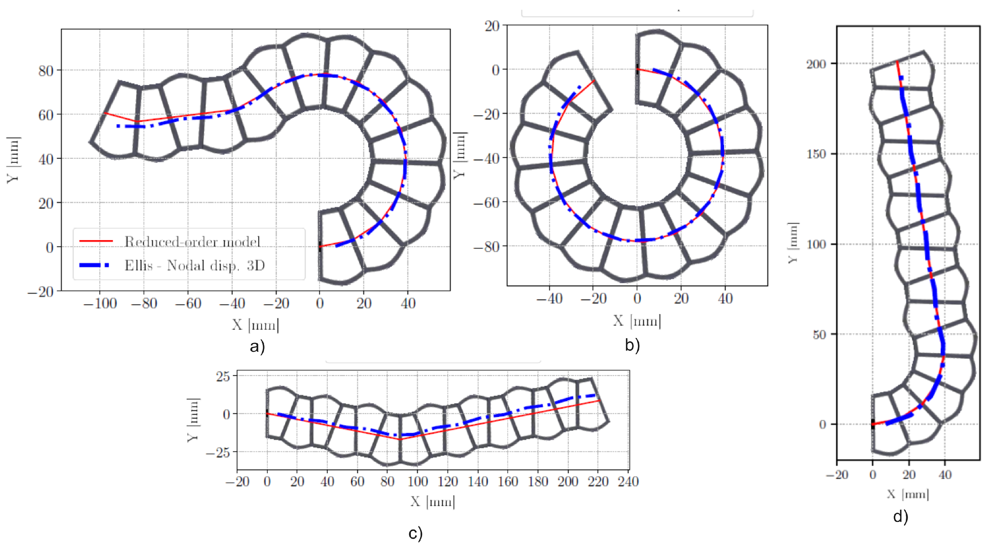
Table 8 compares the tip displacement measured and simulated by Ellis et al. with those found using ESP. In each case, the results of the ESP method proposed here show close conformance to those previously presented, as visually confirmed in
Figure 8. It is important to note that by making use of the pre-trained reduced order models resulting from the “Three Unit FEA” and “Unit Parameters” encapsulations, the optimisation time for each of the four target measures in the “Target Measure” module takes less than 1
compared to a single function evaluation using Ellis et al.’s reduced-order model taking around 45
on the same hardware. A single function evaluation of the “Three Unit FE Analysis” encapsulation used in training takes around 40
.
3.2. Multi-Gripper Tentacle with ESP
In
Section 3.1, we frame an established design problem within the ESP framework and found that in conjunction with the reduced-order model proposed in
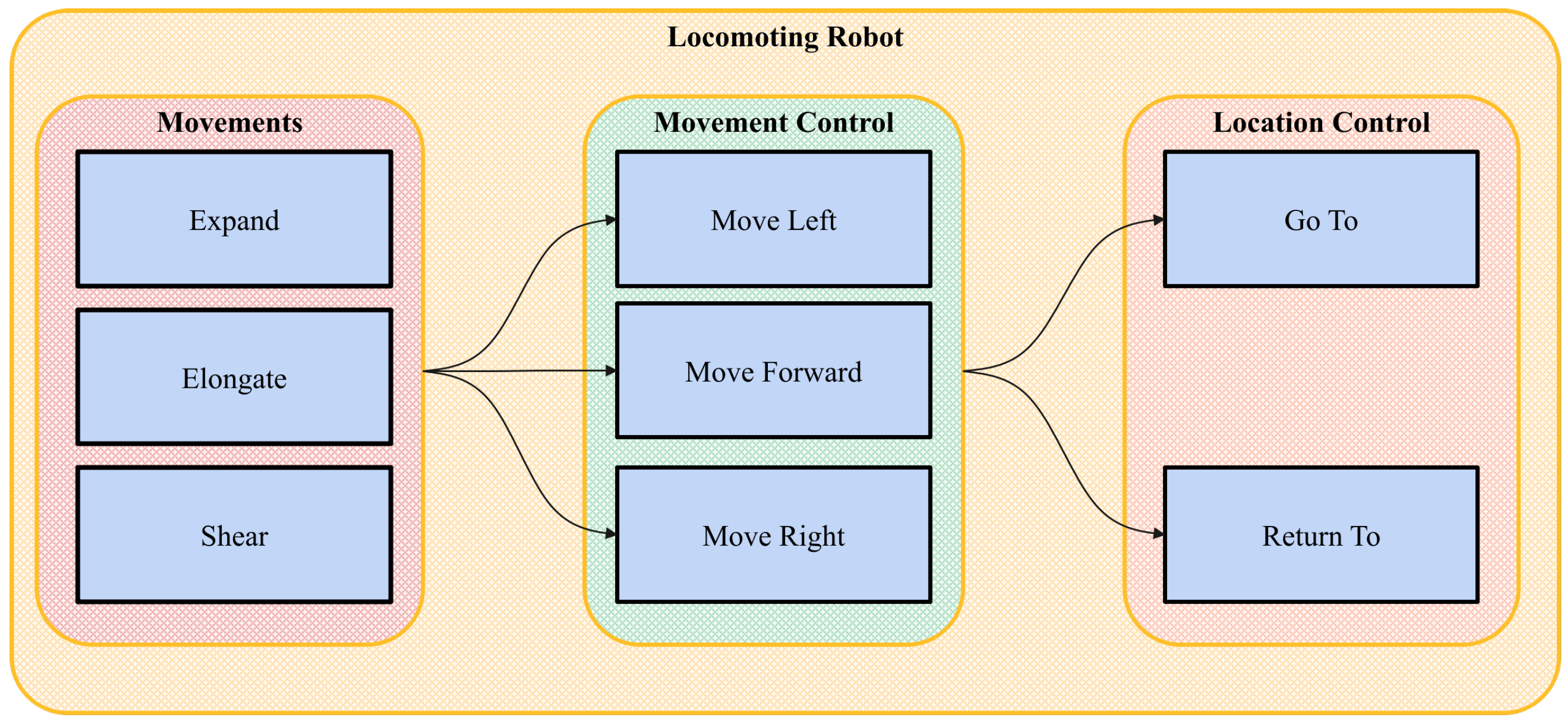
Section 2.3, we achieve comparable results in less time compared to using GA and FE simulations on their own. We now aim to use the ESP framework to create a tentacle-like soft robot that can articulate and grip multiple objects.
We have already constructed two useful encapsulations, (bending unit) and (bending actuator) in
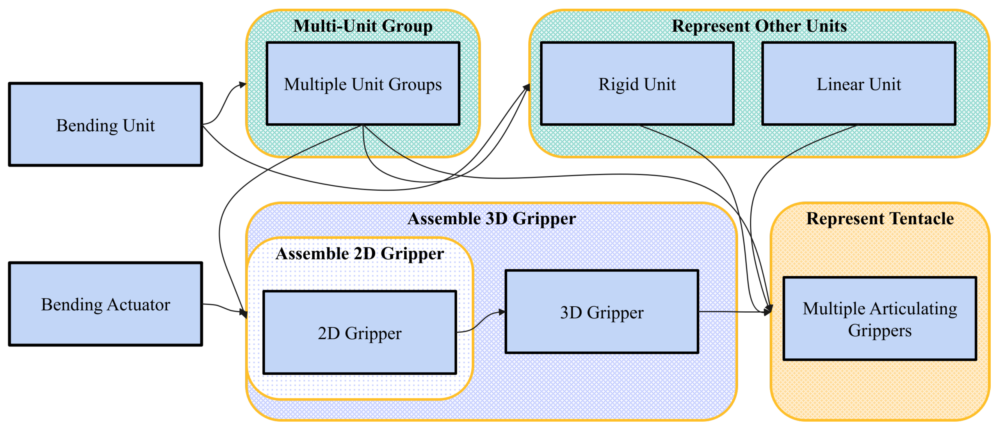
Section 3.1 that generate the response of various bending units and predict the behaviour of various bending unit assemblies. Since these are already trained and self-contained, we can simply use them in this project. To advance from these building blocks to a full tentacle, we have divided the design task into learning modules, as shown in
Figure 9.
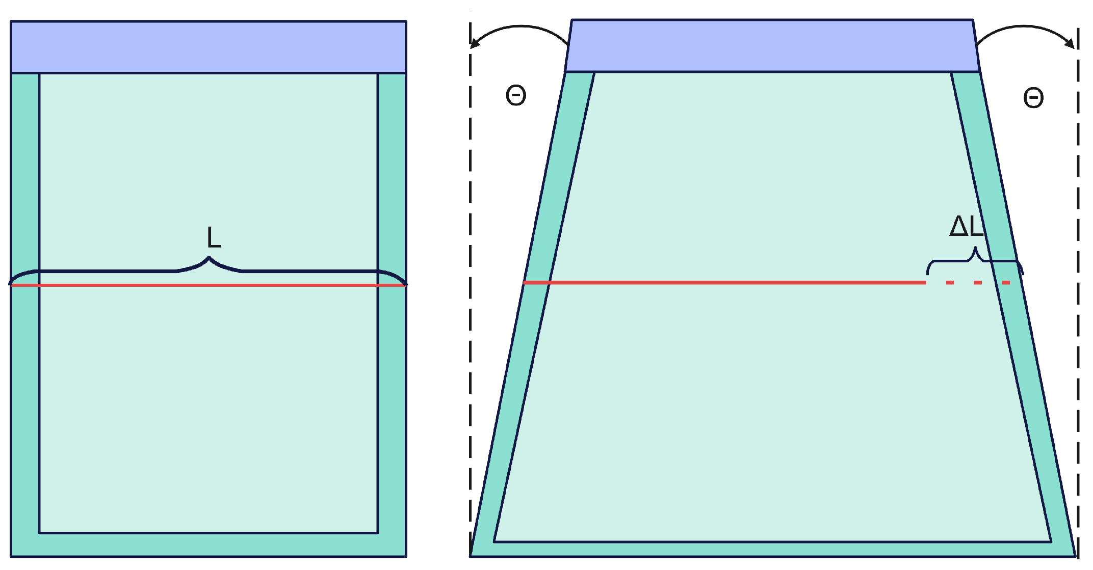
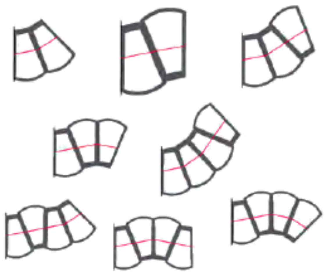
We know that some combinations of single units produce a cumulative effect different from that of a single unit. For example, a pressurised single unit forms a wedge shape. In contrast, a sequence of wedged units with the same orientation causes the assembly to curl, and a sequence of units with alternating orientation causes linear displacement. The “Multi-Unit Group” module explores and identifies unique combinations of units that produce alternate behaviours, such as a shallower bending angle, or no bending at all. These (multiple-unit groups) are not fully functional actuators but rather a larger pool of primitive components.
In the “multi-unit group” module, we use MCMC methods described in
Section 2.5 to explore and identify unique combinations of single units. Our objective is to find unique accumulations of tip displacement (
) and bending angle (
). We normalised the response of the multi-unit groups by the number of units in the assembly to favour smaller groups. This process combines elements of classification and selection, as we are generating a list of assemblies that perform a given displacement while acknowledging that multiple variations produce similar cumulative results. The resulting multiple-unit groups are then encapsulated as primitive components with their own behaviour for later modules.
Figure 10 shows a few examples of multiple-unit groups. It is important to note the stochastic nature of the process does not guarantee the same number of groups every time the algorithm runs or that the same groups will be found. This is in no way detrimental to the design process as the groups are potential options for later encapsulations.
The “Assemble 3D Gripper” combines the 2D Grippers learnt in the nested “Assemble 2D Gripper” module to produce a 3D Gripper capable of lifting volumetric objects. Here we use a nested module rather than two sequential modules to improve the reusability of the “Assemble 3D Gripper” module in later syllabi by including the ability to learn its own components rather than being limited to simply assembling previously generated elements.
In the “Assemble 2D Gripper” module, we learn how to assemble units and multi-unit groups to wrap around various 2D shapes. We start with the idea that construction follows a somewhat biological growth model, which can be easily scaled depending on the application. This means that a gripper well suited to gripping circles should look much the same regardless of the circles’ size. We begin with a simplified 2D case, encapsulating the gripper designs suitable for whichever object shape. Then, we use these 2D Grippers as elements in a higher-level encapsulation to generate 3D Gripper encapsulations.
With efficient access to encapsulated single and multi-unit groups, we can start targeting various profiles to be gripped. We use L-Systems, discussed in
Section 2.4, to learn an encoding for recursively generating scale-invariant assemblies that meet our objective of gripping an object in a particular state. For simplicity, we have a fixed starting point and assume the actuator lies in a straight line when noninflated.
Table 9 shows the L-system constructed to produce candidate 2D grippers. Here we again use a GA to learn the optimal production rules for a given target shape. The GA can replace any three-letter encoding with between four and ten randomly selected encodings and orientation symbols from the alphabet (shown as wildcard *).
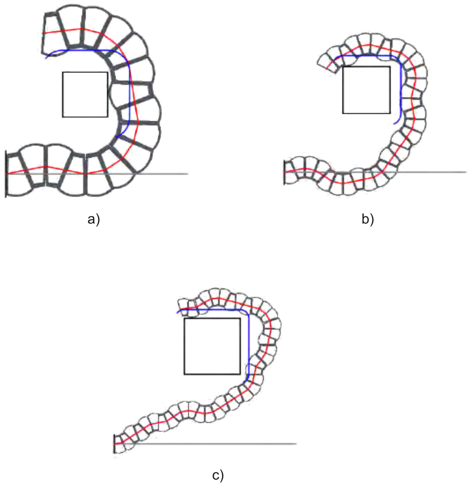
As target shapes, we generated circles, triangles, and squares at various distances from the starting point and created an offset shape half the height of the first unit away. We then made use of this offset shape as our target curve. If we can approximate the target shape with our bending actuator, we consider this to have “gripped” the shape.
Figure 11 shows the results of this gripper design process for three square targets at three distances and scales, using the same learnt L-system. Take note of the geometric similarity of the generated actuator at each scale.
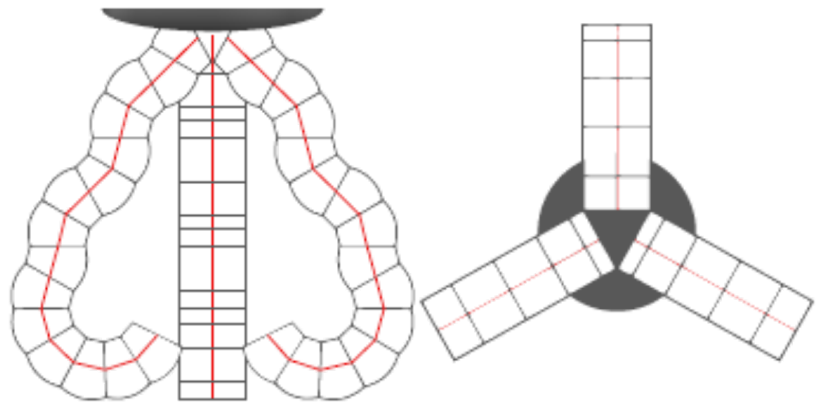
As you can see, the curve matching is imperfect, but the square is sufficiently surrounded to be considered “gripped”. This is an excellent example of how the designer is involved with decision-making through the ESP process. If the designer is satisfied with the results of a given encapsulation, they are free to use it in later modules. The 2D “gripper” is extended to the 3D case with a simple encapsulation, including a rigid centre and the option to attach
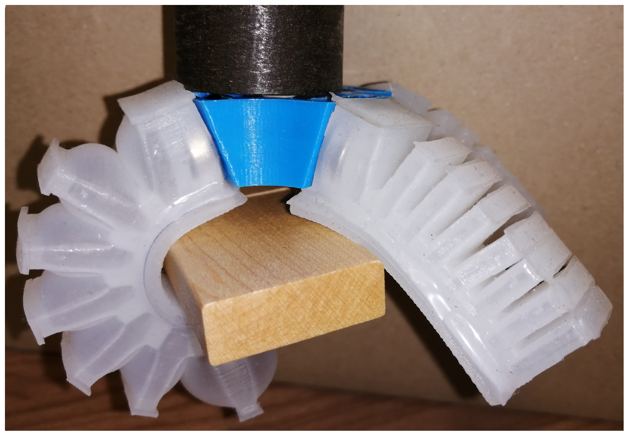
n 2D grippers radially about the periphery of the rigid centre. Simply testing a few variants leads to an encapsulation of three gripper units spaced 120° apart, as shown in
Figure 12.
Before we attempted to generate the full tentacle, we saw a need to include a few additional actuator options and created a “represent other units” module to learn a rigid unit and linear unit. Finally, in the last module, “represent tentacle”, we combine all earlier encapsulations to solve the overall design task of generating an actuating tentacle with multiple grippers, as shown in
Figure 13. Producing this design using the knowledge encapsulation produced in the first case study means that this result was produced in less than 30
. An advantage of the divide-and-conquer approach of ESP is that various methods can be used to accomplish each encapsulation task.


