Investigating the Surrogate Modeling Capabilities of Continuous Time Echo State Networks

Abstract

Continuous Time Echo State Networks (CTESNs) are a promising yet under-explored surrogate modeling technique for dynamical systems, particularly those governed by stiff Ordinary Differential Equations (ODEs). A key determinant of the generalization accuracy of a CTESN surrogate is the method of projecting the reservoir state to the output. This paper shows that of the two common projection methods (linear and nonlinear), the surrogates developed via the nonlinear projection consistently outperform those developed via the linear method. CTESN surrogates are developed for several challenging benchmark cases governed by stiff ODEs, and for each case, the performance of the linear and nonlinear projections is compared. The results of this paper demonstrate the applicability of CTESNs to a variety of problems while serving as a reference for important algorithmic and hyper-parameter choices for CTESNs.

1. Introduction

Modeling dynamic systems using scientific machine learning (SciML) techniques is a rapidly growing field with advanced ML architectures being applied to model complex problems across a diverse range of applications. Some examples are rapid design optimization [1], real-time health monitoring [2], turbulent flow modeling [3], and materials discovery [4]. Many of these applications utilize a “surrogate model” that makes real-time predictions of the system behavior in place of full-order models that would be too slow or expensive for the application.

Recently, Echo State Networks (ESNs) have seen an increase in popularity for modeling highly nonlinear and chaotic phenomena in domains such as optimal control planning [5], chaotic time series prediction [6,7], signals analysis [8] and even turbulent fluid flow [9]. These applications leverage the ability of ESNs to capture highly nonlinear transient behavior accurately, as well as the extremely low cost of training them, with the empirical success of ESNs on a wide range of approximation tasks discussed and explained in several works [10,11]. One of the biggest limitations, however, for using the standard ESN implementation in the surrogate modeling of nonlinear dynamical systems is that the available training data may not be uniformly sampled in time. A particular example of this is the numerical solution of stiff systems of Ordinary Differential Equations (ODEs) from ODE solvers. An ODE system is said to be stiff if, for any initial conditions and in certain intervals, the solving numerical method is forced to use a timestep which is very small compared to the smoothness of the exact solution [12]. Numerical ODE solvers overcome the instability due to stiffness by having a variable timestep size during the solve, leading to uneven sampling of the solution in time.

There have been several attempts to apply reduced-order modeling for stiff ODEs. Ji et al. [13] used Physics Informed Neural Networks [14], Kim et al. [15] used Neural ODEs [16], and Goswami et al. [17] used Deep Operator Networks [18] to solve several stiff systems such as the ROBER [19] and POLLU [20] problems. However, the methodologies applied require assumptions and scalings that may not generalize, or require many training data and computational resources to train deep neural networks. Work by Anantharaman et al. [21] also showed the failure of popular architectures such as Long Short-Term Memory (LSTM) and standard ESNs in modeling stiff systems.

To use the attractive properties of ESNs (i.e., capacity to model highly nonlinear signals and ease of training) for modeling stiff systems and to address this issue, a variant of ESNs called Continuous Time Echo State Networks or CTESNs has been proposed [21]. CTESNs have been successfully employed in various applications from accelerating predictions of power system dynamics [22] to accelerating solutions of pharmacology models [23].

In the recent literature, two ways of using CTESNs for surrogate modeling have emerged, the Linear Projection CTESN (LPCTESN) [21] and the Nonlinear Projection CTESN (NLPCTESN) [22,23], and these have been applied to a range of problems. However, there is currently a lack of work critically examining the accuracy of both methods and how they compare to one another. Further, both projection methods use a radial basis function (RBF) for interpolation, which also comes with several algorithmic choices that need to be explored. This study aims to fill this gap by investigating the effects of these algorithmic choices on surrogates created to solve several stiff ODE systems such as Robertson’s equations, the Sliding Basepoint model of automobile collision, and the POLLU air pollution model. The findings of the study show that for the same hyper-parameter settings of the CTESN, the NLPCTESN outperforms the LPCTESN on all benchmarks shown. Further, it is shown that for the interpolating RBFs used within CTESNs, k-Nearest Neighbor (k-NN) polynomial-augmented RBFs outperform standard RBFs in predictive accuracy.

This paper is divided as follows: Section 2 introduces the concept of ESN and CTESN, along with the projection methods LPCTESN and NLPCTESN described above discussed in detail. Section 3 demonstrates the application of the methods to several challenging stiff ODE problems, with a qualitative and quantitative discussion of the results. Section 4 summarizes the work with possible future directions to take.

2. Methods

2.1. Standard Echo State Networks

An Echo State Network [24], depicted in Figure 1, is a form of reservoir computing that is very similar to the more popular Recurrent Neural Network (RNN) in its architecture. It makes predictions by following a recurrence relation (Equation (1)) for updating a latent space vector and using that vector to map to a given output. Unlike RNNs, the parameters of the RNN in the “reservoir” are fixed and are not updated during training, and it is only the mapping from latent space to the output space that is learned. Depending on the implementation, this makes the training of ESNs very fast (sometimes as fast as a simple least squares fit) and computationally cheap.

The governing equation for an Echo State Network reads:

$${\mathbf{r}}_{n+1}=\sigma ({\mathbf{W}}_{in}{\mathbf{x}}_n+\mathbf{W}{\mathbf{r}}_n),$$

(1)

where ${\mathbf{r}}_n\in {\mathbb{R}}^{N_r}$ is the latent state at timestep n, $\sigma$ is an activation function (most commonly tanh), ${\mathbf{W}}_{in}\in {\mathbb{R}}^{N_r\times N_x}$ and $\mathbf{W}\in {\mathbb{R}}^{N_r\times N_r}$ are the reservoir matrices which are fixed and randomly initialized, and $x_n$ is the system state at time n. The matrix W is a sparse matrix and usually has 1% nonzero entries.

The output projection reads:

$${\mathbf{x}}_{n+1}=\Phi \left({\mathbf{r}}_{n+1}\right),$$

(2)

where $\Phi$ is decided by the projection method. The most popular projection method is the linear projection, resulting in

$${\mathbf{x}}_{n+1}={\mathbf{W}}_{out}{\mathbf{r}}_{n+1},$$

(3)

where ${\mathbf{W}}_{out}\in {\mathbb{R}}^{N_x\times N_r}$ is the linear projection matrix that needs to be fitted to the training data. Like most machine learning algorithms, ESNs have a set of hyper-parameters that need to be tuned, and there are several works [25,26] that can be used as guides to select them. A key hyper-parameter in ESNs is the spectral radius of $\mathbf{W}$. In this study, the spectral radius is fixed to a value of 0.01 for all models created. This value was obtained via a hyper-parameter search, details of which are given in Appendix C. Although a bit smaller than the conventional values used in standard ESNs, it was found in this study on CTESNs that using the slightly smaller value maximized predictive accuracy while also ensuring the stability of the reservoir (r) solution.

To fit the trainable matrix, one only has to solve the ordinary linear least squares problem:

$$\begin{array}{c}\hfill \begin{array}{cc}\hfill \mathrm{If}X=[{\mathbf{x}}_1;{\mathbf{x}}_2;\dots ;{\mathbf{x}}_N]& \mathrm{and}R=[{\mathbf{r}}_1;{\mathbf{r}}_2;\dots ;{\mathbf{r}}_N]\mathrm{then}\hfill \\ \hfill {\mathbf{W}}_{out}& ={\left(R{R}^T\right)}^{-1}RX.\hfill \end{array}\end{array}$$

(4)

2.2. Continuous Time Echo State Networks (CTESNs)

Continuous Time Echo State Networks are a variant of ESNs that model time as a continuous rather than discrete quantity. The model equation for a CTESN is given by:

$$\dot{\mathbf{r}}=\sigma ({\mathbf{W}}_{in}\mathbf{x}+\mathbf{W}\mathbf{r}),$$

(5)

with all variables having the same definition as in the previous section. The projection equation reads:

$$\mathbf{x}=\Phi \left(\mathbf{r}\right).$$

(6)

As per the literature, there are two ways of modeling the relation between the latent space and the outputs [27]; one is the linear method (called Linear Projection CTESN or LPCTESN), described by:

$$\mathbf{x}={\mathbf{W}}_{out}\mathbf{r}.$$

(7)

The second method is the nonlinear method (called NonLinear Projection CTESN or NLPCTESN), where the projection $\Phi$ is a nonlinear mapping. Many possible functions can be used, but the literature on NLPCTESNs [22,27] currently uses standard radial basis functions (RBFs) to write the projection:

$$\mathbf{x}=\mathbf{RBF}\left(\mathbf{r}\right).$$

(8)

Surrogate Modeling via CTESNs

To create and use a surrogate model via the CTESN method, a few steps are followed. First, a Design of Experiments (DoE) space is created and N sample combinations of query parameters are drawn; call this set P = {$p_1,p_2\dots p_N$}. Each $p_i$ represents a set of conditions at which the ODE is solved and the surrogate is expected to capture the change in the solution due to changes in the value of $p_i$. Examples include the initial conditions (see Section 3.1.2 and Section 3.2), rate constants of the ODE (see Section 3.1.1 and Section 3.3), etc. The ODE is solved numerically at each $p_i\in$ P, to return the solution set Y = {${\mathbf{y}}_1,{\mathbf{y}}_2\dots {\mathbf{y}}_n$}, ${\mathbf{y}}_i\in {\mathbb{R}}^{N_x\times N_{ts}^i}$. A single parameter combination $p^{*}\in$ P is drawn at random, and the reservoir ODE (given by Equation (5)) is solved using a numerical ODE solver. This returns an r(t) $\in {\mathbb{R}}^{N_r\times N_{ts}}$ where $N_{ts}$ is the number of timesteps in the solution at $p^{*}$. Then, depending on whether the method follows a linear or nonlinear projection method, either Algorithm 1 or Algorithm 2 is followed to fit and query the surrogate.

Algorithm 1 Linear Projection CTESN Surrogate Fitting

for ${\mathbf{y}}_i$ in Y do    Fit $W_{out}^i$ from ${\mathbf{y}}_i=W_{out}^i·$ r using Equation (4) end for Fit RBF mapping $W_{out}^i=\mathbf{RBF}\left(p_i\right),\forall$ ($W_{out}^i,p_i$) pairs To query a new parameter $p_{test}$:  Step 1: $W_{out}^{test}=\mathbf{RBF}\left(p_{test}\right)$  Step 2: ${\mathbf{y}}_{test}$(t) = $W_{out}^{test}·$r

Algorithm 2 NonLinear Projection CTESN Surrogate Fitting

for ${\mathbf{y}}_i$ in Y do    Fit ${\mathbf{RBF}}_1^i$ as per ${\mathbf{y}}_i={\mathbf{RBF}}_1^i(\mathbf{r}\left(t\right),{\mathbf{W}}_{RB{F}_1}^i)$ end for Fit ${\mathbf{RBF}}_2$ as per ${\mathbf{W}}_{RB{F}_1}^i={\mathrm{RBF}}_2\left(p_i\right)$, ∀$({\mathbf{W}}_{RB{F}_1}^i,p_i)$ pairs To query a new parameter $p_{test}$:  Step 1: $W_{RB{F}_1}^{test}={\mathbf{RBF}}_2\left(p_{test}\right)$  Step 2: ${\mathbf{y}}_{test}$(t) = ${\mathbf{RBF}}_1(W_{RB{F}_1}^{test},\mathbf{r}$(t))

Algorithms 1 and 2 both use an interpolating RBF in their procedure, and in this article, it is demonstrated that polynomial-augmented k-Nearest Neighbor (k-NN) RBFs deliver superior results in terms of generalization to new test problems for CTESN-based surrogate models, compared to standard RBFs. The reader is encouraged to read Appendix A for a detailed explanation of k-NN polynomial-augmented RBFs.

3. Applications and Results

CTESN surrogates are created for three problems. First, Robertson’s equations are solved, parametrizing the rates of reaction and initial condition separately. Then, the Sliding Basepoint system is modeled, comparing explicitly the difference due to the projection method and parametrizing the initial conditions of the problem. Finally, the POLLU system is solved, again parametrizing the initial conditions of the problem and comparing the results obtained using differing projection methods. Unless mentioned otherwise, the training data were sampled from the DoE space randomly.

In all results in this section, the MAE is computed as

$$\mathbf{MAE}=\frac{1}{N_{test}}\sum _{j=1}^{N_{test}}\frac{{\sum }_{i=1}^{N_{ts}^j}|y_{j,pred}^i-y_{j,true}^i|}{N_{ts}^j},$$

(9)

where $N_{test}$ is the number of test cases; $y_{j,pred}^i$ and $y_{j,true}^i$ are the prediction and true solution, respectively, for the ith timestep of the jth test case.

3.1. Robertson’s Equations

The first demonstrated application is the surrogate modeling of the Robertson Equations [19]. They are written as:

$$\begin{array}{c}\hfill \begin{array}{cc}\hfill \dot{y_1}& =-r_1·y_1+r_3·y_2·y_3,\hfill \\ \hfill \dot{y_2}& =r_1·y_1-r_3·y_2·y_3-r_2·y_2^2,\hfill \\ \hfill \dot{y_3}& =r_2·y_2^2,\hfill \end{array}\end{array}$$

(10)

where $y_1,y_2$, and $y_3$ represent the concentration of the reactant species and $r_1,r_2$, and $r_3$ represent the fixed rates of reaction. The system is usually subject to initial conditions of $[y_1,y_2,y_3]=[1,0,0]$.

They are a system of ODEs that describe a standard rate process and are often used to benchmark numerical ODE solvers due to the stiffness of the system. More specifically, the long-time integration of Robertson’s equations is known to be a challenging problem for numerical ODE solvers, and the system hence serves as a good test for surrogate models. In this work, models are created by parametrizing the system in two ways; first, the rates of reaction are parametrized. This has been the focus of several other papers written on CTESNs [21,27]. Second, the initial conditions of the system are parametrized.

3.1.1. Parametrizing Rates of Reaction

In this section, the Design of Experiment (DoE) space for the rates is given as:

$$\begin{array}{c}\hfill \begin{array}{cc}\hfill r_1& =[0.032,0.048],\hfill \\ \hfill r_2& =[2.4,3.6]\times E7,\hfill \\ \hfill r_3& =[0.8,1.2]\times E4.\hfill \end{array}\end{array}$$

(11)

The focus is limited to presenting the results of the prediction of the variable $y_2$. This variable has a sharp transient that occurs at a time scale much smaller than the other two, and hence causes the system to be stiff.

The average MAE for $y_2$, averaged across several test cases listed in

Table 1. Test parameter values for rate parametrization of Robertson’s ODE system.

Parameter Set	${\mathit{r}}_1/0.04$	${\mathit{r}}_2/3·\mathit{E}7$	${\mathit{r}}_3/1·\mathit{E}4$
P1	0.95	1.05	0.95
P2	0.9	1.1	0.9
P3	1.1	0.9	1.1
P4	1.03	0.99	1.04

, is shown in

Table 2. Average Mean Absolute Error (MAE) in $y_2$, averaged across all test cases.

Trial No.	${\mathbf{N}}_{\mathit{r}}$	${\mathbf{N}}_{\mathit{data}}$	${\mathbf{N}}_{\mathit{neigh}}$	Polynomial Augmentation	Projection Method	Avg. MAE ($\times {\mathbf{10}}^{-\mathbf{7}}$)
1	50	50	4	N	Linear	17.6
2	50	50	All	Y	Linear	1.40
3	50	500	4	Y	Linear	1.29
4	50	50	4	Y	Linear	0.76
5	50	50	4	Y	Nonlinear	0.32

sorted in descending order of generalization MAE. Predictions for $y_2$ for a particular test parameter are shown in Figure 2. For the same hyper-parameters, it can be observed that the absence of either the augmenting polynomial or the k-NN interpolation (i.e., using all collocation points to predict the solution in the RBF) significantly increases the error of prediction. It can also be seen that the nonlinear projection performs better on average than the linear projection.

In the next section, the initial condition of Robertson’s ODE is parametrized, and a similar error analysis is performed.

3.1.2. Parametrizing Initial Conditions

The initial condition of the system is parametrized. This problem can be challenging for lower initial values of $y_1$(0) as it leads to a smaller and sharper transient in $y_2$, which becomes more difficult to capture accurately by the surrogate. The DoE space of the initial condition is given as

$$\begin{array}{c}\hfill \begin{array}{cc}\hfill y_1\left(0\right)& =[0.5,1],\hfill \\ \hfill y_2\left(0\right)& =0,\hfill \\ \hfill y_3\left(0\right)& =1-y_1\left(0\right).\hfill \end{array}\end{array}$$

(12)

The condition for $y_3$ is decided on the basis that the sum of all quantities should always equal to 1. Once more, the focus is on comparing the predicted results in $y_2$.

Table 3. Average Mean Absolute Error (MAE) in $y_2$, averaged across all test cases when parametrizing the initial condition.

Trial No.	${\mathbf{N}}_{\mathit{r}}$	${\mathbf{N}}_{\mathit{data}}$	${\mathbf{N}}_{\mathit{neigh}}$	Projection Method	Avg. MAE ($\times {\mathbf{10}}^{-\mathbf{7}}$)
1	500	50	All	Linear	158
2	50	50	All	Linear	28.6
3	500	50	4	Linear	25.2
4	50	50	4	Linear	6.23
5	50	50	4	Nonlinear	0.99

tabulates the average MAE across all test cases for the problem, listed in

Table 4. Test parameter values for initial condition parametrization of Robertson’s ODE system.

Parameter Set	${\mathit{y}}_1$	${\mathit{y}}_2$	${\mathit{y}}_3$
P1	0.6	0	0.4
P2	0.7	0	0.3
P3	0.85	0	0.15
P4	0.9	0	0.1

, sorted in descending order. Figure 3 shows the comparison for a test parameter, across five different configurations of the CTESN surrogate model. A similar trend of hyper-parameter performance as seen in Table 2 is noted, in that the absence of the k-NN interpolation increases the error of the prediction. For the same hyper-parameters, the nonlinear projection once again achieves lower generalization MAE than the linear projection.

3.2. Sliding Basepoint Model

Finally, the discussed methods are applied to the surrogate modeling of a realistic crash safety design problem. A system of ODEs proposed by Horváth et al. [28] that approximately models an automobile collision is solved via a created surrogate model. This system, called the Sliding Basepoint model, has parameters that were fitted on realistic crash data and are assumed to accurately model a collision problem. Figure 4 depicts the system at its initial state and at a later time. The system is given as:

$$\begin{array}{c}\hfill \begin{array}{cc}\hfill \dot{x_1}& =v_1,\hfill \\ \hfill \dot{v_1}& =\frac{1}{m_1}{F}_1(F_s,c_1,v_1),\hfill \\ \hfill \dot{x_2}& =v_2,\hfill \\ \hfill \dot{v_2}& =\frac{1}{m_2}{F}_2(-F_s,c_2,v_2),\hfill \\ \hfill \dot{k}& =D_k·P,\hfill \\ \hfill \dot{c_1}& =D_c·P,\hfill \end{array}\end{array}$$

(13)

where $m_1,m_2,F_1,F_2,x_1,x_2,v_1,v_2$ refer to the masses, total forces on, positions, and velocities of the bodies, respectively. $m_1$ in reality reflects the mass of the chassis of the car; $x_1$ behaves similarly to the deformation of the bumper. $F_s$ represents the spring force:

$$F_s=k·(x_2-x_1),$$

(14)

between the two masses and P represents the power of dissipation

$$P = |m_1·v_1^2|.$$

(15)

Finally, the forces are computed based on best-fit models described in the paper:

$$\begin{array}{c}\hfill \begin{array}{cc}\hfill F_1(F_s,c_1,v_1)& =F_s-c_1·\left|v_1\right|·sign\left(v_1\right),\hfill \\ \hfill F_2(F_s,c_2,v_2)& =\left\{\begin{array}{cc}0,\hfill & \mathrm{if}{F}_s<c_2\mathrm{or}\left|v_2\right|<v_f\hfill \\ F_s-c_2·sign\left(v_2\right),\hfill & \mathrm{otherwise}\hfill \end{array}\right.\hfill \end{array}\end{array}$$

(16)

The values of the fixed parameters are given in

Table 5. Parameter values taken from [28] with their SI units.

${\mathbf{m}}_1$ (kg)	${\mathbf{m}}_2$ (kg)	${\mathbf{D}}_{\mathit{k}}$	${\mathbf{D}}_{\mathit{c}}$	${\mathit{c}}_2$ (N)	${\mathit{v}}_{\mathit{f}}$ (m/s)
1916	24.9	3.38	0.459	145,000	0.1

, and the parameter values changed while testing the surrogate are listed in

Table 6. Test parameter values for the collision modeling problem.

Parameter Set	${\mathit{v}}_0/25$	${\mathit{k}}_0/{10}^6$
P1	0.496	4.46
P2	0.884	8.45
P3	0.424	1.43
P4	0.283	3.75
P5	0.9	9.95

. The reader is referred to the paper [28] for further details. The system is subject to initial conditions $[x_1,v_1,x_2,v_2,k,c_1]=[0,v_0,0,0,k_0,0]$.

The mechanics of crash and impact problems are known to have sharp transients and highly oscillatory behaviors associated with them, making their numerical solutions slow and costly to compute for a wide range of parameters. Hence, CTESNs will be a good surrogate modeling tool for the problem.

In this work, the initial conditions of the problem ($v_0$ and $k_0$) are parametrized to simulate different impact velocities and directions (the spring constant of the bumper can be assumed to be different in different directions). The state space for the problem is the vector $[x_1,v_1,x_2,v_2,k,c_1]$.

The DoE space is the range:

$$\begin{array}{c}\hfill \begin{array}{cc}\hfill {\mathrm{v}}_0& =[5,25](\mathrm{m}/\mathrm{s}),\hfill \\ \hfill {\mathrm{k}}_0& =[1,10]\times {10}^6\mathrm{kg}/s^2,\hfill \end{array}\end{array}$$

(17)

chosen to represent a wide range of speeds and stiffness constants. The DoE space was sampled using a space-filling sampling strategy [29] and the surrogate models were trained on 100 data points, and data were generated using a stiff ODE solver using solver parameters given in [28].

Table 7. Average Mean Absolute Error (MAE) in $v_2$, averaged across all test cases in Table 6.

Trial No.	${\mathbf{N}}_{\mathit{x}}$	${\mathbf{N}}_{\mathit{neigh}}$	Projection Method	Avg. MAE (${\mathit{v}}_2$)
1	50	4	Linear	1.02
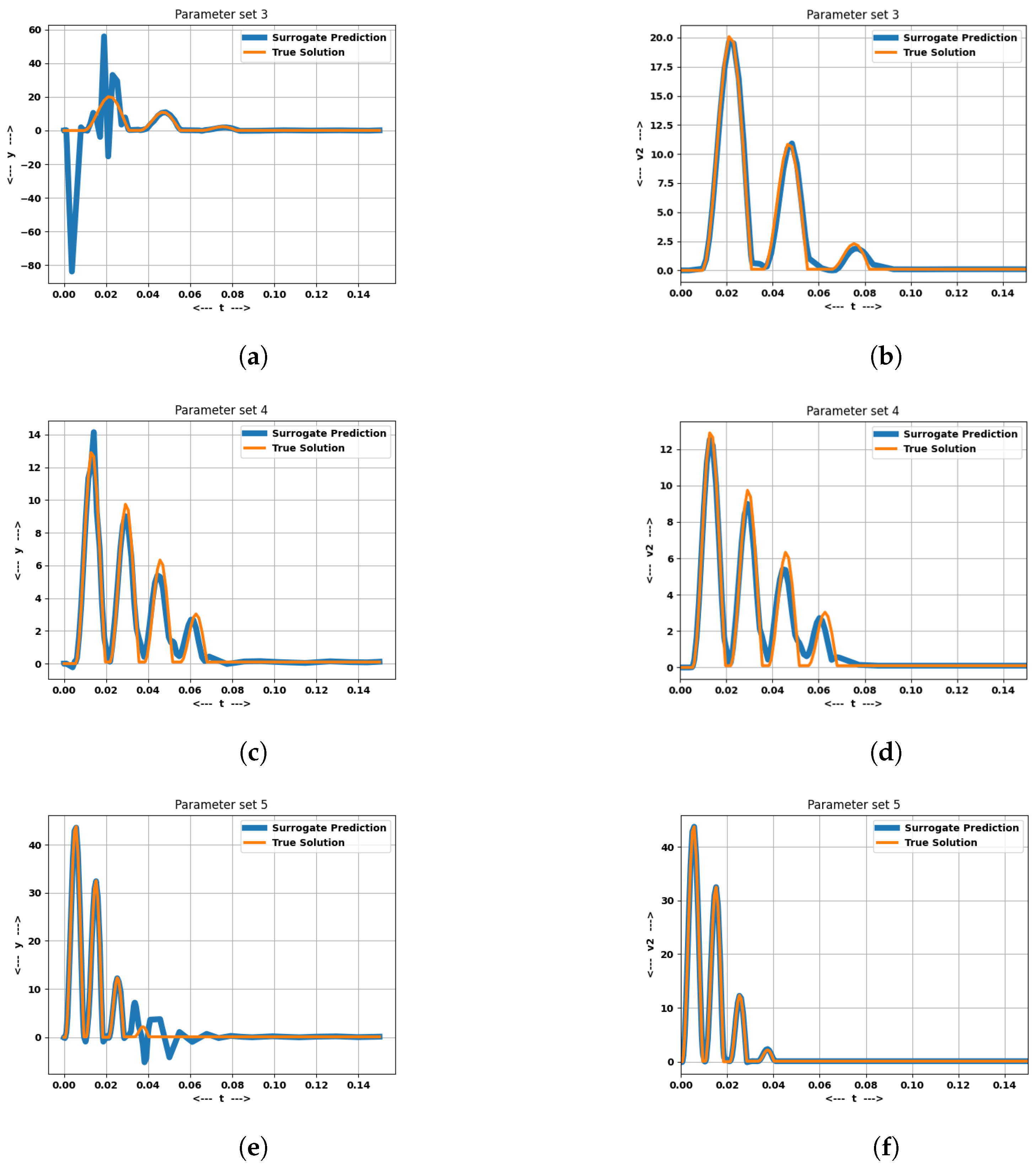
2	50	4	Nonlinear	0.51

shows the average MAE for the state variable $v_2$ for the linear and nonlinear projection methods, all other hyper-parameters being kept the same, for test parameters listed in Table 5. $v_2$ was chosen to demonstrate the accuracy of the surrogates because, as is visible in Figure 5, it has sharp nonlinear oscillatory transients starting from the moment of collision, which is difficult to capture for surrogate models. It can be seen from Table 7 and Figure 5 that the LPCTESN has a poorer performance on test cases compared to the NLPCTESN.

Of particular interest is the speedup obtained by using the surrogate; this leads to up to a 200× speedup in the prediction of the solution, the ODE solver taking roughly 0.02 s per solve of the ODE system. This is important because the transients in Figure 5 occur at the same time scale $\mathcal{O}\left({10}^{-2}s\right)$. With a 200× speedup, if the surrogate is deployed on board a vehicle, it can judge the severity of the collision much more quickly by computing impact forces from the result of the system, and closed-loop control and safety measures can be deployed. In this case, it would effectively function as a digital twin for collision monitoring.

3.3. The POLLU Model

The CTESN approach is used to model the POLLU air pollution model developed at the Dutch National Institute of Public Health and Environmental Protection [20]. It consists of 20 species and 25 reactions, modeled by nonlinear ODEs of the form

$$\frac{dy}{dt}=P(t,y)-L(t,y)y,$$

(18)

where y is the concentration vector (in ppm) of the reacting species, P is the production term, and L is a diagonal matrix representing the loss term for every species in the system.

Table 8. Species involved in the POLLU reaction system, with their production and loss rates, derived from [20].

Species (y)	Production Rate (P)	Loss Rate (L)
1	$$\begin{gathered} r_2{y}_2{y}_4+r_3{y}_5{y}_2+r_9{y}_{11}{y}_2+r_{11}{y}_{13} \\ \hspace{1em}\hspace{1em}{r}_{12}{y}_{10}{y}_2+r_{22}{y}_{19}+r_{25}{y}_{20} \end{gathered}$$	$$\begin{gathered} r_1+r_{10}{y}_{11}+r_{14}{y}_6 \\ \hspace{1em}{r}_{23}{y}_4+r_{24}{y}_{19} \end{gathered}$$
2	$r_1{y}_1+r_{21}{y}_{19}$	$r_2{y}_4+r_3{y}_5+r_9{y}_{11}+r_{12}{y}_{10}$
3	$r_1{y}_1+r_{17}{y}_5+r_{19}{y}_{16}+r_{22}{y}_{19}$	$r_{15}$
4	$r_{15}{y}_3$	$r_2{y}_2+r_{16}+r_{17}+r_{23}{y}_1$
5	$$\begin{gathered} r_4{y}_7+r_4{y}_7+r_6{y}_7{y}_6+r_7{y}_9 \\ \hspace{1em}\hspace{1em}{r}_{13}{y}_{14}+r_{20}{y}_{17}{y}_6 \end{gathered}$$	$r_3{y}_2$
6	$r_3{y}_5{y}_2+r_{18}{y}_{16}+r_{18}{y}_{16}$	$r_6{y}_7+r_8{y}_9+r_{14}{y}_1+r_{20}{y}_{17}$
7	$r_{13}{y}_{14}$	$r_4+r_5+r_6{y}_6$
8	$r_4{y}_7+r_5{y}_7+r_6{y}_7{y}_6+r_7{y}_9$	0.0
9	0	$r_7+r_8{y}_6$
10	$r_7{y}_9+r_9{y}_{11}{y}_2$	$r_{12}{y}_2$
11	$r_8{y}_9{y}_6+r_{11}{y}_{13}$	$r_9{y}_2+r_{10}{y}_1$
12	$r_9{y}_{11}{y}_2$	0.0
13	$r_{10}{y}_{11}{y}_1$	$r_{11}$
14	$r_{12}{y}_{10}{y}_2$	$r_{13}$
15	$r_{14}{y}_1{y}_6$	0.0
16	$r_{16}{y}_4$	$r_{18}+r_{19}$
17	0.0	$r_{20}{y}_6$
18	$r_{20}{y}_{17}{y}_6$	0.0
19	$r_{23}{y}_1{y}_4+r_{25}{y}_{20}$	$r_{21}+r_{22}+r_{24}{y}_1$
20	$r_{24}{y}_{19}{y}_1$	$r_{25}$

shows the production and loss rates for each species of the system. The values of the rate constants r are given in

Table A1. Reaction rates for the POLLU problem.

Reaction Rate	Value	Reaction Rate	Value
$r_1$	0.350 $\times {10}^0$	$r_{14}$	0.163 $\times {10}^5$
$r_2$	0.266 $\times {10}^2$	$r_{15}$	0.480 $\times {10}^7$
$r_3$	0.120 $\times {10}^5$	$r_{16}$	0.350 $\times {10}^{-3}$
$r_4$	0.860 $\times {10}^{-3}$	$r_{17}$	0.175 $\times {10}^{-1}$
$r_5$	0.820 $\times {10}^{-3}$	$r_{18}$	0.100 $\times {10}^9$
$r_6$	0.150 $\times {10}^5$	$r_{19}$	0.444 $\times {10}^{12}$
$r_7$	0.130 $\times {10}^{-3}$	$r_{20}$	0.124 $\times {10}^4$
$r_8$	0.240 $\times {10}^5$	$r_{21}$	0.210 $\times {10}^1$
$r_9$	0.165 $\times {10}^5$	$r_{22}$	0.578 $\times {10}^1$
$r_{10}$	0.900 $\times {10}^4$	$r_{23}$	0.474 $\times {10}^{-1}$
$r_{11}$	0.220 $\times {10}^{-1}$	$r_{24}$	0.178 $\times {10}^4$
$r_{12}$	0.120 $\times {10}^5$	$r_{25}$	0.312 $\times {10}^1$
$r_{13}$	0.188 $\times {10}^1$

. The reader is referred to the paper [20] for a complete description of the reaction system.

The system is a common benchmark for stiff ODE solvers and represents a difficult problem to solve due to the large number of species and ODEs involved. When such systems have to be solved at many grid points, say, in a computational mesh, they represent a very expensive computation and hence this example is an ideal application for testing surrogates of stiff ODEs. In this work, the initial conditions of the system are simultaneously parametrized, according to the following:

$$\begin{array}{c}\hfill \begin{array}{cc}\hfill {\mathrm{y}}_{2,0}& =[0.14,0.26],\hfill \\ \hfill {\mathrm{y}}_{4,0}& =[0.028,0.052],\hfill \\ \hfill {\mathrm{y}}_{7,0}& =[0.07,0.13].\hfill \end{array}\end{array}$$

(19)

Here, $y_{2,0}$, $y_{4,0}$, and $y_{7,0}$ refer to the initial concentration of the respective species. The initial conditions for the rest of the species are default as per the paper [20].

The training data were sampled using 100 data points within this DoE space, selected randomly. The reservoir size ${\mathbf{N}}_r$ was set to 100, and the number of queried neighbors ${\mathbf{N}}_{neigh}$ by the k-NN RBF was set to 10.

Table 9. Mean Absolute Error (MAE) for the POLLU problem, averaged across all test cases in Table 10.

Projection Method	Mean Absolute Error
	${\mathit{y}}_{\mathbf{1}}(\times {\mathbf{10}}^{-\mathbf{5}})$	${\mathit{y}}_{\mathbf{2}}(\times {\mathbf{10}}^{-\mathbf{5}})$	${\mathit{y}}_{\mathbf{4}}(\times {\mathbf{10}}^{-\mathbf{4}})$	${\mathit{y}}_{\mathbf{14}}(\times {\mathbf{10}}^{-\mathbf{8}})$	${\mathit{y}}_{\mathbf{20}}(\times {\mathbf{10}}^{-\mathbf{6}})$
Linear	75.1	76.3	7.68	51.5	22.1
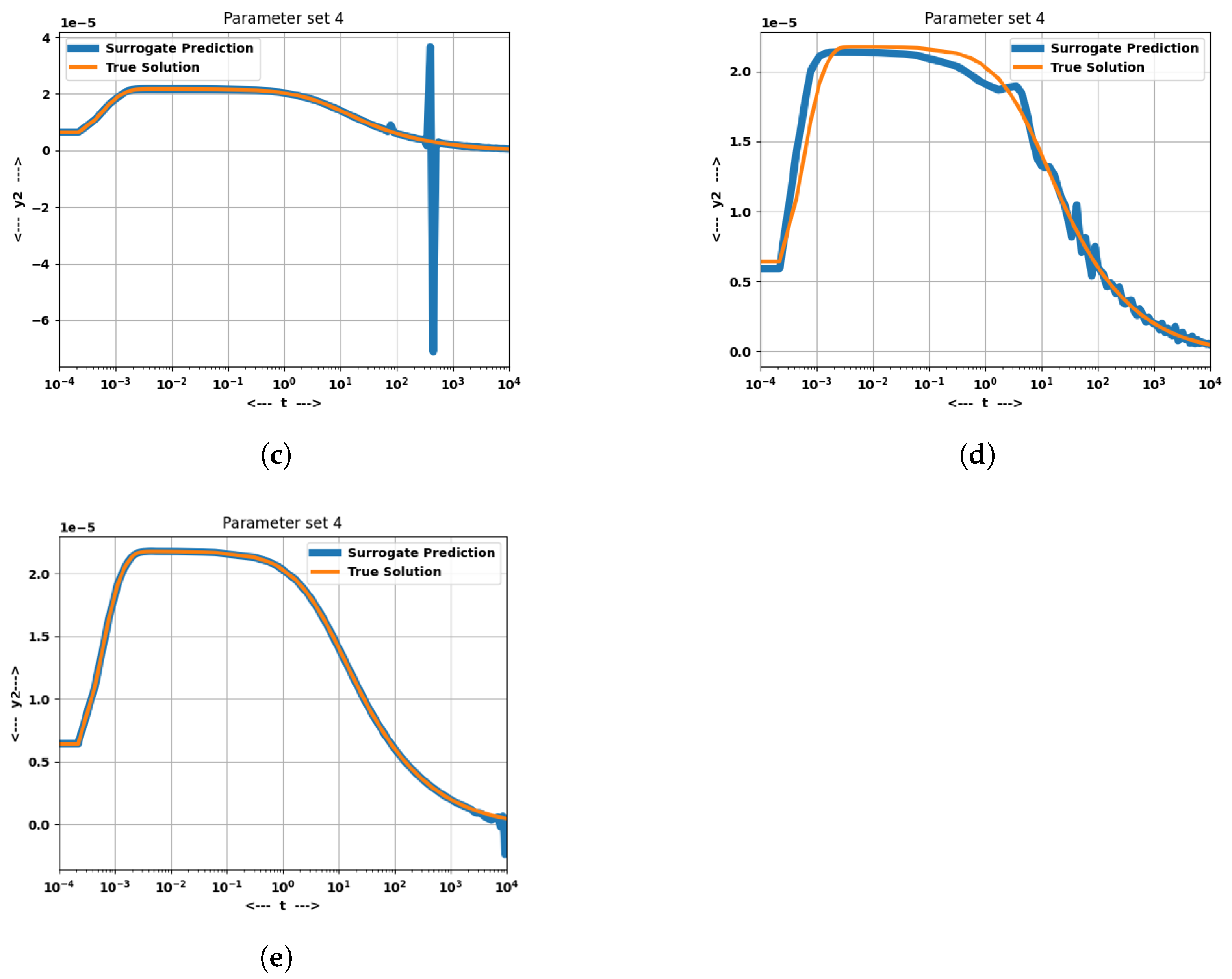
Nonlinear	2.60	2.78	3.01	1.76	2.59

shows the mean absolute errors computed across several test cases (listed in

Table 10. Test parameter values for the POLLU air pollution modeling problem.

Parameter Set	${\mathit{y}}_{2,0}$	${\mathit{y}}_{4,0}$	${\mathit{y}}_{7,0}$
P1	0.192	0.0464	0.114
P2	0.258	0.04012	0.103
P3	0.188	0.0332	0.0938
P4	0.208	0.0508	0.115
P5	0.228	0.0488	0.0714

) for a few species in the reaction, for the linear and nonlinear projection methods. It can be observed that the nonlinear projection CTESN outperforms the linear projection CTESN when all other hyper-parameters are kept the same. Figure 6 shows the comparison of the prediction graphically; the LPCTESN prediction is much noisier than the NLPCTESN prediction at later times. This was also observed with Robertson’s equations, where the predictions at larger time scales by the LPCTESN tended to become noisier.

4. Discussion and Conclusions

From the numerical experiments conducted, it was observed that polynomial-augmented K-Nearest Neighbor RBFs outperform standard RBFs in terms of accuracy when used as part of the CTESN surrogate modeling algorithm. It was observed that the nonlinear projection (NLPCTESN) method consistently outperformed the linear projection (LPCTESN) method, achieving superior accuracy when the hyper-parameters were the same, on a variety of problems. The NLPCTESN method demonstrated accuracy across several problems with sharp transients, varying time scales, and long horizons of integration, whereas the LPCTESN method had a higher generalization error on all test examples. The surrogate was also shown to achieve a speedup of several orders of magnitude compared to an ODE solver of a realistic collision problem and could be used for several cases like design optimization and online collision severity monitoring.

There are several directions in which this work could be built upon. The CTESN is a black-box data-driven method, and future works need to investigate how well the model learns the physics of the problem, or apply physics-constrained modeling approaches to the outputs of the CTESN. The speedup of the surrogate model becomes very apparent when solving many instances of the ODE; this happens either when the ODE system is very large, or the small ODE system has to be solved repeatedly many times, such as in coupled ODE–PDE systems. Examples include chemically reacting flows similar to the POLLU system, in which a large stiff system of ODEs has to be solved at every compute node, or FEM-based crash solvers which require accurate modeling of sharp transients similar to those demonstrated in this work.

References

1. Nascimento, R.G.; Viana, F.A.; Corbetta, M.; Kulkarni, C.S. A framework for Li-ion battery prognosis based on hybrid Bayesian physics-informed neural networks. Sci. Rep. 2023, 13, 13856. [Google Scholar] [CrossRef] [PubMed]
2. Malekloo, A.; Ozer, E.; AlHamaydeh, M.; Girolami, M. Machine learning and structural health monitoring overview with emerging technology and high-dimensional data source highlights. Struct. Health Monit. 2022, 21, 1906–1955. [Google Scholar] [CrossRef]
3. Yousif, M.Z.; Yu, L.; Hoyas, S.; Vinuesa, R.; Lim, H. A deep-learning approach for reconstructing 3D turbulent flows from 2D observation data. Sci. Rep. 2023, 13, 2529. [Google Scholar] [CrossRef] [PubMed]
4. Liu, Y.; Zhao, T.; Ju, W.; Shi, S. Materials discovery and design using machine learning. J. Mater. 2017, 3, 159–177. [Google Scholar] [CrossRef]
5. Liang, J.; Ding, Z.; Han, Q.; Wu, H.; Ji, J. Online learning compensation control of an electro-hydraulic shaking table using Echo State Networks. Eng. Appl. Artif. Intell. 2023, 123, 106274. [Google Scholar] [CrossRef]
6. Li, X.; Bi, F.; Yang, X.; Bi, X. An echo state network with improved topology for time series prediction. IEEE Sensors J. 2022, 22, 5869–5878. [Google Scholar] [CrossRef]
7. Xu, M.; Han, M.; Qiu, T.; Lin, H. Hybrid regularized echo state network for multivariate chaotic time series prediction. IEEE Trans. Cybern. 2018, 49, 2305–2315. [Google Scholar] [CrossRef] [PubMed]
8. Duarte, A.L.; Eisencraft, M. Denoising of discrete-time chaotic signals using echo state networks. Signal Process. 2024, 214, 109252. [Google Scholar] [CrossRef]
9. Ghazijahani, M.S.; Heyder, F.; Schumacher, J.; Cierpka, C. On the benefits and limitations of echo state networks for turbulent flow prediction. Meas. Sci. Technol. 2022, 34, 014002. [Google Scholar] [CrossRef]
10. Gonon, L.; Grigoryeva, L.; Ortega, J.P. Approximation bounds for random neural networks and reservoir systems. Ann. Appl. Probab. 2023, 33, 28–69. [Google Scholar] [CrossRef]
11. Hart, A.; Hook, J.; Dawes, J. Embedding and approximation theorems for echo state networks. Neural Netw. 2020, 128, 234–247. [Google Scholar] [CrossRef]
12. Lambert, J.D. Numerical Methods for Ordinary Differential Systems; Wiley: New York, NY, USA, 1991; Volume 146. [Google Scholar]
13. Ji, W.; Qiu, W.; Shi, Z.; Pan, S.; Deng, S. Stiff-pinn: Physics-informed neural network for stiff chemical kinetics. J. Phys. Chem. A 2021, 125, 8098–8106. [Google Scholar] [CrossRef]
14. Cuomo, S.; Di Cola, V.S.; Giampaolo, F.; Rozza, G.; Raissi, M.; Piccialli, F. Scientific machine learning through physics-informed neural networks: Where we are and what’s next. J. Sci. Comput. 2022, 92, 88. [Google Scholar] [CrossRef]
15. Kim, S.; Ji, W.; Deng, S.; Ma, Y.; Rackauckas, C. Stiff neural ordinary differential equations. Chaos Interdiscip. J. Nonlinear Sci. 2021, 31, 093122. [Google Scholar] [CrossRef]
16. Chen, R.T.; Rubanova, Y.; Bettencourt, J.; Duvenaud, D.K. Neural ordinary differential equations. In Proceedings of the 32nd Conference on Neural Information Processing Systems (NeurIPS 2018), Montréal, QC, Canada, 2–8 December 2018. [Google Scholar]
17. Goswami, S.; Jagtap, A.D.; Babaee, H.; Susi, B.T.; Karniadakis, G.E. Learning stiff chemical kinetics using extended deep neural operators. Comput. Methods Appl. Mech. Eng. 2024, 419, 116674. [Google Scholar] [CrossRef]
18. Lu, L.; Jin, P.; Pang, G.; Zhang, Z.; Karniadakis, G.E. Learning nonlinear operators via DeepONet based on the universal approximation theorem of operators. Nat. Mach. Intell. 2021, 3, 218–229. [Google Scholar] [CrossRef]
19. Gobbert, M.K. Robertson’s Example for Stiff Differential Equations; Technical Report; Arizona State University: Tempe, AZ, USA, 1996. [Google Scholar]
20. Verwer, J.G. Gauss–Seidel iteration for stiff ODEs from chemical kinetics. SIAM J. Sci. Comput. 1994, 15, 1243–1250. [Google Scholar] [CrossRef]
21. Anantharaman, R.; Ma, Y.; Gowda, S.; Laughman, C.; Shah, V.; Edelman, A.; Rackauckas, C. Accelerating simulation of stiff nonlinear systems using continuous-time echo state networks. arXiv 2020, arXiv:2010.04004. [Google Scholar]
22. Roberts, C.; Lara, J.D.; Henriquez-Auba, R.; Bossart, M.; Anantharaman, R.; Rackauckas, C.; Hodge, B.M.; Callaway, D.S. Continuous-time echo state networks for predicting power system dynamics. Electr. Power Syst. Res. 2022, 212, 108562. [Google Scholar] [CrossRef]
23. Anantharaman, R.; Abdelrehim, A.; Jain, A.; Pal, A.; Sharp, D.; Edelman, A.; Rackauckas, C. Stably Accelerating Stiff Quantitative Systems Pharmacology Models: Continuous-Time Echo State Networks as Implicit Machine Learning. IFAC-PapersOnLine 2022, 55, 1–6. [Google Scholar] [CrossRef]
24. Jaeger, H. Echo state network. Scholarpedia 2007, 2, 2330. [Google Scholar] [CrossRef]
25. Viehweg, J.; Worthmann, K.; Mäder, P. Parameterizing echo state networks for multi-step time series prediction. Neurocomputing 2023, 522, 214–228. [Google Scholar] [CrossRef]
26. Lukoševičius, M. A practical guide to applying echo state networks. In Neural Networks: Tricks of the Trade, 2nd ed.; Springer: Berlin/Heidelberg, Germany, 2012; pp. 659–686. [Google Scholar]
27. Rackauckas, C.; Gwozdz, M.; Jain, A.; Ma, Y.; Martinuzzi, F.; Rajput, U.; Saba, E.; Shah, V.B.; Anantharaman, R.; Edelman, A.; et al. Composing modeling and simulation with machine learning in Julia. In Proceedings of the 2022 Annual Modeling and Simulation Conference (ANNSIM), San Diego, CA, USA, 18–20 July 2022; pp. 1–17. [Google Scholar]
28. Horváth, A.; Hatwágner, M.F.; Harmati, I.Á. Searching for a nonlinear ODE model of vehicle crash with genetic optimization. In Proceedings of the 2012 7th IEEE International Symposium on Applied Computational Intelligence and Informatics (SACI), Timisoara, Romania, 24–26 May 2012; pp. 131–136. [Google Scholar]
29. Morris, M.D.; Mitchell, T.J. Exploratory designs for computational experiments. J. Stat. Plan. Inference 1995, 43, 381–402. [Google Scholar] [CrossRef]
30. Cao, D.; Li, X.; Zhu, H. A polynomial-augmented RBF collocation method using fictitious centres for solving the Cahn–Hilliard equation. Eng. Anal. Bound. Elem. 2022, 137, 41–55. [Google Scholar] [CrossRef]
31. Jankowska, M.A.; Karageorghis, A.; Chen, C.S. Improved Kansa RBF method for the solution of nonlinear boundary value problems. Eng. Anal. Bound. Elem. 2018, 87, 173–183. [Google Scholar] [CrossRef]
32. Yao, G.; Chen, C.S.; Zheng, H. A modified method of approximate particular solutions for solving linear and nonlinear PDEs. Numer. Methods Partial Differ. Equ. 2017, 33, 1839–1858. [Google Scholar] [CrossRef]
Figure 1. Depiction of a standard Echo State Network.
Mca 29 00009 g001
Figure 2. Figures show the time history for y 2 for a test parameter set (P2 from Table 1). Each trial mentioned below is referenced from Table 2. The NLPCTESN prediction is the best out of all models. (a) Trial 1 (b) Trial 2 (c) Trial 3 (d) Trial 4 (e) Trial 5.
Mca 29 00009 g002
Figure 3. Figures show time history for y 2 for a test parameter set (P4 from Table 4). Each trial mentioned below is referenced from Table 3. The NLPCTESN performs the best out of all models. (a) Trial 1 (b) Trial 2 (c) Trial 3 (d) Trial 4 (e) Trial 5.
Mca 29 00009 g003aMca 29 00009 g003b
Figure 4. Sliding Basepoint system for collision modeling.
Mca 29 00009 g004
Figure 5. Solution v 2 for several tests with different test parameters, the average error of which is shown in Table 7. The left and right columns show results from the linear and nonlinear projections, respectively. Table 6 defines the values P3–P5 mentioned below. (a) LPCTESN—P3 (b) NLPCTESN—P3 (c) LPCTESN—P4 (d) NLPCTESN—P4 (e) LPCTESN—P5 (f) NLPCTESN—P5.
Mca 29 00009 g005
Figure 6. Solutions y 1 , y 2 , y 14 , and y 20 for a test parameter (P2 from Table 10). The left and right columns contain results from the linear and nonlinear projections, respectively. The NLPCTESN outperforms the LPCTESN in this example. (a) LPCTESN— y 1 (b) NLPCTESN— y 1 (c) LPCTESN— y 2 (d) NLPCTESN— y 2 (e) LPCTESN— y 14 (f) NLPCTESN— y 14 (g) LPCTESN— y 20 (h) NLPCTESN— y 20 .
Mca 29 00009 g006aMca 29 00009 g006b