A Robust FOPD Controller That Allows Faster Detection of Defects for Touch Panels ^†

Abstract

This study aims to synthesize and implement a robust fractional order PD (RFOPD) controller to increase the speed at which defects in automated touch panel inspection systems (ATPISs) are detected. A three-dimensional orthogonal stage (TDOS) driven by BLDC servo motors moves the inspection pen (IP) vertically and horizontally. The dynamic equation relating the BLDC servo motor input to the tip motion is established. A touch position identification (TPI) system is used to locate the touch point rapidly. An RFOPD controller is used to actuate the BLDC servo motors and move the TDOS rapidly and accurately in three dimensions. This method displaces the IP to any specified position and shows user-defined inspection trajectories on the touch screens. The gain-phase margin tester (GPMT) and stability equation methods are exploited to schedule the RFOPD controller gain settings and to maintain the specific safety margins for the controlled system. The simulation studies show that the proposed RFOPD controller exhibits better tracking and disturbance rejection responses than a conventional PID controller. The robustness of the RFOPD-controlled ATPIS, considering unmodeled uncertainties and friction-induced disturbances, is verified through simulation and experimental studies. Several user-defined inspection patterns are used to verify performance, and the experimental results show that the proposed RFOPD controller is effective.

1. Introduction

Touch panels (TPs) are used as an interface for information interactions. They are increasingly used in general industrial and personal applications, such as smartphones, ATMs, sale devices, interface products, industrial control systems, medical instrumentations, and transportation systems. They provide a comfortable, intuitive, and user-friendly touch-based interface for information exchange and are easily used by individuals of all ages. They feature an anti-scratch surface, fast response, and resistance to stains and water.

Defects in touch sensors must be detected early in the production process. The number of smart devices with a touch user interface has significantly increased, and there is increased demand for TPs. ATPISs are used with robotic equipment to emulate various touch commands onto TPs to allow automatic tests of TPs that do not require human intervention.

To manufacture ATPISs, numerous studies propose automated inspection methods to detect defects in TPs [1,2,3,4,5]. Chen et al. [1] used an electronic control system, a mechanism, and machine vision to construct an automated optical inspection method to test defects of resistive TPs. The study used edge detection, Fourier transform, morphology, thresholding, and particle analysis methods to detect and classify defects. Lin and Tsai [2] inspected surface defects in capacitive TPs using the Fourier transform approach. At the center spectrum, they derived four principal high-energy frequency bands. Then, they used a filter to segment these frequency bands to locate defects. For capacitive TPs, Chiang et al. [3] used Fourier transformation to transfer the surface images of TPs and used a band-pass filter to remove ordinary structures. Morphology, binarization, and Canny edge detection methods were then used to recognize defects. Ye et al. [4] used parallel computing techniques to develop a high-resolution AOI system for the fast inspection of defects. The study used a central computer with a graphical processing unit to process images and a back propagation neural network to classify defects. Li et al. [5] proposed an algorithm to search for microfracture defects, broken circuits, and short circuits by determining local connectivity. The study used morphological and fast circuit calculation to detect and classify circuit defects. The developed system detects and distinguishes various defects in TPs quickly and accurately.

Several studies involve robot-assisted inspection of TPs [6,7,8,9,10,11,12]. Jenkinson [6] used a touchscreen testing platform with a robotic tester and an electronic control system for repeatable testing of TPs. This platform uses various conductive tips to simulate human behavior and engage the touch screen. Verma et al. [7] designed a Cartesian robot to operate on touch devices and used the Android debugging bridge to capture different types of touch, such as multiple taps, pinching, single taps, and swiping. This system tests APPs with various orders of action. Wilson et al. [8] proposed a robotic arm that simulates various touch commands for functional tests of TPs. This robotic arm consists of a stylus that moves in three dimensions. Lu and Juang [9] used a five-DOF robot arm to input words onto the TPs for smartphones using the Fuzzy theory to position the robot arm rapidly. Frister et al. [10] proposed several methods to test mobile applications using robotic arms. The proposed system executes black-box tests using a tree-search algorithm. IAI America, Inc. [11] launched a touchscreen tablet that touches the touchscreen with a pen and computes the deviation between the touch and reaction positions. Using this tablet, one operator can inspect twice as many units, so personnel costs are halved. To meet the demand for rapid and nondestructive detection, a PID-like fuzzy controller is proposed in [12] to increase the accuracy and speed of automatic inspection for resistive TPs.

To achieve faster detection of defects for TPs, a homemade ATPIS, involving a TPI system, a three-dimensional inspection pen control (TDIPC) system, and a graphical user interface of the control software (GUICS), is implemented in this study. The TPI system is designed and realized to rapidly locate the touch points on the surface of the TPs. The GUICS is a dashboard that decides the inspection patterns, computes the inspection time, displays the detected touch points, and determines whether the inspection is a pass or a fail. The kernel part of the TDIPC is a TDOS, which includes a vertical translation Z-stage and a ball-screw-driven X-Y (BSDXY) stage. It actuates the IP to move vertically and horizontally. The BSDXY stage comprises two orthogonal single-axis ball-screw-driven (SABSD) stages that are actuated independently along the X- and Y-axis directions using two BLDC servo motors. A compact linear actuator drives the vertical translation stage in the Z direction. To accomplish rapid and precise control of the TDOS, the transfer function that relates the BLDC servo motor input to the horizontal position of the IP is deduced.

Many different control strategies have been proposed to achieve rapid and accurate output tracking for a specific class of control systems [13,14,15]. Fractional control attracts theoretical and practical interest in the control field [16]. Based on these results, in this study, an RFOPD controller, retaining two more adjustable parameters than classical PID controllers, is used to increase robustness, enhance tracking responses, and reduce excess overshoot of the homemade ATPIS. The RFOPD controller drives the TDOS, allowing the IP to track any pre-defined inspection trajectory rapidly and accurately and thus, increasing the speed with which capacitive or resistive TPs are inspected.

Different fractional-order PID controller tuning methods are found in [17,18,19,20,21,22,23]. The GPMT method [24,25,26], accompanied by the stability equation method [27], is used to tune the RFOPD controller to ensure the controlled system maintains the designer-specified robust margins. Prior to applying this method, the designer does not need to reduce the order of the model or approximate any possible process delay terms. A feasible specifications-oriented region (FSOR) enclosing all feasible FOPD controller gains can be located in the K_P–K_D parameter plane. The FOPD controllers encompassed by the FSOR are non-conservative and reliable, ensuring stability and maintaining the pre-specified GM and PM. Instead of just one, a set of viable FOPD gain sets is available for selection, thereby significantly enhancing the flexibility in choosing controller coefficients. This flexibility facilitates considering potential uncertainties encountered in implementing this FOPD controller. An RFOPD controller candidate is selected from this FSOR based on a given IAE criterion, thus permitting a satisfactory tracking response. As a result, the proposed method ensures both robustness and performance.

Matlab-based simulation studies are used to compare the performance of the proposed RFOPD controller with that of a conventional PID controller. The simulation studies show that the proposed RFOPD controller allows better tracking and disturbance rejection responses than a traditional PID controller. Diagonal-line, rectangular-type, circular-type, convergent-type, round-type, and rhombus-type inspections are conducted to verify the proposed RFOPD controller experimentally. The ATPIS with this controller allows rapid and accurate inspections while maintaining robustness in the face of modeling uncertainties and friction-induced disturbances.

2. Automated Touch Panel Inspection System

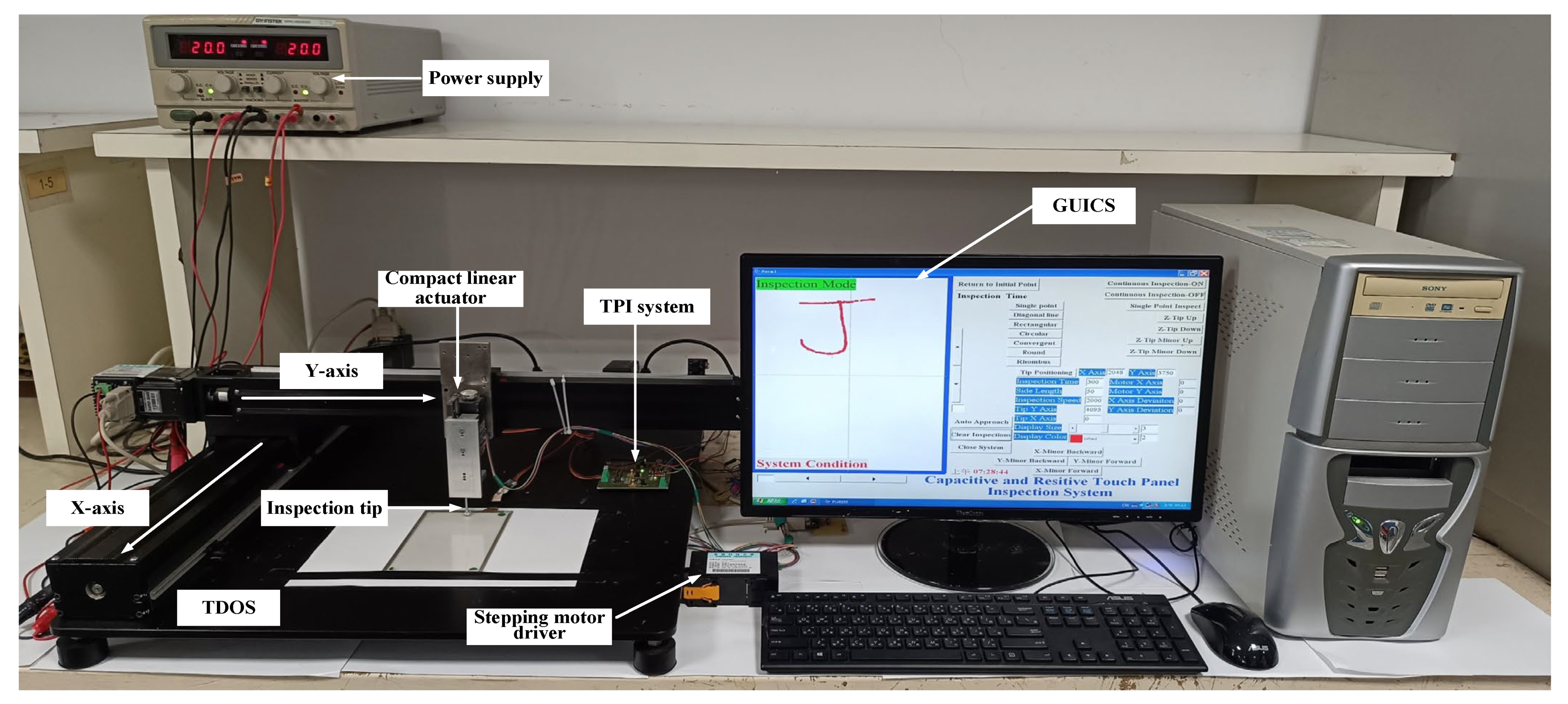
Figure 1 shows a photograph of the homemade ATPIS. It is an electromechanical system with three main subsystems: the TPI system, the three-dimensional inspection pen control (TDIPC) system, and the graphical user interface of the control software (GUICS). The individual purposes are detailed below.

2.1. Touch Position Identification System

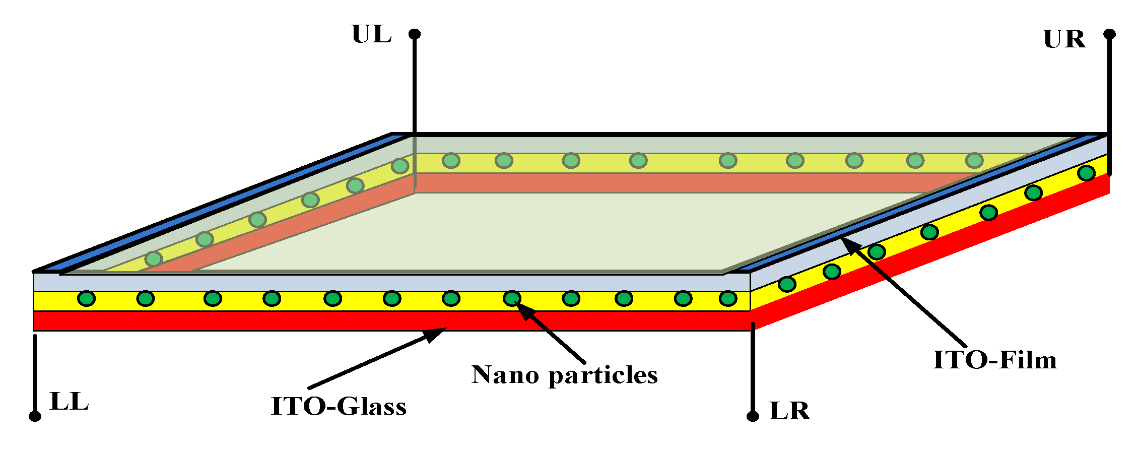
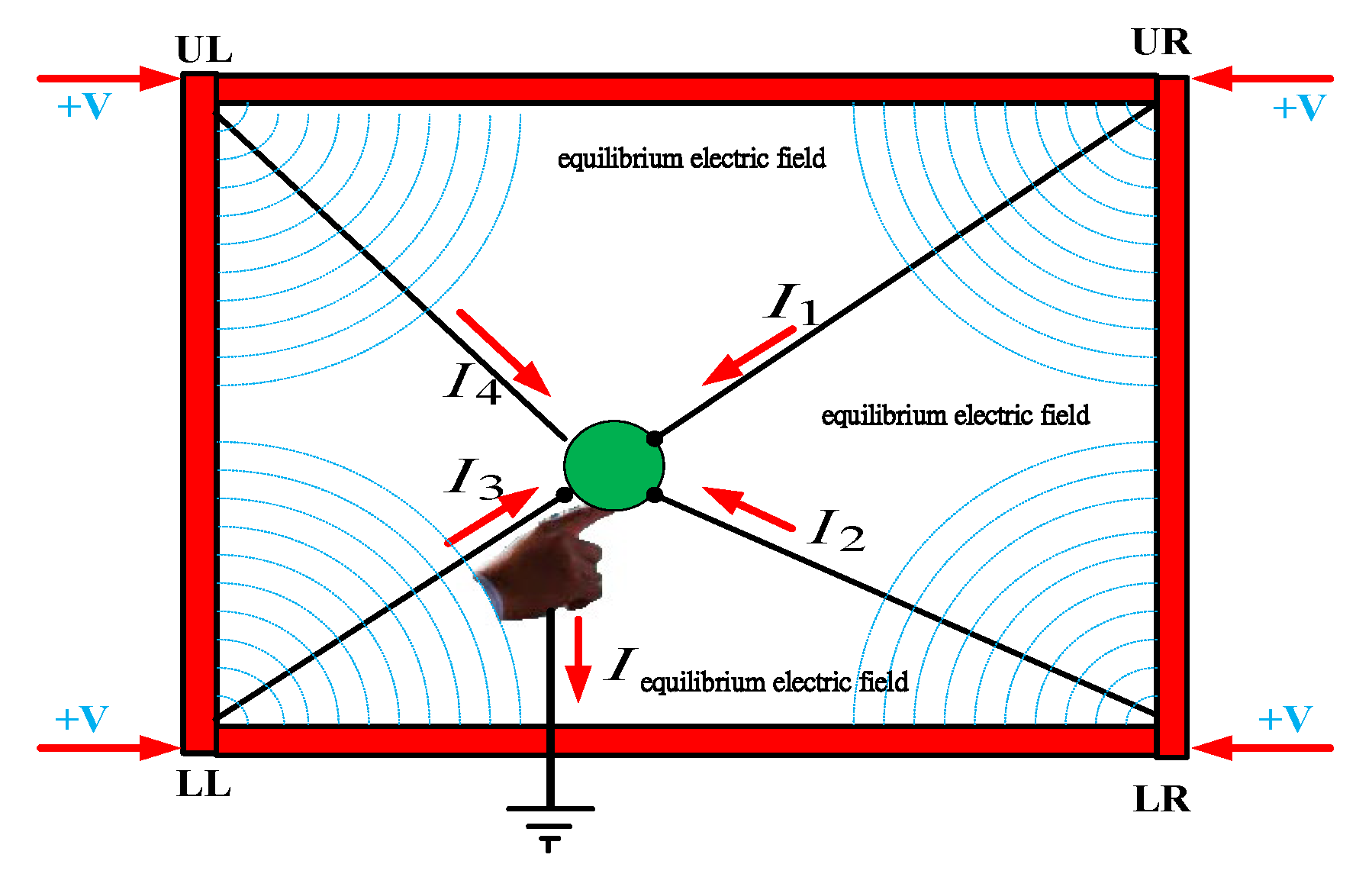
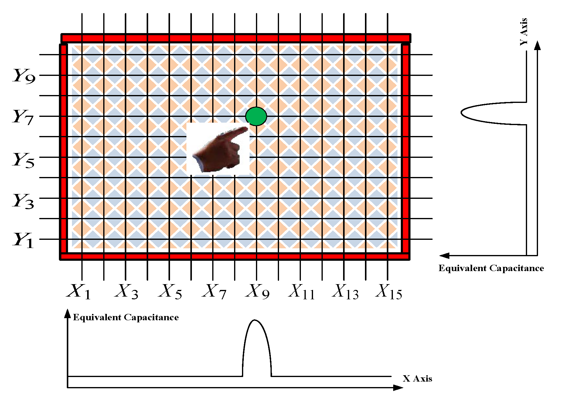
Resistive four- and five-wire touch systems and capacitive touch screens are the most common technologies currently available. Due to their longevity, resistive TPs are widely used in industrial products, ATMs, kiosks, and medical equipment. Capacitive TPs are responsive, efficient, and adaptable and have overtaken resistive TPs as the dominant touch-sensing technology for cell phones and tablet computers. Figure 2, Figure 3 and Figure 4 show the internal structure of resistive and capacitive TPs.

The TPI subsystem immediately detects variations in the resistance or capacitance of the TP surface. It converts these variations in physical properties at the touch point into voltage signals, which are used to calculate the coordinates of the touch points. This TPI system continuously and rapidly identifies the touch points and transmits their coordinates to the GUICS.

2.2. Three-Dimensional Inspection Pen Control System

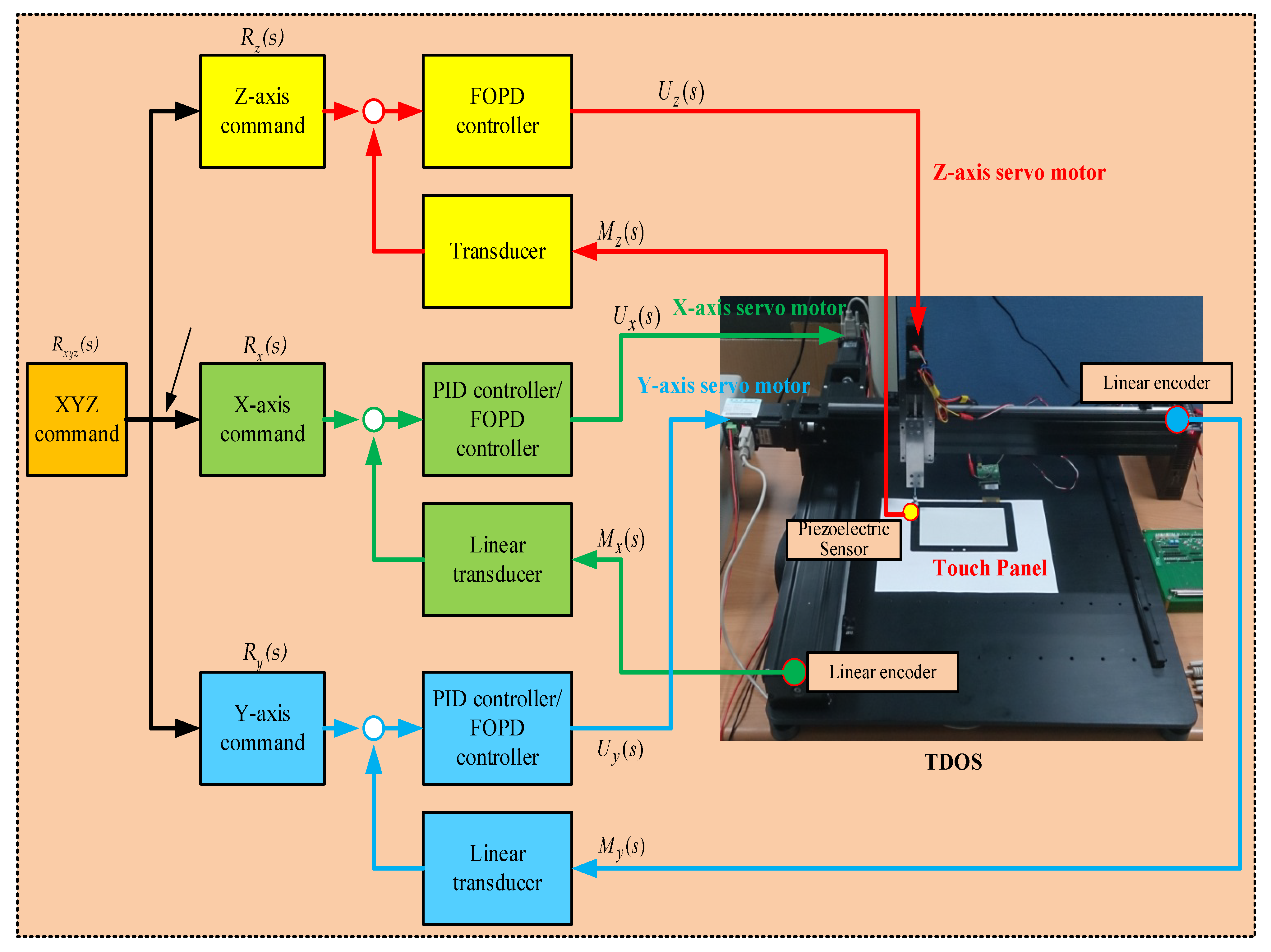
Figure 5 shows a photograph and the associated signal flow diagram of the TDIPC system. The TDIPC system involves a TDOS mechanism and three PID/FOPD controllers. The PID/FOPD controllers are realized inside the GUICS. The TDOS is the essential part of the TDIPC system and contains a horizontal motorized BSDXY stage and a vertical translation Z-stage.

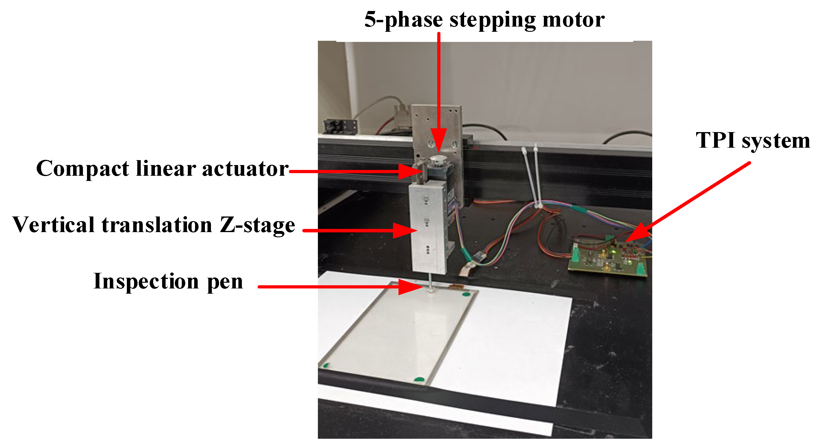
In the vertical direction, Figure 6 shows that the IP is mounted at the lower end of the Z-stage. A compact linear actuator with a five-phase stepping motor drives the Z-stage and moves the IP along the Z-axis. The travel range for the Z-stage is 20 mm. It achieves highly accurate positioning using a space-saving design. A piezoelectric sensor attached to the tip of the IP is used to detect the interaction force between the IP and the touch panel. A transducer then converts the output signal from the piezoelectric sensor into a voltage signal. A digital PID controller is realized as a software algorithm inside the GUICS. This controller receives the voltage signal from the transducer and maintains a constant interaction force between the IP and the touch panel during testing. The motion along the Z-axis is designed to move at a speed faster than the motion of the BSDXY stage, so the Z-axis dynamic for the TDOS is ignored for this study.

In the horizontal direction, the X- and Y-axis of the BSDXY stage are independent and perpendicular to each other. Heuristically, the simultaneous movement of these two axes displaces the IP to any surface point on the panel under inspection. A linear SABSD stage with a BLDC servo motor achieves motion along each axis. Linear encoders and transducers convert the position of the moving table of the SABSD into digital signals.

In recent years, SABSD systems have replaced lead screw systems because they allow for accurate positioning and offer low cost, reliability, repeatability, generality, high load capacity, long fatigue life, and high efficiency in almost every application [28,29,30]. They are widely used in most numerically controlled high-speed machine tools for material handling, testing, inspection, and manufacturing. They are also very rigid and feature a very low coefficient of friction, so there is sufficient force when the rotational movement of the BLDC servo motors is converted into a linear motion for the moving tables.

2.3. The Graphical User Interface of the Control Software

Figure 7 shows the control panel of the GUICS for the ATPIS. The right part of the GUICS is the command region. The left part of the GUICS, outlined in blue and identified as the white rectangle area, is the touch coordinate display region (TCDR). This region shows the coordinates of any touch event immediately. The GUICS application is developed using a visual component-based object-oriented framework in the environment of C++ Builder 10.0 on Microsoft Windows 10. Before testing TPs, the control buttons, “Z-Tip Up”, “Z-Tip Down”, “Z-Tip Minor Up”, and “Z-Tip Minor Down”, are used to move the inspection tip up or down rapidly or slowly. The “Auto Approach” button automatically moves the inspection pen to contact with the touch panel. The GUICS uses the control buttons, “X-Minor Backward”, “X-Minor Forward”, “Y-Minor Backward”, and “Y-Minor Forward”, to drive the BSDXY stage and move the inspection pen laterally.

During inspections, the GUICS moves the IP to the specified position using the BSDXY stage. The GUICS also determines the coordinates of the touch points from the TPI system and displays them immediately in the TCDR. It compares the touch and the detected coordinates for the IP and determines whether the inspection is a pass or a fail. It performs single-point, diagonal-line, rectangular-type, circular-type, convergent-type, round-type, and rhombus-type inspections and shows the total inspection time. In addition to linearity tests, this GUICS conducts reliability and touch pressure tests.

A mathematical model that describes the motion of the BSDXY stage is used to move the IP to the specified position rapidly and accurately. The mathematical model for the BSDXY stage is described in terms of its physical, mechanical, and dynamical parameters.

3. Modeling the Ball-Screw-Driven X-Y Stage

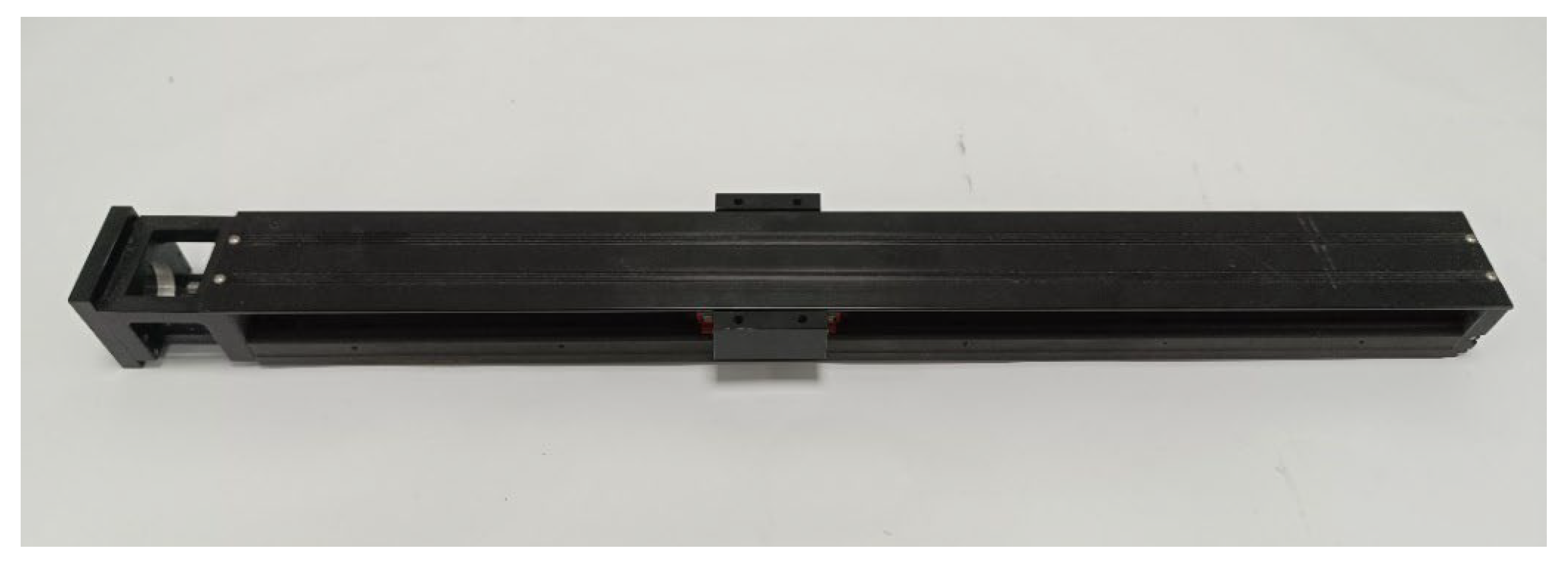
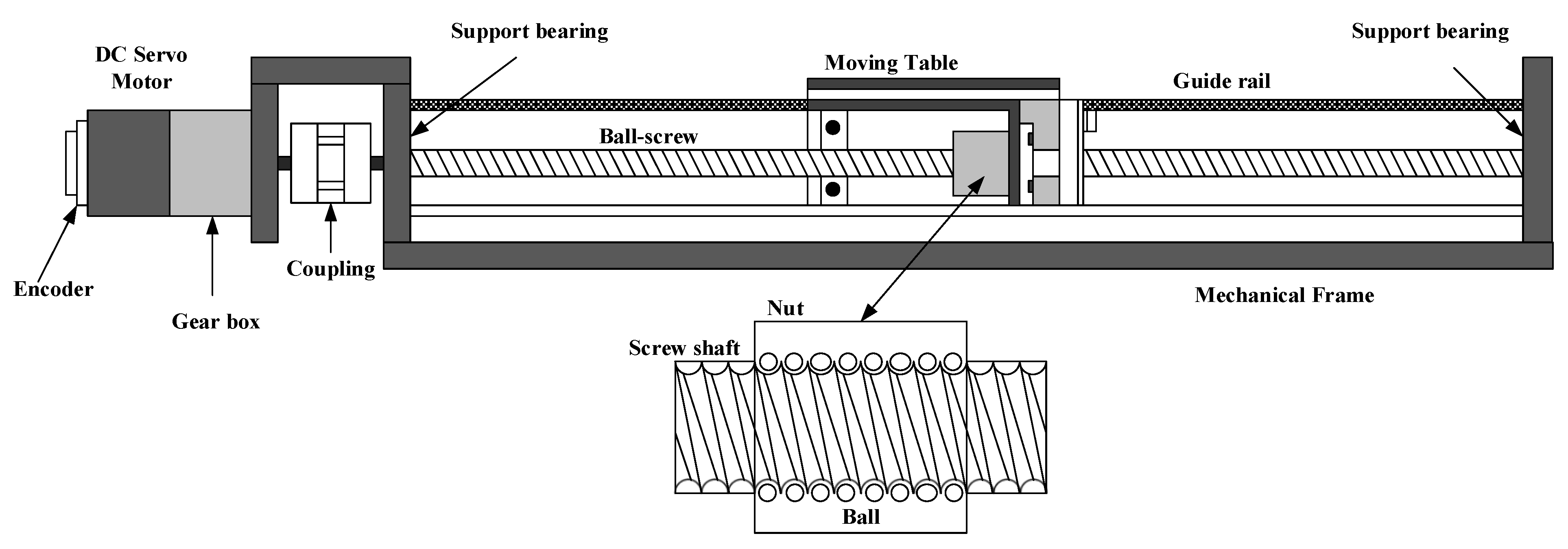
The BSDXY stage uses two independent SABSD stages driven by separate BLDC servo motors. A servo driver controls each BLDC motor. The control structure for the BSDXY stage, which uses two BLDC servo motors, comprises two independent SISO position control systems. The mechanism for the X-stage is similar to that for the Y-stage. The maximum travel range for the X-stage and the Y-stage is 600 mm. A linear encoder with a resolution of 0.5 mm/pulse is used to measure the movement of the SABSD stages. The Y-stage is fixed on the moving table of the X-stage, so the X-stage is heavier (total mass 9.4 kg) than the Y-stage. The Y-stage only supports the mass of the Z-stage and the moving table and weighs about 4.2 kg. Figure 8 shows an electro-mechanical photograph of the SABSD stage. Figure 9 shows a schematic diagram of the SABSD stage. The SABSD stage control system comprises four central units: the electronics control unit, the BLDC servo motor, the ball-screw-driven stage, and the signal detection unit.

The electronics control unit drives the BLDC servo motor to rotate and generates torque transmitted to the connected ball-screw. Using a signal detection device, this unit also measures the motor’s dynamics and the moving table’s displacement. These measured signals are fed into the PID/FOPD controllers to generate the optimal control efforts to schedule the driving signals for the BLDC servo motors.

The motor for this study is a 150W/SLIM7-3903 BLDC servo motor, manufactured by the CSIM Inc. from New Taipei City of Taiwan, coupled to a rotational 2000 PPR encoder. This encoder is an electric component that transduces the detected voltage signal into a torque and an angular shaft displacement. The motor has a maximum speed of 3000 rpm, a nominal torque of 0.477 Nm, and a maximum torque of 1.432 Nm. This motor drives the moving table through a gearbox, a coupling, a ball-screw, and a nut-screw transmission mechanism.

The SABSD stage is rigidly connected to the BLDC servo motor via a coupling. This is a precision linear component with a ball-screw and composes a moving table, a mechanical frame, a nut, a screw shaft, guide rails, and support bearings. There are small steel balls between the screw and the nut to prevent the two bodies from touching and significantly reduce friction and the generation of heat. Using a ball-screw, this stage converts the motor’s rotation into a linear movement for the moving table. The linear travel range for each complete turn of this ball-screw is 10 mm. As shown in Figure 9, the displacement of the moving table is determined using the kinematic relationship between the BLDC servo motor and the SABSD stage.

The signal detection unit detects the displacement of the moving table using a linear encoder with a linear resolution of 250 nm. This unit also characterizes the dynamics of the BLDC servo motors via the rotational encoder.

To achieve rapid and accurate control of this SABSD stage, an equation is derived to describe the motion of the SABSD stage.

Modeling of the Single-Axis Ball-Screw-Driven Stage

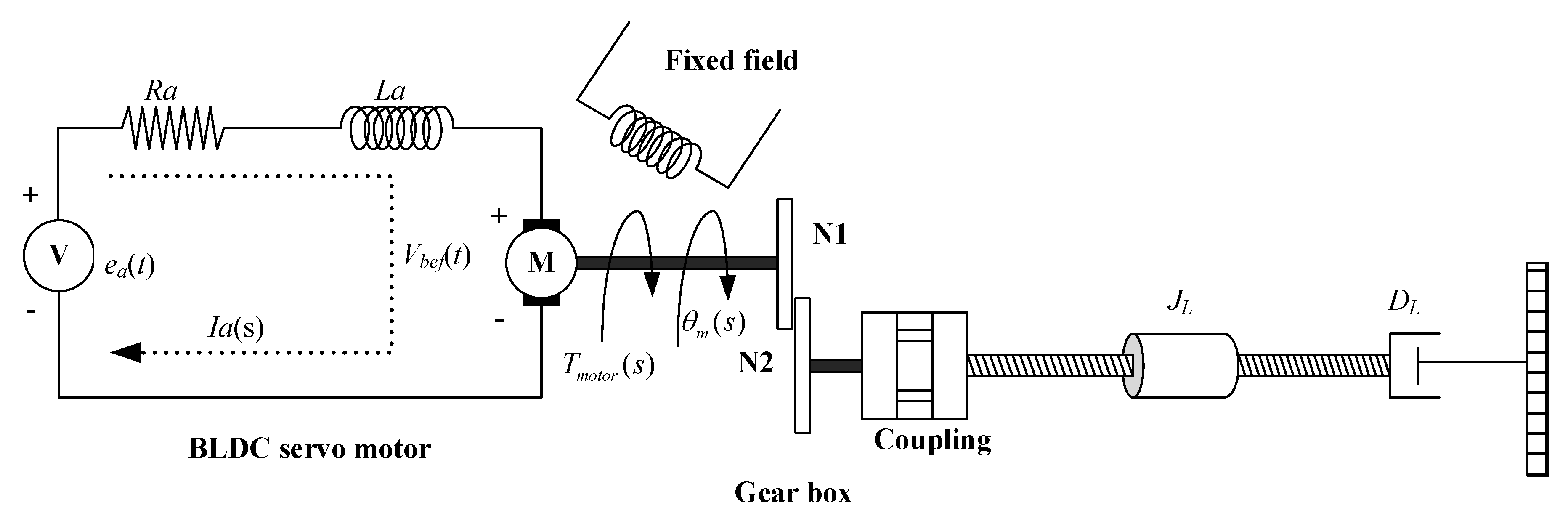
The modeling of the SABSD stage involves two stages. The transfer function from the BLDC servo motor’s applied voltage to the rotor’s angular position is determined. Then, the transfer function relating the rotor’s angular position to the linear position of the moving stage is determined. Figure 10 shows a schematic diagram of an SABSD stage driven by a BLDC servo motor.

Figure 10 shows that a stationary permanent magnet generates a fixed magnetic field. A rotating armature circuit passes through this fixed field and generates a force that turns the motor’s rotor and activates the motor to rotate. This force is defined as

$$F=Bl{i}_a(t),$$

(1)

where i_a(t), B, and l are, respectively, the armature current, the magnetic field intensity, and the conductor length.

As the motor starts to rotate, a back electromotive force (back emf) is generated at the conductor terminals. This back emf, which is proportional to the rotational speed of the current-carrying armature, is expressed as

$$V_{bef}(t)=K_{bef}\frac{\mathrm{d}{\theta }_m(t)}{\mathrm{d}t},$$

(2)

where K_bef is the back emf constant and θ_m(t) is the angular advance of the motor.

Equation (2) undergoes a Laplace transformation to become

$$V_{bef}(s)=K_{bef}s{\theta }_m(s).$$

(3)

For Figure 10, a loop equation that describes the relationship between the armature current, the back emf, and the applied armature voltage is written as

RI_a(s) + LsI_a(s) + V(s) = E(s),

(4)

where E(s) denotes the Laplace transform of e(t).

The loop current I_a(s) is proportional to the torque T_motor(s) for the motor, so the equation that describes the relationship between the torque and the armature current is written as

T_motor(s) = K_T I_a(s),

(5)

where K_T denotes the torque constant for the motor.

This torque is used to drive the motor that is connected to the ball-screw through a gearbox and a coupling, so

$$T_{motor}(s)=J_m{s}^2{\theta }_m(s)+D_{m}s{\theta }_m(s),$$

(6)

where

$$J_m=J_a+{\left(\frac{N_1}{N_2}\right)}^2{J}_L,$$

(7)

and

$$D_m=D_a+{\left(\frac{N_1}{N_2}\right)}^2{D}_L,$$

(8)

are, respectively, the equivalent inertia and viscous damping at the armature. The motor has the viscous damping D_a and inertia J_a at the armature. The load has the equivalent viscous damping D_L and inertia J_L. D_L and J_L are reflected back to the armature through the gearbox in the ratio (N₁/N₂).

The equivalent load inertia J_L for the SABSD stage is calculated as

$$J_L=J_C+J_{BS}+J_{MS},$$

(9)

where J_C, J_BS, and J_MS are the inertia of the shaft coupling, the ball-screw, and the moving stage, respectively.

The value for J_C is specified in the product manual. The inertia of a ball-screw with a cylindrical structure is written as

$$J_{BS}=\gamma L_{BS}\frac{\pi {D_{BS}}^4}{32},$$

(10)

where γ, L_BS, and D_BS are, respectively, the density, length, and diameter.

The inertia of the moving stage is written as

$$J_{MS}=M_{MS}{\left(\frac{P}{2\pi }\right)}^2,$$

(11)

where M_MS denotes the mass of the moving stage, and P is the pitch length.

For ease of analysis, assume that the axial damping of the ball-screw, the viscous friction of the moving stage, the structural damping of the coupling, and the rotational damping of the gearbox are ignored. Accordingly, the equivalent load damping for the SABSD stage, D_L, is calculated as

$$D_L=D_t+D_{screw}+D_{sn},$$

(12)

where D_t, D_screw, and D_sn are the axial damping of the table, the screw, and the axial damping of the ball-screw and nut transmission, respectively.

Using Equations (4)–(12), the transfer function relating the applied armature voltage and the rotation dynamics of the motor is

$$\frac{{\theta }_m(s)}{E_a(s)}=\frac{K_T}{\left(R_a+L_{a}s\right)\left(J_m{s}^2+D_{m}s\right)+K_{bef}{K}_{T}s}.$$

(13)

Figure 9 shows that a mechanical coupling element is attached to an end of the motor rotor with a gearbox and to the ball-screw shaft. These mechanical elements transform the angular displacement of the BLDC servo motor into linear movement for the moving stage.

Assume that the rolling friction in the ball-screw assembly with normal lubrication is tiny and its influence can be ignored. Consequently, the nut travels on the rotating ball-screw shaft with minimal friction, allowing the ball-screw to support heavy axial loads. Due to the SABSD system’s high rigidity, the clearance might be diminished. Furthermore, as the ATPIS has lower precision requirements, the minor clearance is assumed to have negligible effects on positioning responses and is treated as zero.

The ball-screw attached to a moving stage is kinematically coupled to the motion of the motor. The kinematics of the moving stage are related to the kinematics of the ball-screw by a transformation ratio:

$$r_R^T=\frac{P}{2\pi }.$$

(14)

The dynamic relationship between the rotational motor and the moving stage is described as

$$X(s)=r_R^T\theta (s),$$

(15)

which characterizes the dynamics of the moving stage.

Using Equations (13)–(15), the governing equation for the SABSD stage that relates the applied voltage for the BLDC servo motor to the position of the moving stage is described as

$$\frac{X(s)}{E_a(s)}=\frac{r_R^T{K}_T}{\left(R_a+L_{a}s\right)\left(\left(J_m{s}^2+D_{m}s\right)\right)+K_{bef}{K}_{T}s}$$

(16)

The main system parameters used to formulate the SABSD stage are listed in

Table 1. Parameters for the SABSD stage.

Parameter	Description	Quantity
Kbef	back emf constant	0.03525 V/(rad/s)
KT	torque constant of the motor	0.03525 Nm/A
Ra	motor’s resistance	0.248 Ω
La	motor’s inductance	0.389 mH
N	gear ratio	5
$r_R^T$	transformation ratio	0.01/2π m/rev
Da	equivalent viscous damping of the motor	2.5 × 10−3 Nms/rad
Ja	equivalent inertia of the motor	0.02998 kg·m2
γ	density of the ball-screw	7.9 × 103 kg/m3
LBS	ball-screw length	0.6 m
DBS	ball-screw diameter	0.012 m
$P$	pitch length of the ball-screw	0.01 m
MMS	mass of the moving stage	0.5 kg
JMS	inertia of the moving stage	1.27 × 10−6 kg·m2
JBS	inertia of the ball-screw	9.6495 × 10−6 kg·m2
JC	inertia of the shaft coupling	2.0255 × 10−6 kg·m2
Dt	axial damping of the table	0.15 × 10−2 Nm/s
Dscrew	axial damping of the screw	2.5 × 10−2 Nm/s
Dsn	axial damping of the ball-screw and nut transmission	2.5 × 10−2 Nm/s

. These parameters are determined from the mechanical components’ experimental system or data sheets. Substituting the values for the parameters in Table 1 into Equation (16) gives

$$\frac{X(s)}{E_a(s)}=\frac{0.5613}{0.1166s^3+74.37s^2+23.73s}$$

(17)

The SABSD systems for the X-stage and Y-stage have the same mechanical structure, driven by BLDC servo motors of the same model, but operate under different load conditions. Consequently, the governing equation for the Y-stage is similar to that of the X-stage.

4. Design for a Robust FOPD Controller for the BSDXY Stage

To allow faster inspection and significantly reduce the test time for each TP item, the ATPIS system must move the IP to a specified position or follow a pre-defined inspection trajectory swiftly and precisely so the X-stage and the Y-stage must be controlled such that the BSDXY stage displaces to any pre-specified point accurately and rapidly. External disturbances, unmodeled dynamics, and parametric uncertainties have a negative effect on the accurate control of the SABSD stage [31]. External disturbances include the load friction that acts on the moving table, the rolling friction in the ball-screw inverter, and the friction between the rotor, the coupling, and the screw shaft. There are also unmodeled dynamics in the electrical and mechanical subsystems. These are the most significant factors affecting the BSDXY stage’s positioning responses.

Because of these uncertainties and disturbances, traditional PID controllers are used for ATPISs. This study accelerates the tracking responses and compensates for these factors and uncertainties using a novel robust FOPD controller, which is written as

$$C_{FOPD}(s)=K_P+K_D\frac{s^{\mu }}{{\tau }_{f}s+1}$$

(18)

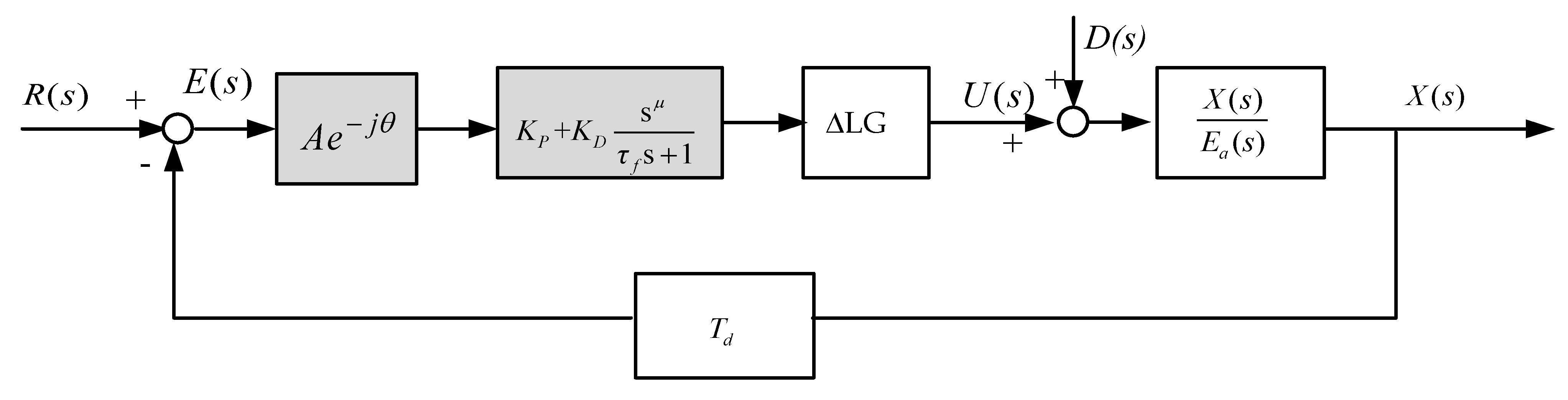
This controller allows rapid trajectory tracking and accurate arrival at a specified position. K_P and K_D represent the proportional and differentiation parameters, respectively, τ_f denotes the filter factor for the differentiation operator, and μ is the non-integer order of the derivative term. μ represents any positive real number within the interval [0, 2]. Figure 11 shows a simplified block diagram for the FOPD-controlled SABSD system with a GMPT [24,25,26], where R(s) and X(s) denote the specified and detected touch point position, respectively, D(s) represents the external disturbances that chiefly involve the load force and friction, U(s) means the controller output, and T_d denotes the sum of the transport and computation times. ΔLG denotes the possible loop gain (LG) variations. The GMPT, $A{e}^{-j\theta }$, guarantees the gain margin (GM), A, and phase margin (PM), θ, for the closed-loop controlled system.

4.1. Tuning of the RFOPD Controller

To tune the gains for the RFOPD controller, all the blocks in Figure 11 and the results in [24,25,26] are used to derive an equation that characterizes the stability conditions for the SABSD system as

$${\zeta }_{FOPD}(s,A,\theta ,T_d,K_P,K_D,\mu )=1+A{e}^{-j\theta }\cdot \left(K_P+K_D\frac{s^{\mu }}{{\tau }_{f}s+1}\right)\cdot \left(\frac{0.056}{0.012s^3+7.437s^2+2.373s}\right)e^{-s{T}_d}=0,$$

(19)

which is further re-written as

$${\zeta }_{FOPD}(s,A,\theta ,T_d,K_P,K_D,\mu )=1+A{e}^{-j\theta }\cdot \left(\frac{\left({\tau }_{f}s+1\right)K_P+K_D{s}^{\mu }}{{\tau }_{f}s+1}\right)\cdot \left(\frac{0.056}{0.012s^3+7.437s^2+2.373s}\right)e^{-s{T}_d}=0.$$

(20)

Multiplying Equation (20) by $\left({\tau }_{f}s+1\right)\cdot \left(0.012s^3+7.437s^2+2.373s\right)$ gives

$$\begin{array}{cc}\hfill {\zeta }_{FOPD}(s,A,\theta ,T_d,K_P,K_D,\mu )=({\tau }_{f}s+1)\cdot (0.012s^3& +7.437s^2+2.373s)+\hfill \\ \hfill \hspace{1em}\hspace{1em}\hspace{1em}\hspace{1em}\hspace{1em}\hspace{1em}\hspace{1em}\hspace{1em}\hspace{1em}\hspace{1em}\hspace{1em}\hspace{1em}\hspace{1em}\hspace{1em}\hspace{1em}\hspace{1em}\hspace{1em}\hspace{1em}\hspace{1em}\hspace{1em}\hspace{1em}& A{e}^{-j\theta }\cdot \left(K_P\left({\tau }_{f}s+1\right)+K_D{s}^{\mu }\right)\cdot \left(0.056\right)\cdot e^{-s{T}_d}=0.\hfill \end{array}$$

(21)

If the frequency for controller design ranges from ${\omega }_{\min }$ to ${\omega }_{\max },$ the interest frequency interval is $\Omega =\left\{\omega \left|{\omega }_{\min }\le \omega \le {\omega }_{\max }\right.\right\}.$ Substituting $s=j\omega$ and $s^{\mu }=p+jr,$ Equation (21) is decomposed into real and imaginary components. Expressing these two components as functions of the controller gains, K_P and K_D, gives

$${\zeta }_{FOPD}^{\mathrm{Re}al}\left(\omega ,A,\theta ,T_d,\mu ,K_P,K_D\right)=B_{FOPD}^1\times K_P+C_{FOPD}^1\times K_D+0.056=0,\forall \omega \in \Omega ,$$

(22)

$${\zeta }_{FOPD}^{\mathrm{Im}ag}\left(\omega ,A,\theta ,T_d,\mu ,K_P,K_D\right)=B_{FOPD}^2\times K_P+C_{FOPD}^2\times K_D+0.056\omega {\tau }_f=0,\forall \omega \in \Omega ,$$

(23)

where

$$B_{FOPD}^1=\left(-7.437{\omega }^2\mathrm{Re}\left(\Psi \right)-\left(0.012{\omega }^3-2.373\omega \right)\mathrm{Im}\left(\Psi \right)\right)-\left(7.437{\omega }^2\mathrm{Im}\left(\Psi \right)-\left(0.012{\omega }^3-2.373\omega \right)\mathrm{Re}\left(\Psi \right)\right)\omega {\tau }_f,$$

(24)

$$C_{FOPD}^1=\left(-7.437{\omega }^2\mathrm{Re}\left(\Psi \right)-\left(0.012{\omega }^3-2.373\omega \right)\mathrm{Im}\left(\Psi \right)\right)p-\left(7.437{\omega }^2\mathrm{Im}\left(\Psi \right)-\left(0.012{\omega }^3-2.373\omega \right)\mathrm{Re}\left(\Psi \right)\right)r,$$

(25)

$$B_{FOPD}^2=\left(-7.437{\omega }^2\mathrm{Re}\left(\Psi \right)-\left(0.012{\omega }^3-2.373\omega \right)\mathrm{Im}\left(\Psi \right)\right)\omega {\tau }_f+\left(7.437{\omega }^2\mathrm{Im}\left(\Psi \right)-\left(0.012{\omega }^3-2.373\omega \right)\mathrm{Re}\left(\Psi \right)\right),$$

(26)

$$C_{FOPD}^2=\left(-7.437{\omega }^2\mathrm{Re}\left(\Psi \right)-\left(0.012{\omega }^3-2.373\omega \right)\mathrm{Im}\left(\Psi \right)\right)r+\left(7.437{\omega }^2\mathrm{Im}\left(\Psi \right)-\left(0.012{\omega }^3-2.373\omega \right)\mathrm{Re}\left(\Psi \right)\right)p,$$

(27)

and

$$\Psi (A,\theta ,T_d,\omega )=A\left[\cos \theta \times \cos \omega T_d-\sin \theta \times \sin \omega T_d\right]-jA\left[\cos \theta \times \sin \omega T_d+\sin \theta \times \cos \omega T_d\right]$$

(28)

Equations (22) and (23) are the stability equations [27]. For $\forall \mu \in \left(0,2\right)$ and $\forall \omega \in \Omega ,$, Cramer’s rule is used to solve Equations (22) and (23) simultaneously for K_P and K_D to give

$$K_P\left(\omega ,A,\theta ,T_d,\mu \right)=\frac{C_{FOPD}^1(·)\times 0.056\omega {\tau }_f-C_{FOPD}^2(·)\times 0.056}{J_1(·)},\forall \mu \in \left(0,2\right),\forall \omega \in \Omega ,$$

(29)

and

$$K_D\left(\omega ,A,\theta ,T_d,\mu \right)=\frac{B_{FOPD}^1(·)\times 0.056\omega {\tau }_f-B_{FOPD}^2(·)\times 0.056}{J_1(·)},\forall \mu \in \left(0,2\right),\forall \omega \in \Omega ,$$

(30)

where

$$J_1\left(\omega ,A,\theta ,T_d,\mu \right)\triangleq \left|\begin{array}{cc}{B}_{FOPD}^1(·)& C_{FOPD}^1(·)\\ B_{FOPD}^2(·)& C_{FOPD}^2(·)\end{array}\right|=B_{FOPD}^1(·)\times C_{FOPD}^2(·)-B_{FOPD}^2(·)\times C_{FOPD}^1(·),\forall \mu \in \left(0,2\right),\forall \omega \in \Omega .$$

(31)

For stability, the specifications are given as GM = 5 dB and PM = 30 degrees. According to the results of [17,18,19], it is found that, for μ > 1.00, the stability region (SR) in the K_P–K_D plane initially expands with an increasing μ. However, with further increments in μ, the SR begins to retract. On the other hand, for μ < 1.00, the SR enlarges as μ decreases. However, with a further decrease in μ, the SR expands to the left and enters the second quadrant of the K_P–K_D plane. Normally, controller gains selected from this quadrant of the K_P–K_D plane tend to generate undesired undershoot phenomena in time response. Based on these results, μ = 1.10 is used in this study to enlarge the SR slightly. This provides us more flexibility in choosing the K_P and K_D gains and increases the relative robustness of the selected controllers.

By letting μ = 1.10 and sweeping the frequency ω from 0.01 to 1000 rad/s, Equations (29)–(30) are used to compute all feasible (K_P, K_D)_{GM=5 dB}, (K_P, K_D)_{PM=30 Deg}, and (K_P, K_D)_{GM=0 dB} solution sets. These three solution sets are plotted on the K_P–K_D plane in Figure 12, illustrating the boundaries for 5 dB, 30 Deg, and the stability boundary. In terms of the results of previous studies [24,25,26,27], the shaded region, FSOR(K_P, K_D), encloses the intersection area of the boundaries for 5 dB and 30 Deg. The FSOR(K_P, K_D) region surrounds all possible RFOPD gain points that satisfy user-specified constraints. This region is mathematically expressed as S_FOPD(K_P, K_D, μ = 1.10).

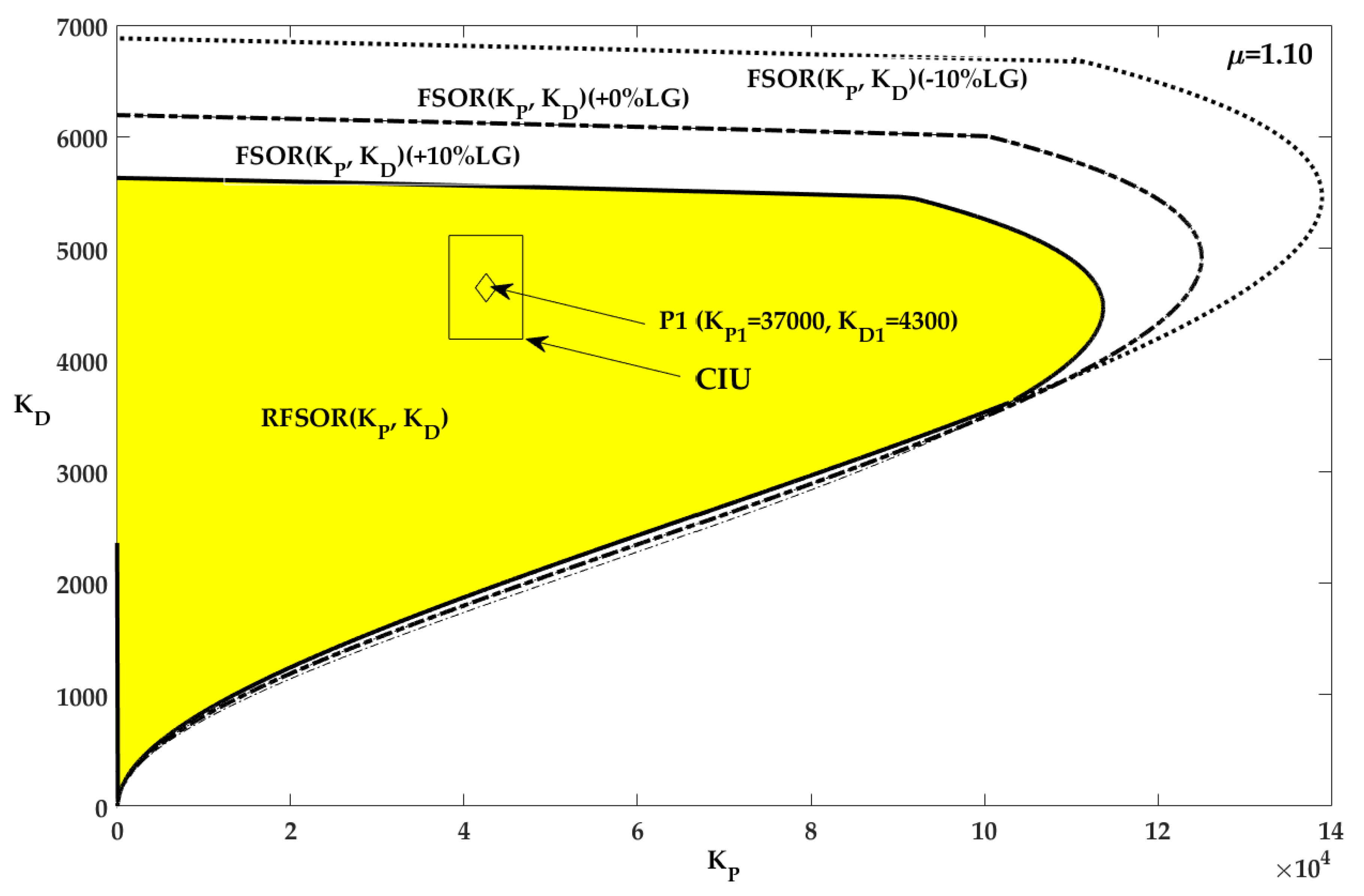
For robustness, variations in the control system are considered within a range of −/+10% for LG. These variations represent the unmodeled dynamics and parametric uncertainties of the electrical and mechanical terms of the SABSD system. Figure 13 shows the FSOR(K_P, K_D) region for −10%, +0%, and +10% LG variations. The intersection of these three regions defines the RFSOR(K_P, K_D) region. Within this region, the (K_P, K_D) controller sets ensure that the FOPD-controlled system meets the prespecified GM and PM specifications and maintains robustness in the presence of −10 to +10% LG variations.

To further compensate for the variations of the safety margins for the potential −10% to +10% controller implementation uncertainty (CIU), the RFOPD controller should be selected such that

$$\left(K_P, K_D\right)\subset \mathrm{RFSOR}(K_P, K_D),$$

(32)

and

$$(K_P\pm 10\%\ast K_P, K_D\pm 10\%\ast K_D)\subset \mathrm{RFSOR}(K_P, K_D).$$

(33)

For the IAE performance criteria, an optimal RFOPD controller, P1(K_P1 = 37,000, K_D1 = 4300), denoted as Case A, is selected from the RFSOR(K_P, K_D) of Figure 13. The rectangular region CIU, enclosing P1(K_P1 = 37,000, K_D1 = 4300), represents the potential −10% to +10% uncertainty in controller implementation.

For comparisons, in Case B, P2(K_P2 = 168.916, K_D2 = 176.686) is a traditional PD controller synthesized using the conventional root locus method [32]. This case represents the conventional controller frequently used in the position control of industrial SABSD systems. Case C denotes the original uncompensated system.

As for the implementation of this determined RFOPD controller, various approximation methods have been proposed in the literature. A detailed review of these methods is presented in [33]. This study uses the popular Oustaloup approach to approximate the determined RFOPD controller in both simulation and practical implementation studies. The lower and higher translation frequencies for approximation are ω_b = 0.001 rad/s and ω_h = 1000 rad/s; the approximation order is N = 5. The sampling time for the controller is set to 0.001 s.

4.2. Stability Analysis

To perform stability analysis, K_P, K_D, and μ = 1.10 of P1(K_P1 = 37000, K_D1 = 4300) are substituted into the open loop transfer function of Figure 11. The determined GM and PM for P1(K_P1 = 37,000, K_D1 = 4300) are 9.040 dB and 61.075 degrees, respectively. Thus, according to [24,25,26,27], the stability of the RFOPD-controlled SABSD system is guaranteed, and the pre-specified specifications are ensured. The computed GM and PM for Cases A, B, and C are all tabulated in

Table 2. Tuning parameters and performance comparison for Cases A, B, and C.

	Case A	Case B	Case C
Controller type	RFOPD controller	PD controller	Uncompensated system
Controller settings	P1(KP1 = 37,000, KD1 = 4300) μ = 1.10	P2(KP2 = 168.916, KD2 = 176.686)	None
Settling time (s)	0.105	5.013	25.061
Peak time (s)	0.051	3.755	18.781
IAE	0.031	8.632	6.153
ISE	0.021	3.677	4.505
IAEload	0.006	1.645	1.174
ISEload	0.001	1.451	3.029
GM (dB)	9.040	Inf	71.26
PM (Deg)	61.075	86.931	85.760

for comparison.

4.3. Simulation Studies

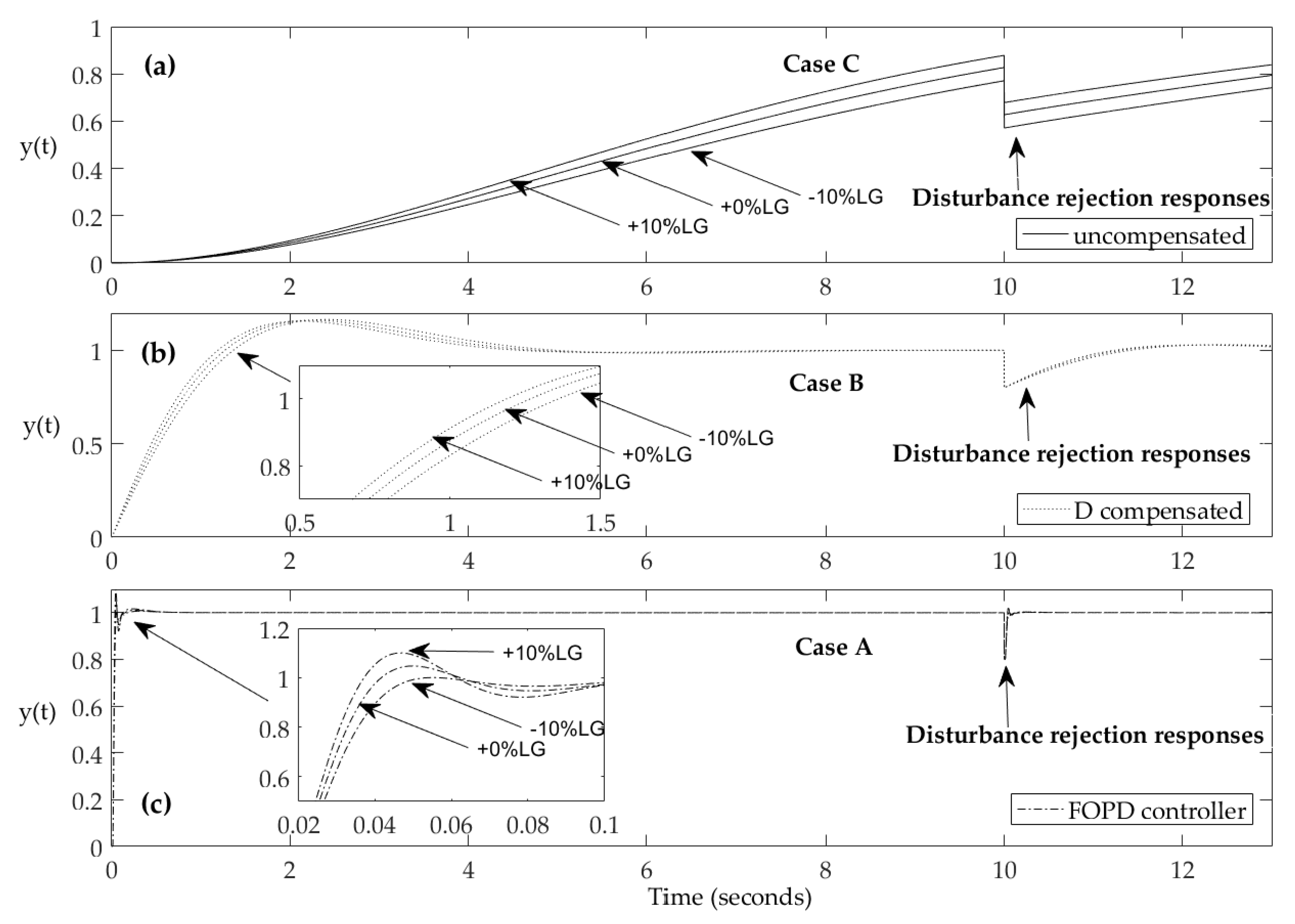
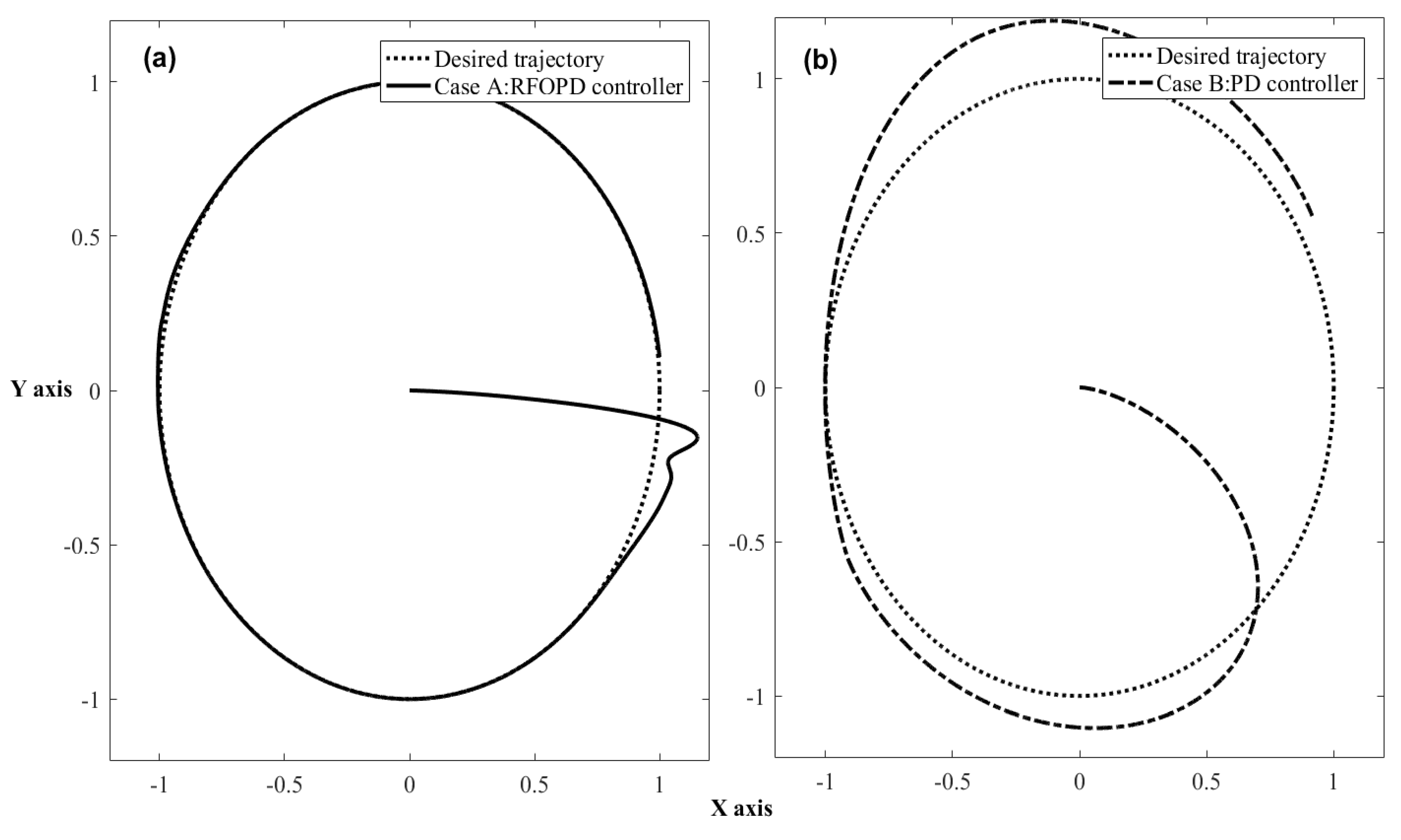
To evaluate the robustness of the three cases, we use Simulink to simulate the time responses. Figure 14 shows the unit step and disturbance responses for Cases A, B, and C subject to −10%, +0%, and +10% LG variations. Figure 15 shows the simulation studies for a round-type inspection for Cases A and B. Figure 14 and Figure 15 show that the proposed RFOPD controller gives satisfactory tracking and disturbance rejection responses in the presence of −/+10% LG variations. The time- and frequency-domain simulation results for these three cases are listed in Table 2.

As tabulated in Table 2, the proposed optimal RFOPD controller, P1(K_P1 = 37,000, K_D1 = 4300), not only satisfies the preassigned GM and PM constraints for robustness but also yields a faster tracking response, minimizing IAE, IAE_load, ISE, and ISE_load values. This demonstrates that the moving table and inspection pen of the SABSD system can be rapidly and accurately positioned. Additionally, the system exhibits robustness to loop gain variations, external disturbances, and uncertainties in controller implementation.

The SABSD systems for the X-stage and Y-stage have the same design but operate under different load conditions. As a result, both systems maintain robust stability and exhibit similar tracking and disturbance rejection responses.

5. Performance Evaluation

For performance evaluation, the determined RFOPD controller, P1(K_P1 = 37,000, K_D1 = 4300), is used for controlling the BSDXY stage of the ATPIS system shown in Figure 1. The robustness characteristics and contouring performances are experimentally examined in the presence of modeling uncertainties and disturbances. During inspections, the BSDXY stage is commanded to move the inspection pen along several pre-defined trajectories on the surface of the touch panels. These inspection trajectories include diagonal-line, rectangular-type, circular-type, convergent-type, round-type, and rhombus-type.

5.1. Robustness Verifications

All the values of the system parameters, listed in Table 1, are determined from the mechanical components’ experimental system or data sheets. As these parameters are used to formulate the mathematical model of the SABSD system, represented by Equation (17), there may be modeling uncertainties associated with these parameters due to variability in materials or experimental conditions.

To verify that the proposed RFOPD controller can overcome these modeling uncertainties and maintain robustness, it is applied to three BSDXY stages to perform rectangular-type inspections. Note that the X-stages, Y-stages, and their associated BLDC servo motors of these BSDXY stages are of the same model, but there may be parametric uncertainties present within them. The inspection results for these three stages are shown in

Table 3. Inspection results for the ATPIS system with three different BSDXY stages.

	BSDXY-A	BSDXY-B	BSDXY-C
Inspection type	rectangular-type	rectangular-type	rectangular-type
Inspection time (s)	2.390	2.406	2.390
Inspection trajectory

. It is evident that the ATPIS system demonstrates similar inspection trajectories with approximately the same inspection duration across the three BSDXY stages. This implies that the proposed RFOPD controller successfully overcomes the modeling uncertainties of the three employed BSDXY stages and retains robustness.

In another respect, in the standard mode, a digital PID controller, operating at a speed faster than the motion of the BSDXY stage and receiving the voltage signal from the transducer, is realized within the GUICS to maintain a constant interaction force between the IP and the touch panel during testing. However, the surface roughness of touch panels may result in varying degrees of friction forces between the IP and samples under examination, thereby influencing the positioning responses of the BSDXY stages. To observe the robustness of the RFOPD-controlled ATPIS system under disturbances caused by time-varying friction force conditions, three different IP–sample contact depths are investigated during diagonal-line inspections. Case depth_A denotes the aforementioned standard mode. In Case depth_B and Case depth_C, the inspection pen is moved closer to the touch panel than the standard mode by 50 μm and 100 μm, respectively. Note the minimum resolution for the inspection pen in the Z-axis, mounted on the Z-stage with a five-phase stepping motor, is 2 μm.

Table 4. Inspection results for the ATPIS system with three different IP–sample contact depths.

	Case depth_A	Case depth_B	Case depth_C
Inspection type	diagonal-line	diagonal-line	diagonal-line
IP–sample contact depth	standard mode	50 μm	100 μm
Inspection time (s)	0.756	0.750	0.759
Inspection trajectory

presents the inspection results for three cases with different contact depths. The trajectories and durations for the specified diagonal-line inspection are approximately the same. These observations imply that the disturbance induced by friction forces does not significantly impact the tracking responses of the inspection pen. Therefore, the ATPIS system with the proposed RFOPD controller maintains robustness in the presence of frictional forces and produces rapid and satisfactory inspection results.

5.2. Performance Comparisons

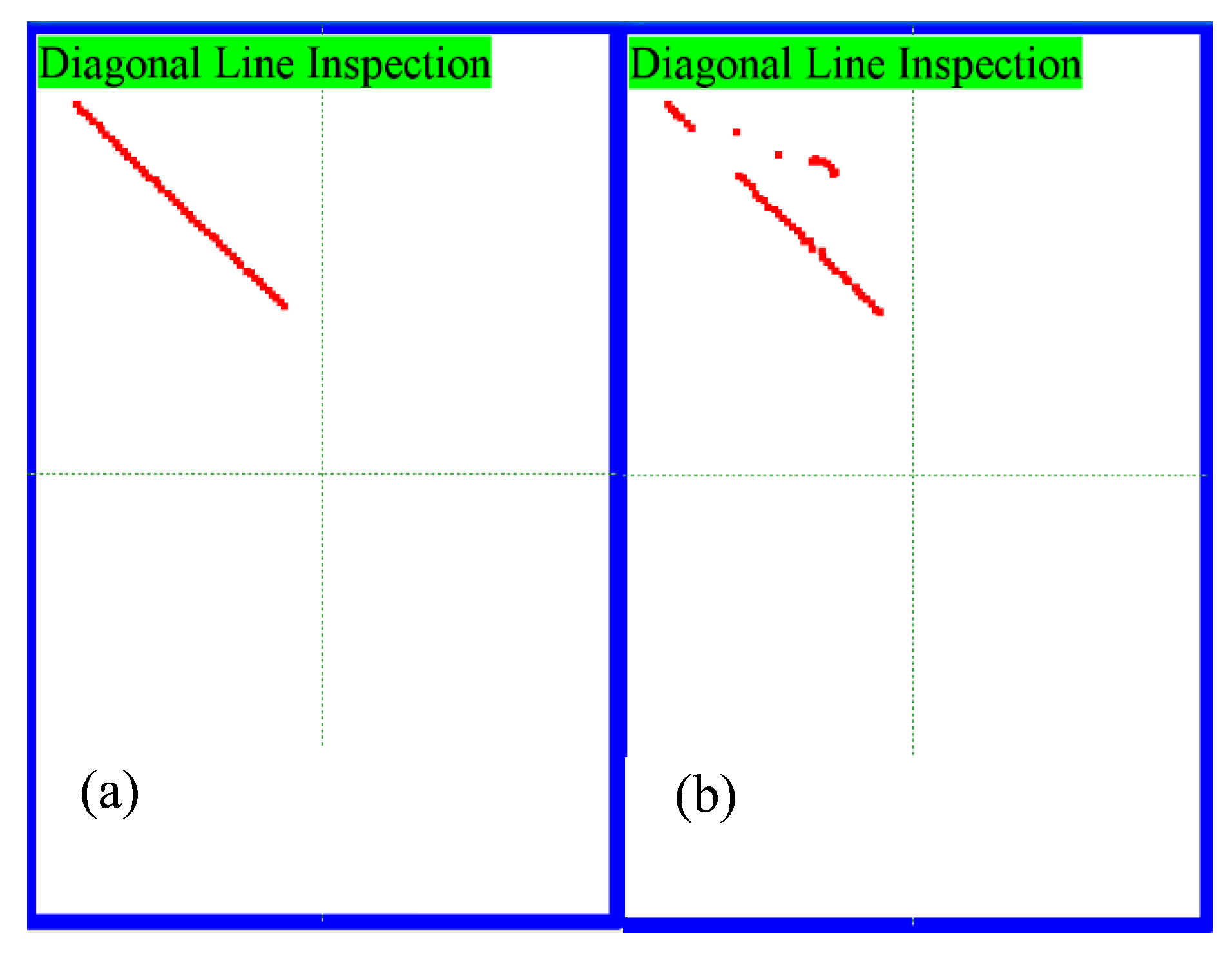
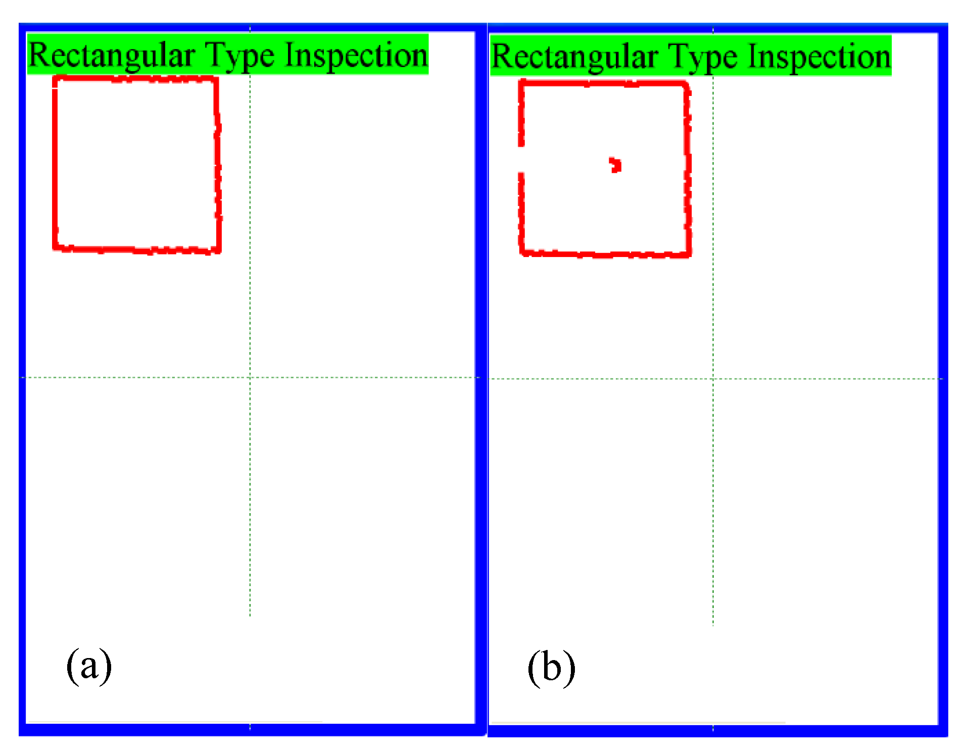
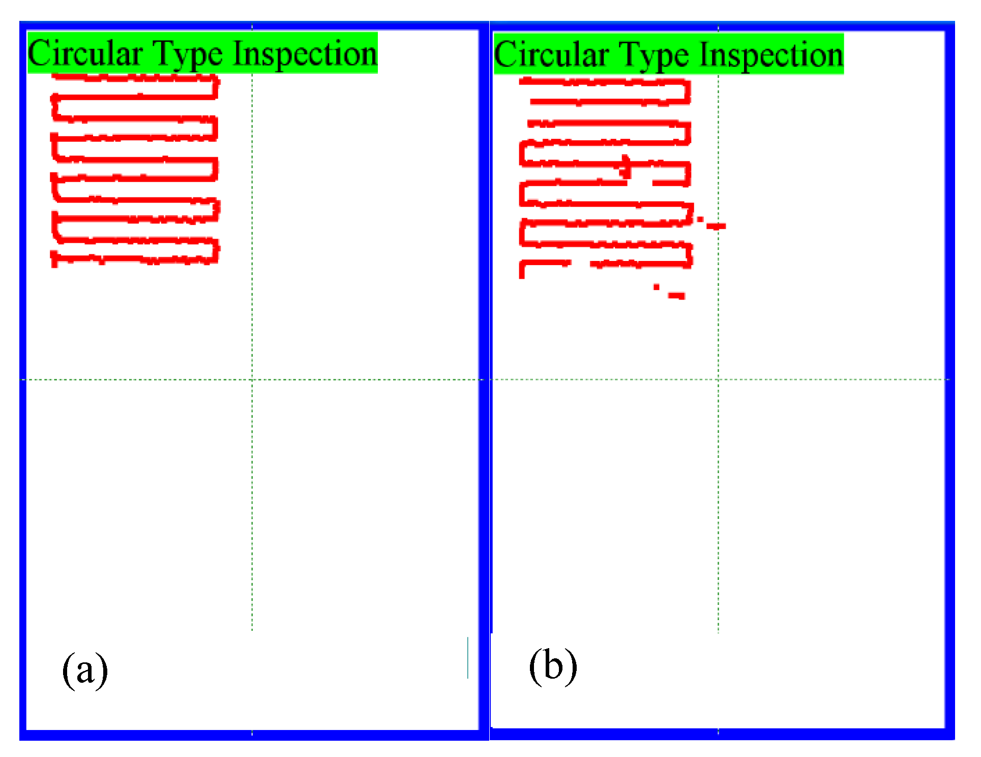
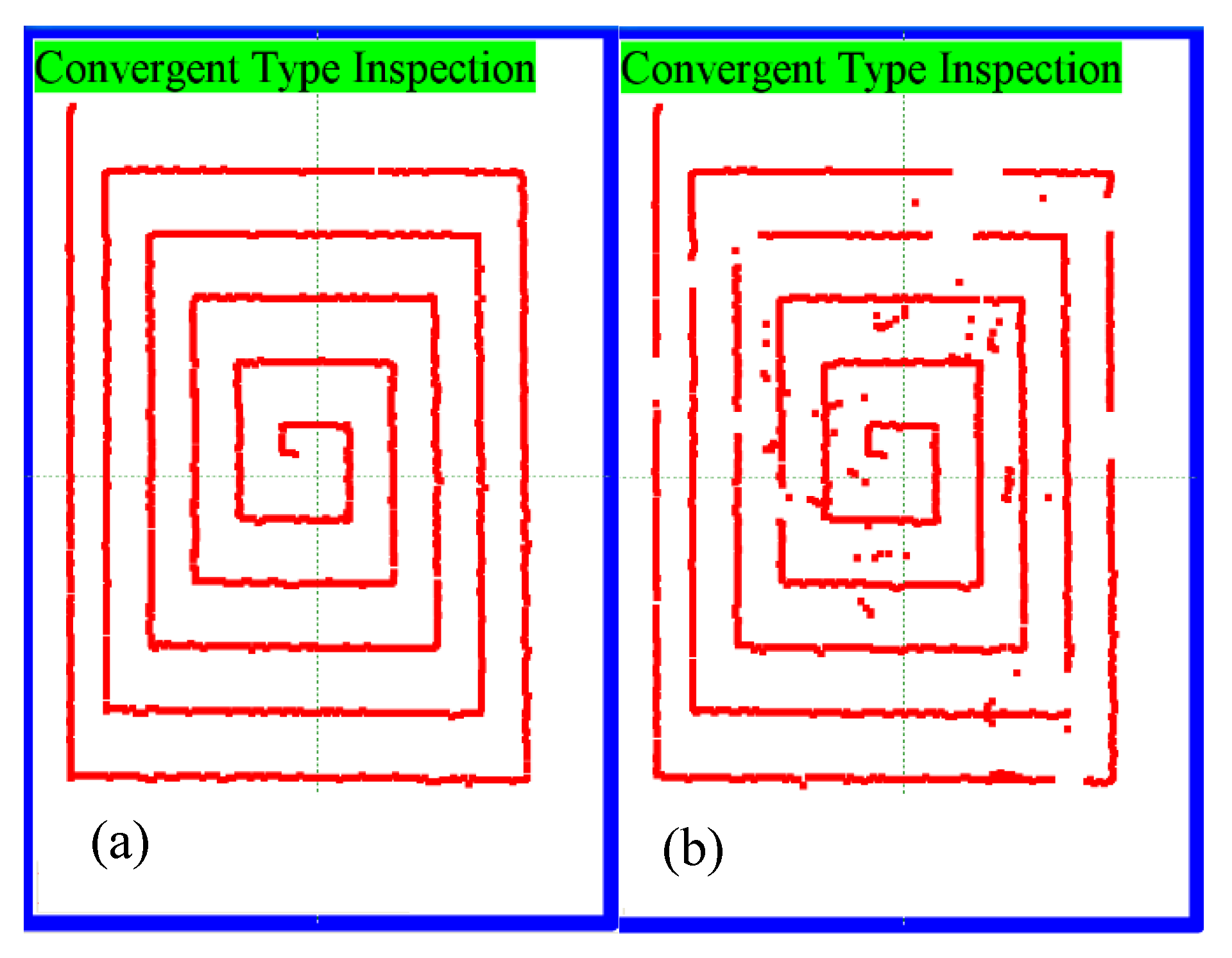
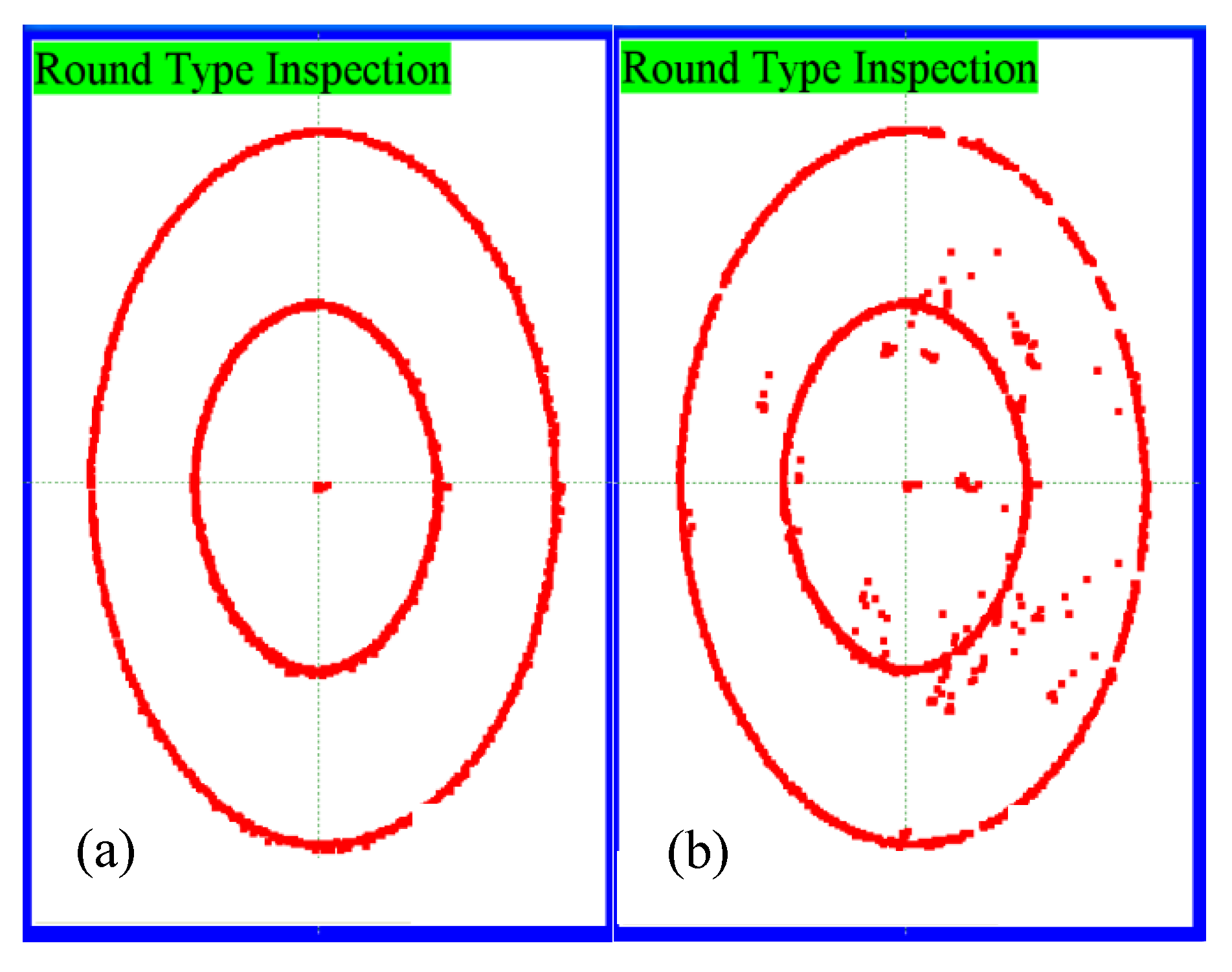
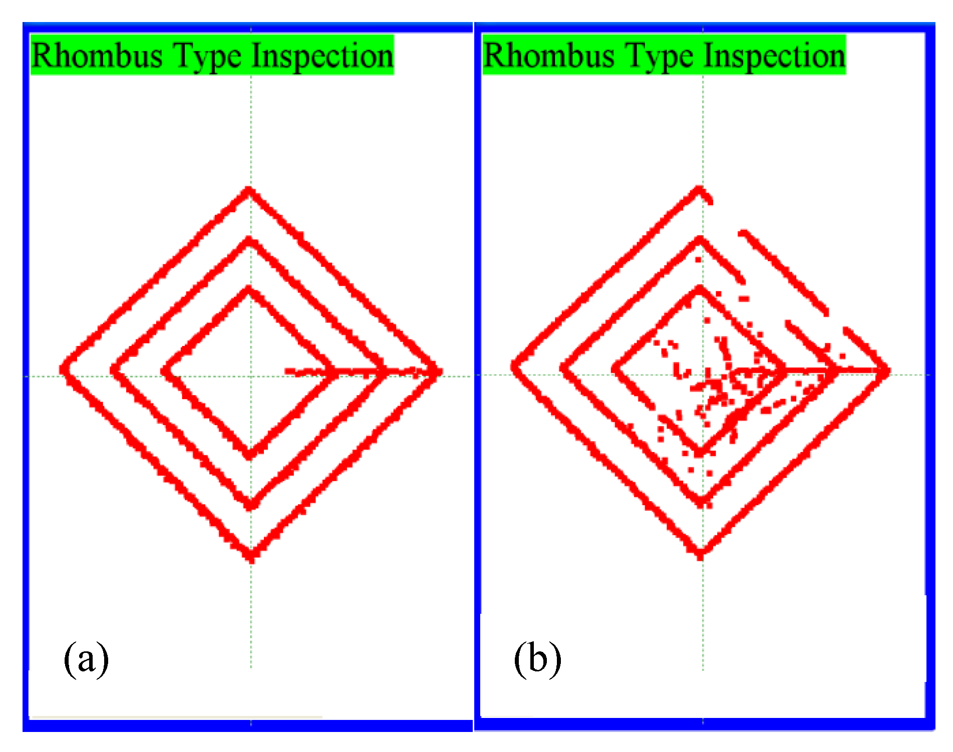
The results for various types of inspections are illustrated in Figure 16, Figure 17, Figure 18, Figure 19, Figure 20 and Figure 21. Figure 16a, Figure 17a, Figure 18a, Figure 19a, Figure 20a and Figure 21a indicate a pass for the inspection, as the red detected inspection trajectories are continuous and coincide with the pre-specified trajectories. These figures also confirm that the mechanical couplings between the two axes of the BSDXY stage are minimal and can be disregarded. In addition, Figure 16b, Figure 17b, Figure 18b, Figure 19b, Figure 20b and Figure 21b show discontinuous trajectories, so these inspections fail. These discontinuous points show the existence of possible defects at these points.

Table 5. The time required to achieve a pass inspection for Cases A and B.

	Case A	Case B
Diagonal-line	0.750 s	2.735 s
Rectangular-type	2.407 s	8.665 s
Circular-type	6.672 s	20.684 s
Convergent-type	18.125 s	59.812 s
Round-type	25.797 s	85.130 s
Rhombus-type	29.688 s	103.908 s

shows the time needed for a pass inspection for Cases A and B. Case B gives slower responses, so a longer time is required to achieve an acceptable inspection. It is evident that the inspection time for proposed Case A is significantly shorter for all six inspection trajectories. Due to paper length limitations, the inspection trajectories for Case B are excluded.

These inspection results demonstrate that when the ATPIS system with the BSDXY stage is controlled using the proposed RFOPD controller, it successfully performs inspections for diagonal-line, rectangular-type, circular-type, convergent-type, round-type, and rhombus-type. The proposed RFOPD controller accurately and rapidly utilizes the BSDXY stage to move the inspection pen to any specified point on the surface of touch panels, significantly reducing the inspection time. In addition, the RFOPD-controlled ATPIS system maintains robustness in the presence of modeling uncertainties and disturbances induced by time-varying friction forces.

6. Conclusions

This study designs and implements an optimal RFOPD controller to improve the tracking and disturbance rejection responses of ATPISs and significantly reduce the inspection time for TPs. The TDOS, consisting of a BSDXY stage driven by two BLDC servo motors and one compact linear actuator powered by a five-phase stepping motor, is designed and implemented to move the IP vertically or horizontally. A TPI system immediately determines the touch point and converts the coordinates into voltage signals.

By employing the mechanical and dynamical parameters of the TDOS, the transfer function that relates the voltage inputs of the BLDC servo motors to the position of the BSDXY stage is determined. The GPMT tester and stability equation methods graphically characterize the FSOR(K_P, K_D) region for −10%, +0%, and +10% LG variations. An RFSOR(K_P, K_D) region is determined, enclosing all the admissible RFOPD controller sets. These controller sets ensure that the FOPD-controlled system meets the prespecified GM and PM specifications and maintains robustness subject to −10 to +10% LG variations.

The RFOPD controller, P1(K_P1 = 37,000, K_D1 = 4300), is chosen from the RFSOR(K_P, K_D) based on the minimum IAE value. This selection considers potential uncertainties in controller implementation ranging from −10% to +10%. The computed GM and PM for P1(K_P1 = 37,000, K_D1 = 4300) are 9.040 dB and 61.075 degrees, respectively, guaranteeing the stability of the RFOPD-controlled SABSD system. Matlab-based computer simulations confirm the effectiveness of the RFOPD controller, featuring more rapid tracking and disturbance rejection responses than the traditional PID controller designed using the root locus method.

For practical verification, a GUICS is developed in Borland C++ Builder 10.0 on Windows 10 to perform diagonal-line, rectangular-type, circular-type, convergent-type, round-type, and rhombus-type inspections. The homemade GUICS also automatically executes and validates reliability and touch pressure tests.

The inspection results show that the ATPIS with the proposed RFOPD controller causes the IP to track an operator-defined inspection trajectory accurately and rapidly. As a result, the inspection time is reduced to about one-third compared to the ATPIS using a traditional PID controller. The robustness of the RFOPD-controlled ATPIS subject to unmodeled uncertainties and friction-induced disturbance is verified in simulation and experimental studies. The proposed ATPIS conducts fast and reliable in-line inspection of small- or middle-scale TPs. The system accommodates objective measurements, enabling a shorter production cycle and improved production quality through the capability for multiple rapid inspections.

References

- Chen, Y.C.; Yu, J.H.; Shiou, F. Automated optical inspection system for analogical resistance type touch panel. Int. J. Phys. Sci. 2011, 6, 5141–5152. [Google Scholar]
- Lin, H.D.; Tsai, H.H. Automated quality inspection of surface defects on touch panels. J. Chin. Inst. Ind. Eng. 2012, 29, 291–302. [Google Scholar] [CrossRef]
- Chiang, Y.M.; Lin, Y.L.; Chien, W.H. Automated surface defect inspection system for capacitive touch sensor. In Proceedings of the 2015 7th International Conference of Soft Computing and Pattern Recognition, Fukuoka, Japan, 13–15 November 2015; pp. 274–277. [Google Scholar] [CrossRef]
- Ye, R.; Chang, M.; Pan, C.S.; Chiang, C.A.; Gabayno, J.L. High-resolution optical inspection system for fast detection and classification of surface defects. Int. J. Optomechatron. 2018, 12, 1–10. [Google Scholar] [CrossRef]
- Li, C.; Pan, H.; Cai, J.; Chen, X. Defects detection of mobile phone touch screen circuit based on machine vision. In Proceedings of the 2020 Chinese Automation Congress (CAC), Shanghai, China, 6–8 November 2020; pp. 1–5. [Google Scholar] [CrossRef]
- Jenkinson, R. Touch Screen Testing Platform Having Components for Providing Conductivity to a Tip. U.S. Patent No. 9,652,077B2, 16 May 2017. [Google Scholar]
- Verma, P.; Chauhan, D.S.; Ramaswamy, R.; Likith Kumar, C. Multi-touch testing robot. Int. J. Control Theory Appl. 2017, 10, 219–223. [Google Scholar]
- Wilson, A.; Aronin, P.; Akhil, A. Robot Arm for Testing of Touchscreen Applications. Patent No. WO2017051263, 2017. World Intellectual Property Organization. Available online: https://patentscope.wipo.int/search/en/detail.jsf?docId=WO2017051263 (accessed on 4 February 2024).
- Lu, C.C.; Juang, J.G. Robotic-based touch panel test system using pattern recognition methods. Appl. Sci. 2020, 10, 8339. [Google Scholar] [CrossRef]
- Frister, D.; Goranov, A.; Oberweis, A. Automated testing of mobile applications using a robotic arm. In Proceedings of the 2020 International Conference on Computational Science and Computational Intelligence, Las Vegas, NV, USA, 16–18 December 2020; pp. 1729–1735. [Google Scholar] [CrossRef]
- IAI America, Inc. (n.d.). Automating Touch Panel Inspection Process. Available online: https://www.intelligentactuator.com/automating-touch-panel-inspection-process/ (accessed on 13 August 2023).
- Wang, Y.J. Design and implementation of a rapid automated defects inspection system for resistive touch panels with a PID-like fuzzy controller. In Proceedings of the 2015 34th Chinese Control Conference, Hangzhou, China, 28–30 July 2015; pp. 8685–8691. [Google Scholar] [CrossRef]
- Bechlioulis, C.P.; Rovithakis, G.A. Robust adaptive control of feedback linearizable MIMO nonlinear systems with prescribed performance. IEEE Trans. Autom. Control 2008, 53, 2090–2099. [Google Scholar] [CrossRef]
- Zhang, J.X.; Yang, G.H. Fuzzy Adaptive output feedback control of uncertain nonlinear systems with prescribed performance. IEEE Trans. Cybern. 2018, 48, 1342–1354. [Google Scholar] [CrossRef]
- Zhang, J.X.; Wang, Q.G.; Ding, W. Global output-feedback prescribed performance control of nonlinear systems with unknown virtual control coefficients. IEEE Trans. Autom. Control 2022, 67, 6904–6911. [Google Scholar] [CrossRef]
- Podlubny, I. Fractional-order systems and PIλDμ controllers. IEEE Trans. Autom. Control 1999, 44, 208–214. [Google Scholar] [CrossRef]
- Ruszewski, A. Stability regions of closed loop system with time delay inertial plant of fractional order and fractional order PI controller. Bull. Pol. Acad. Sci. Tech. Sci. 2008, 56, 329–332. [Google Scholar]
- Hamamci, S.E.; Koksal, M. Calculation of all stabilizing fractional-order PD controllers for integrating time delay systems. Comput. Math. Appl. 2010, 59, 1621–1629. [Google Scholar] [CrossRef]
- Wang, Y.-J.; Huang, S.-T.; You, K.-H. Calculation of robust and optimal fractional PID controllers for time delay systems with gain margin and phase margin specifications. In Proceedings of the 2017 36th Chinese Control Conference, Dalian, China, 26–28 July 2017; pp. 3077–3082. [Google Scholar] [CrossRef]
- Keyser, R.D.; Muresan, C.; Ionescu, C. A novel auto-tuning method for fractional order PI/PD controllers. ISA Trans. 2016, 6, 268–275. [Google Scholar] [CrossRef] [PubMed]
- Li, C.; Zhang, N.; Lai, X.; Zhou, J.; Xu, Y. Design of a fractional-order PID controller for a pumped storage unit using a gravitational search algorithm based on the Cauchy and Gaussian mutation. Inform. Sci. 2017, 396, 162–181. [Google Scholar] [CrossRef]
- Zhao, C.N.; Xue, D.Y.; Chen, Y.Q. A fractional order PID tuning algorithm for a class of fractional order plants. IEEE Int. Conf. Mechatron. Autom. 2005, 1, 216–221. [Google Scholar] [CrossRef]
- Valerio, D.; Sa da Costa, J. Tuning of fractional PID controllers with Ziegler–Nichols-type rules. Signal Process. 2006, 86, 2771–2784. [Google Scholar] [CrossRef]
- Chang, C.H.; Han, K.W. Gain margins and phase margins for control systems with adjustable parameters. J. Guid. Control Dyn. 1990, 13, 404–408. [Google Scholar] [CrossRef]
- Huang, Y.J.; Wang, Y.J. Robust PID tuning strategy for uncertain plants based on the Kharitonov theorem. ISA Trans. 2000, 39, 419–431. [Google Scholar] [CrossRef] [PubMed]
- Wang, Y.J. Graphical computation of gain and phase margin specifications-oriented robust PID controllers for uncertain systems with time-varying delay. J. Process Control 2010, 21, 475–488. [Google Scholar] [CrossRef]
- Han, K.W. Analysis of robust control systems using stability equations. J. Control Syst. Technol. 1993, 1, 83–89. [Google Scholar]
- Huang, S.J.; Wang, S.S. Mechatronics and control of a long-range nanometer positioning servomechanism. Mechatronics 2019, 19, 14–28. [Google Scholar] [CrossRef]
- Zhou, C.G.; Feng, H.T.; Chen, Z.T.; Ou, Y. Correlation between preload and no-lad drag torque of ball screws. Int. J. Mach. Tools Manuf. 2016, 102, 35–40. [Google Scholar] [CrossRef]
- Fukada, S.; Fang, B.; Shigeno, A. Experimental analysis and simulation of nonlinear microscopic behavior of ball screw mechanism for ultra-precision positioning. Precis. Eng. 2011, 35, 650–668. [Google Scholar] [CrossRef]
- Yan, Y.; Yang, J.; Sun, Z.; Zhang, C.; Li, S.; Yu, H. Robust speed regulation for PMSM servo system with multiple sources of disturbances via an augmented disturbance observer. IEEE/ASME Trans. Mechatron. 2018, 23, 769–780. [Google Scholar] [CrossRef]
- Nise, N.S. Control Systems Engineering, 7th ed.; John Wiley & Sons: San Francisco, CA, USA, 2015. [Google Scholar]
- Vinagre, B.M.; Podlubny, I.; Hernandez, A.; Feliu, V. Some approximations of fractional order operators used in control theory and applications. Fract. Calc. Appl. Anal. 2000, 3, 231–248. [Google Scholar]
Figure 1.
A photo of the homemade ATPIS.
Figure 2.
The general structure of 5-wire resistive TPs.
Figure 3.
The internal structure of general surface capacitive TPs.
Figure 4.
The internal structure of general projected capacitive TPs.