Abstract
The widespread availability of tools to collect and share spatial data enables us to produce a large amount of geographic information on a daily basis. This enormous production of spatial data requires scalable data management systems. Geospatial architectures have changed from clusters to cloud architectures and more parallel and distributed processing platforms to be able to tackle these challenges. Peer-to-peer (P2P) systems as a backbone of distributed systems have been established in several application areas such as web3, blockchains, and crypto-currencies. Unlike centralized systems, data storage in P2P networks is distributed across network nodes, providing scalability and no single point of failure. However, managing and processing queries on these networks has always been challenging. In this work, we propose a spatio-temporal indexing data structure, DSTree. DSTree does not require additional Distributed Hash Trees (DHTs) to perform multi-dimensional range queries. Inserting a piece of new geographic information updates only a portion of the tree structure and does not impact the entire graph of the data. For example, for time-series data, such as storing sensor data, the DSTree performs around 40% faster in spatio-temporal queries for small and medium datasets. Despite the advantages of our proposed framework, challenges such as 20% slower insertion speed or semantic query capabilities remain. We conclude that more significant research effort from GIScience and related fields in developing decentralized applications is needed. The need for the standardization of different geographic information when sharing data on the IPFS network is one of the requirements.
1. Introduction
With the advancement of Internet-based services and sensors, such as the widespread adoption of GPS (Global Positioning System)-based sensors, location-based services, improvements in computational data processing, and satellite imagery, a large amount of novel spatial information is produced daily [1]. The widespread availability of tools to collect and share spatial data enables individuals and small communities to produce their own digital spatial content (e.g., Open Street Maps contributions have tripled between 2012 and 2017 [2]). This enormous production of spatial data requires scalable data management systems [3]. The data infrastructure technology supporting spatial data management and processing has changed from standalone relational database systems to spatial data warehouses that support a variety of data formats and analytical workloads [4] and from centralized infrastructures to decentralized and peer-to-peer (P2P) systems. In addition to the new system architectures, new data structures have been proposed such as, e.g., HDF [5], Data-Cubes [6], Geoparquet [7], and spatial data management and analytic frameworks (e.g., Apache iceberg [8], Digital Earth [9]) have emerged to manage and perform analysis on large-scale, high temporal and spatial resolutions.
Geospatial architectures are another area of technological change developed to handle spatial data management challenges. They have changed from clusters to cloud architectures and more parallel and distributed processing platforms (e.g., Spark [10], Hadoop [11]). In the realm of network and application architecture, P2P systems have been established in several application areas. In the past decade, P2P systems have been used widely in web3 [12], blockchains [13], and crypto-currencies [14]. The combination of P2P file-sharing systems with blockchains provides scalability, security, immutability, and append-only attributes for sharing information amongst nodes on a network [15]. These attributes make P2P networks suitable for content distribution and service discovery applications [16,17,18,19]. However, the main limitation of existing systems is they can only locate data on the network based on a key value using DHT [20]. While DHTs have been used as a main building block for P2P applications, they are seriously deficient in one regard; they only directly support exact match queries and do not allow users to query data by range requests [21,22,23,24]. The multi-dimensionality of spatio-temporal data is one of the big challenges in retrieving and querying these data in P2P networks. When querying spatio-temporal data, the ability to perform range queries is required, and it is not currently supported. The rapid increase in spatio-temporal data collection needs a new auxiliary indexing structure. These indexing structures are responsible for tracking the behavior of moving objects through space [25,26]. These indexing methods allow P2P architectures to find and retrieve contents based on the user’s filters and address more complex data sharing needs, facilitating data management, query processing, and delivering data to the end-user.
While much work has been carried out towards expediting search in file-sharing P2P systems, issues concerning spatial indexing in P2P systems are significantly more complicated due to cases such as overlaps between spatial objects, avoidance of data scattering, and the complexity of spatial queries [27]. One-dimensional data mainly have been queried using DHTs in P2P networks [28,29,30]. DHTs are not yet designed for complex spatial queries (e.g., range query, k-nearest neighbor query), and only support the location of data items based on a key value (i.e., equality lookups) [20,31]. For multi-dimensional data, there have been multiple approaches; the first approach includes partitioning data into one-dimensional indexes using space-filling curves or kd-tree-based methods and indexing them using DHT methods (e.g., [32,33,34]). These methods usually work best with static data, and dynamic content relocation (locality) is dependent on the accuracy of the space-filling curves [34].
Another approach to apply range queries to the P2P networks is to use multiple DHTs in the network (e.g., [35,36,37]). This method needs a higher level of network and node structure manipulation and is not commonly used in large-scale projects due to interoperability limitations of this approach [38]. A third approach is to construct traditional indexes that have been used in centralized environments and distribute these indexes on the P2P network (e.g., [20,21,39,40]). This approach is implemented by constructing a tree and splitting it into parts and maintaining parts of semi-independent trees at each peer. Prefix Hash Tree (PHT) [21] and, similarly, P-Tree [20] use the same approach by storing a fraction of the overall tree on each peer. In PHT, each node of the tree is labeled with a prefix which is defined recursively. Given a node with the label l, its left and right children are labeled as and , respectively. This pattern constructs a tree structure and enables range queries on a dataset [21].
In this work, we propose a spatio-temporal indexing data structure that works in the data layer and uses a distributed InterPlanetary File System (IPFS) network. Our method is closer to the approach of Ranabhadran et al. [21] and does not require additional DHTs to perform multi-dimensional range queries. The rest of this paper is divided into two main sections. First, we introduce the Distributed Spatio-Temporal Tree (DSTree) as a data structure to perform range spatio-temporal queries on a dataset and we check its features and performance by comparing it to other existing trees. Second, we will look at the integration of DSTree with distributed networks and propose a system architecture to perform queries on the IPFS using DSTree. The originality of this work includes the ability of the spatio-temporal queries on the data shared on IPFS system. This sort of query allows sharing and querying spatio-temporal data on P2P systems without the need for any third-party central entities.
2. Spatio-Temporal Data Indexing Methods
P2P multidimensional query processing refers to the execution of advanced query operators over multidimensional data stored in a distributed system [41]. The retrieved data from a query should be exact and complete. Exactness means the query result should not be approximate. The retrieved data should exactly belong to the query results set. This means that if we run a query on the same dataset on a centralized system, the results should be exactly the same as when we run a query on the distributed system. A basic element of geospatial technology can be defined as three main components including location in space and time, and attribute of that location in space-time [42]. In this work, our focus is to address a methodology to allow users to retrieve a geographic object based on space or time queries from a P2P network.
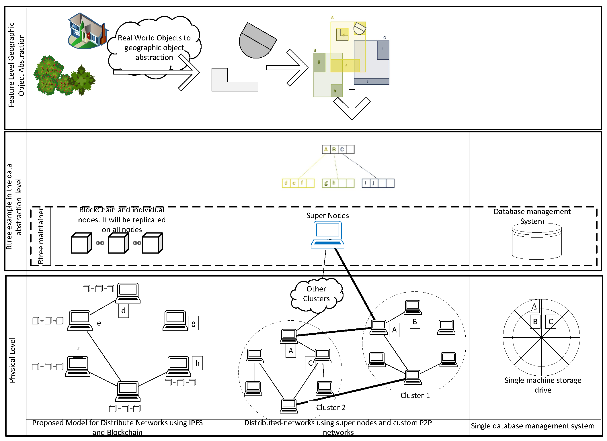
The spatio-temporal indexing methods in central systems are mainly performed at an abstract level (Figure 1). They are used to improve query performance on the datasets. These indexes usually work as a separate layer on top of the data layer itself. Queries are usually performed against the indexes and then the actual reference to the geographic features are then retrieved from the index. In contrast, our method stores data on the nodes on the network using spatial indexing methods in both abstract and physical storage layers. For example, the purpose of indexing can also be to distribute data that are closer in space, on the nodes that are closer in the network [20] (Figure 1, middle). Through the last couple of decades, many spatio-temporal access methods have been developed. There have been several approaches for spatio-temporal indexing so far [25,26,43,44,45,46,47,48]. Handling temporal data in GIS ranges from time-stamping GIS layers [49], to more object-oriented approaches such as time-stamping events and processes [44,50]. Another category of spatio-temporal models is trajectory-based access models which track the changes in the geographic object typologies over time [47]. In central systems, indexing models such as Oct-tree [51] are sometimes used to process spatio-temporal queries [47,52,53]. In using Oct-trees for indexing spatial data, each geographic object is considered as a cuboid. The spatial dimension of the data is considered as two dimensions of each cuboid. The third dimension of a cuboid is considered a time interval. There have been some newer approaches to the query process of spatio-temporal data using blockchains. For example, ref. [54] used a block-DAG-based index traversal algorithm to handle spatio-temporal queries on a block-DAG. However, the main issue with the blockchain-based spatial–temporal indexes is the limited data storage capability on the blockchains [55].
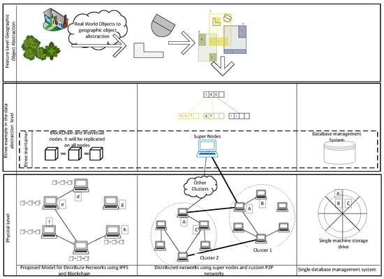
Figure 1.
Abstraction levels of geographic information. Spatial indexes cluster units of Geographic Information (GI) at the abstract level and it is used at the storage level in the different architectures. The Spatial Index maintenance is handled by RDBMS [56] (Left) or super nodes (Middle) in some studies [20], or using proposed blockchain-based method (Right). In the proposed model, each node maintains a spatial index and the latest version of the index is always published on the blockchain. Each node only stores and serves features that they need using IPFS. Rows show different abstraction levels of geographic information from real-world phenomena to machine language.
A decentralized spatial indexing technique must be scalable enough to be able to handle hundreds of thousands of peers and also dynamic enough to deal with peers joining/leaving the system anytime. Another feature of such structures is their ability to preserve the locality and directionality of multidimensional information. Locality implies that multidimensional information is stored in neighboring nodes, while directionality implies that the index structure preserves orientation. The notions of locality and directionality are very important. If an index structure preserves these properties, then searching in the index corresponds to searching in the multidimensional space, which can highly improve query evaluation cost [27]. R-tree-based indexes can efficiently answer various types of multidimensional queries, especially range queries [57]. In addition, a spatio-temporal indexing method is required to support two types of topological relations. The first set of topological relations includes temporal typologies which are based on Allen’s temporal algebra covered in [58,59]. These relations include seven typologies that are briefly explained in Table 1. A time interval for Geographic Information (GI) can be defined as the duration in which a GI feature exists with a fixed state. This interval can be as small as a few milliseconds that it takes to collect a GI feature or can be a considerably longer time period, such as geological land classifications or land cover. Defining time intervals and how a GI can be attached to a newer time interval depends on the context of the study. The second type of topological relations which needs to be addressed by a spatio-temporal indexing model is spatial topology.

Table 1.
Temporal algebra introduced by [58]. X (line border) is time interval of the first GI and Y (dashed border) is the time interval of the second GI.
Each indexing method is optimized for specific types of queries. Our proposed method is more suitable for the storage, query processing, and retrieval of log-based data. These data are produced over the time that different events happen. An example of such data is data that are being collected from a sensor over time or a VGI tool to share images from different locations by users or even open data which are being shared by different government departments, such as crime data that are being shared by the police. Each of these datasets can have different access levels, and geoprivacy levels are being collected over time.
DSTree is a two-level tree structure. The approach of DSTree is close to the work carried out by [60,61,62]. They constructed a multilevel tree structure to improve the query process of trajectory data. In the method developed by [60], they formed a global space-time subdivision scheme. Sun et al. combined two trees, an R*-Tree and a kd-Tree, to improve the query process on the centralized machines [61]. Tao [62] also used a series of temporal quad-Trees to handle interval queries in centralized systems. In a DSTree, an Interval-Tree [63,64] is used as the top part of the tree, and a quad-Tree [65] is used at the bottom part of the tree.
3. Dstree: A Spatio-Temporal Index
A unit of GI in our model is defined as a spatio-temporal object which can be represented in the form of
where is the identification of the object. GI is geographic location, including longitude and latitude along x and y dimensions. is Minimum Boundary Rectangle (MBR), which is constructed based on its location. is the temporal interval the is valid during. Each also has a set of attributes, p, associated with it.
The interval tree is responsible for temporal queries and the quad-Tree is responsible for performing the spatial part of the queries. We define a time interval as a pair of real numbers where . can be represented as . Different variants of the interval trees are capable of supporting open and half-open intervals. Interval trees are optimized for querying of intervals which overlap with a given interval, but can also be used for point queries. Having the ability to query overlapping intervals allows us to query based on the temporal topology in Table 1. During each time interval, we assume that the GI state does not change.
3.1. Dstree Index
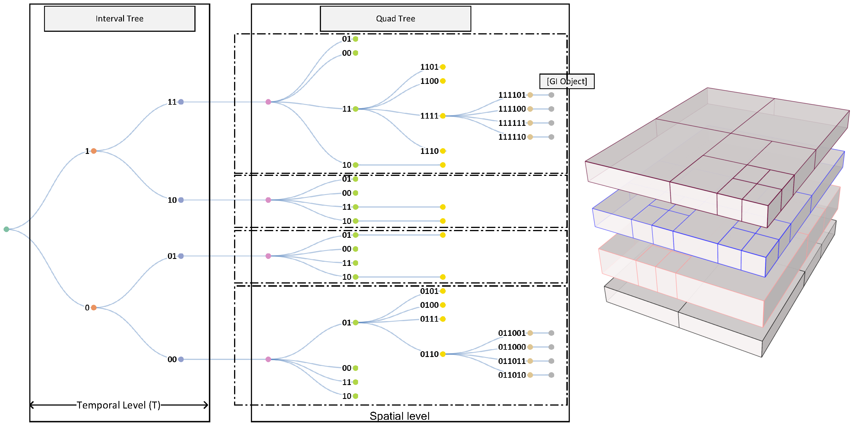
When constructing a DSTree, it is possible to partition data into spatio-temporal chunks and assign a unique ID to each portion of the data. The proposed DSTree indexes are composed of two parts, as shown in Figure 2. The first component (A) is called the interval tree index, and the second component (B) is called the quad index. The interval tree is a binary tree so each node can have only two children. By assigning 1 to the right child and 0 to the left child, a series of IDs will be constructed. The length of digits in the interval tree portion of the index equals the temporal level (T). The second section of the DSTree index is a quad index. Each node in a Quad-tree consists of four children. Each child can be assigned an index from 00, 01, 10, and 11 and it can construct the quad index. Figure 3 shows the DSTree index corresponding to quad-tree indexes.
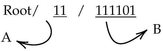
Figure 2.
An example of DSTree Index. Each index is constructed of two sub-parts. Part A is the interval tree index. Its length is equal to the temporal level (T). Part B is the quad-tree index.
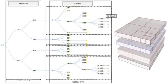
Figure 3.
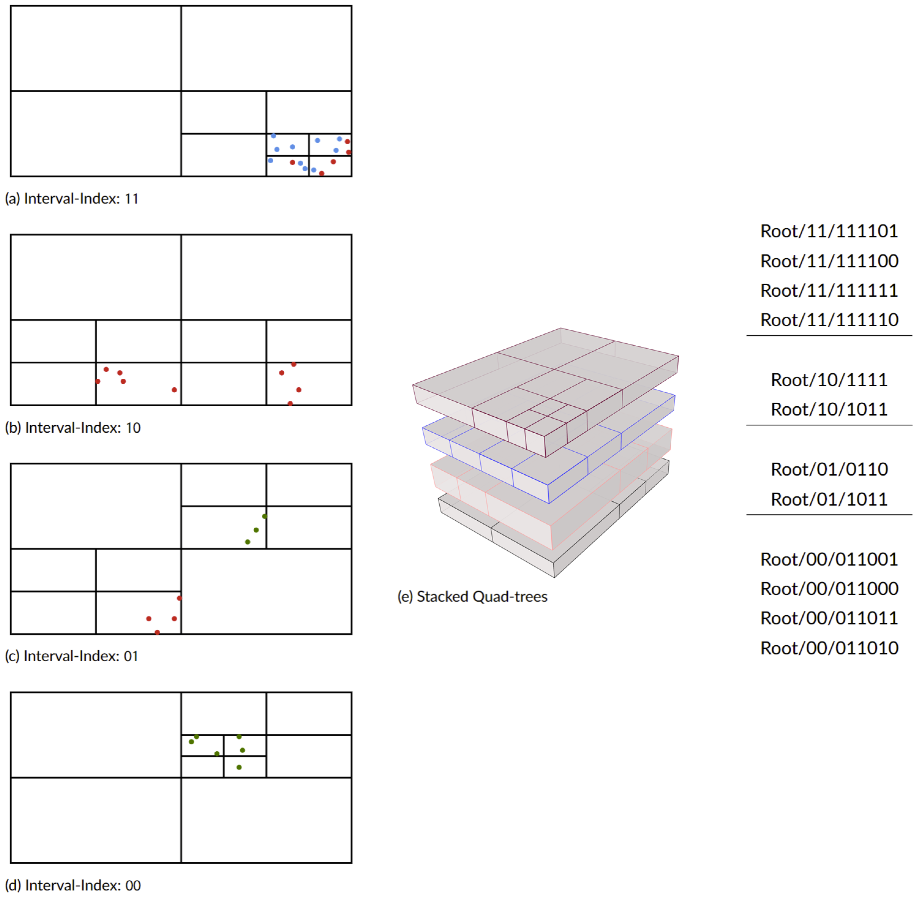
An example of DSTree constructed from a set of sample points. Each DSTree has a temporal (interval tree) component and a spatial (quad-tree) component. The final graph will be a stack of quad-trees on top of each other. Spatial level is the number of levels in the quad-tree.
The top part of the DSTree is a regular interval tree. However, the depth of this tree is controlled by a parameter called temporal level (T). T is responsible for balancing between the top-level tree and the bottom-level tree. Once the top interval tree is constructed, the GI in the leaves (each leaf includes n GI) is used to construct a quad-tree. As a result, we will have one quad-tree at each leaf of the interval tree at the level of T. Regular quad-trees always have an extent equal to the minimum boundary box of the GI inserted into the tree. However, in a DSTree, all of the quad-trees should have the same extent, e.g., equal to in geographic coordinates. Having the same spatial extent, the bottom part of DSTree allows us to query data across all of the interval tree leaves. Figure 3 shows an example of a constructed DSTree. Figure 4 shows the points which are used to construct that tree and their relative location and time interval.
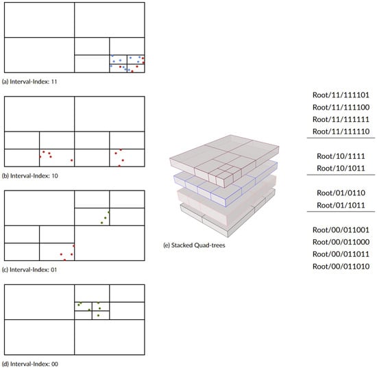
Figure 4.
Spatial and temporal location of the points in Figure 3. On the right side, the DSTree-Index related to each section of the graph is listed.
3.2. Insert
In order to insert a GI into a DSTree, a two-step process is required. First, we need to find the proper node on the interval tree part of the DSTree that can be added to. Afterward, we will add the to the proper quad-tree leaf using . To do so, we first obtain the low value of the interval at the root of DSTree. If the root’s low value is smaller than ’s low endpoint, then the new interval goes to the left sub-tree; otherwise, the new node goes to the right sub-tree. We continue the same process until the sub-tree level is equal to the temporal level (T) parameter of the DSTree. Once the node is selected, if there is already a quad-tree in the node (node is spatial), we insert the into the quad-tree using its parameter. If the node is empty, we generate a new quad-tree and proceed with adding it. Adding to the quad-tree is similar to the regular quad-tree insert (e.g., see [65]). Once all the steps are completed, we update the max value of the ancestors of interval tree portion if needed. Algorithm 1 shows the pseudocode for the process.
| Algorithm 1 Insert algorithm for the proposed DSTree |
| function insertGidIntoDSTree() |
| while is not a leaf do |
| if then |
| else |
| end if |
| end while |
| if is spatial then |
| insertIntoQuadTree() |
| else |
| newQuadTree |
| insertIntoQuadTree() |
| end if |
| updateAncestorsMaxValue() |
| end function |
| function insertIntoQuadTree() ▹ Perform regular quad-tree insert ▹ Implementation details depend on specific quad-tree algorithm ▹ See reference [65] |
| // Example steps: |
| // - Determine quadrant for |
| // - Recursively insert into appropriate quadrant of |
| end function |
| function updateAncestorsMaxValue() ▹ Check if max value of ancestors needs updating ▹ Traverse up the tree until root, updating max values as needed ▹ Implementation details depend on DSTree structure |
| end function |
Time Complexity of an Insert
The time complexity of inserting a into a DSTree involves several steps:
- Finding the proper node on the interval tree part of the DSTree: The time complexity of this operation depends on the height of the interval tree portion of the DSTree and the number of nodes visited during the traversal. In the worst case, if the interval tree portion is unbalanced, the time complexity can be , where n is the number of intervals in the DSTree.
- Adding the to the proper quad-tree leaf: Once the proper node on the interval tree part is found, adding the to the proper quad-tree leaf involves traversing the quad-tree structure. The time complexity of this operation depends on the size and structure of the quad-tree. In general, the time complexity of a quad-tree insertion can be , where m is the number of objects in the quad-tree.
- Updating the max value of the ancestors of the interval tree portion: After inserting the , the max value of the ancestors of the interval tree portion may need to be updated. The time complexity of this operation depends on the height of the interval tree portion of the DSTree. In the worst case, if the interval tree portion is unbalanced, the time complexity can be , where n is the number of intervals in the DSTree.
Overall, considering all steps, the time complexity of inserting a into a DSTree can be approximated as , where n is the number of intervals in the DSTree and m is the number of objects in the quad-tree. However, the actual time complexity may vary depending on the specific implementation details and the characteristics of the DSTree and quad-tree.
3.3. Delete
Deleting GI items from DSTree is a relatively complex process due to the complexities of removing intervals from a regular interval tree. After deleting a from the DSTree, if the node containing that contains no more objects, that node may be deleted from the tree. This involves promoting a node further from the leaf to the position of the node being deleted, which results in the reconstruction of the top part of the DSTree (for details about deleting items from interval trees, see [64], pp. 348–357). Algorithm 2 shows this process.
| Algorithm 2 Delete algorithm for the proposed DSTree |
| function deleteGidFromDSTree() |
| queryGidFromDstree() |
| if is found then |
| // remove the |
| if is empty after deletion then |
| // Delete the node from the tree |
| // Reconstruct the DSTree if necessary |
| end if |
| end if |
| end function |
| function queryGidFromDstree() ▹ Find the node which contains the current |
| end function |
Time Complexity of a Delete
The time complexity of deleting items from a DSTree involves several factors:
- Finding the node containing the : The time complexity of this operation depends on the structure of the DSTree. In the worst case, if the DSTree is unbalanced, the time complexity can be , where n is the number of nodes in the DSTree.
- Deleting the from the node: The time complexity of deleting the from the node depends on the data structure used to store intervals in the node. For interval trees, the deletion process can have a time complexity of , where i is the number of intervals in the node.
- Deleting the node from the DSTree if it contains no more objects: If the node contains no more objects after deleting the , it may need to be deleted from the tree. Deleting a node from a tree can involve restructuring the tree, which can have a time complexity of , where n is the number of nodes in the tree.
Overall, the time complexity of deleting items from a DSTree can be approximated as , where n is the number of nodes in the DSTree and i is number of intervals. However, the actual time complexity may vary depending on the specific implementation details and the characteristics of the DSTree.
3.4. Query
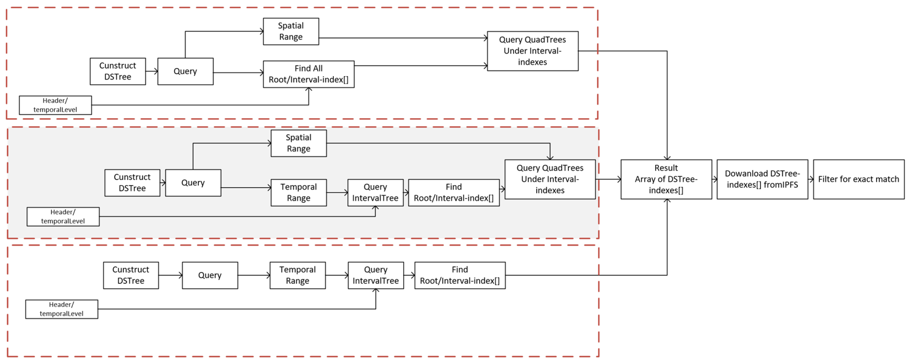
A spatio-temporal range search is a query of geographic objects that intersect with a boundary box, , in two-dimensional space and also is in a temporal topological relation, , with a time interval, [66]. There can be three main variations of queries of a DSTree, which include queries with both temporal interval and spatial extents, queries with only temporal interval, and queries with only spatial extent. Here, we only cover the first variation. The approach to those two variations is similar and explained in more detail in Figure 5. In order to perform a spatio-temporal range on a DSTree, it is required to first query the interval tree portion of the DSTree. If I is in relation with the root’s interval, we add the root’s interval to the candidate node list. If the left child of the root is not empty and the max value of the sub-tree in the left child is greater than I’s low value, recur for the left child; otherwise, recur for the right child. Once the candidate nodes are selected, if the selected nodes have a quad-tree as their sub-tree, we perform a quad-tree search for S; otherwise, we only check for the intersection of the selected node with the boundary box, S. Algorithm 3 shows this process.
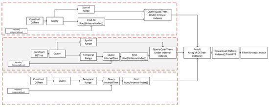
Figure 5.
Three main scenarios to process queries using DSTree. Top: When a user requests only a spatial range in which we search all the quad-trees in the DSTree. Middle: When the user queries spatial and temporal ranges together, DSTree first queries interval tree part of the graph and then searches quad-trees that exist at the bottom of those candidate nodes. Bottom: Cases where user only provides a temporal range. As a result, we only search interval tree part of the DSTree and then simply query the root of the quad-tree in each candidate node.
Time Complexity of a Query
The query process has three key operations, as follows:
- Querying the interval tree portion of the DSTree: This operation involves traversing the interval tree portion of the DSTree recursively. The time complexity of this operation depends on the height of the interval tree portion and the number of nodes visited during the traversal. If the interval tree portion is balanced, the time complexity is , where n is the number of intervals in the DSTree.
- Recursing down the left or right child nodes: This operation involves recursively traversing down the left or right child nodes of each candidate node. The time complexity of this operation depends on the structure of the DSTree and the distribution of intervals. In the worst case, if the DSTree is unbalanced, the time complexity can be , where i is the number of intervals in the DSTree.
- Quad-tree search: If the selected nodes have quad-tree sub-trees, a quad-tree search for S is performed. The time complexity of the quad-tree search depends on the size and structure of the quad-tree and the number of objects in the search area. In general, the time complexity of a quad-tree search is , where m is the number of objects in the search area and k is the number of objects found.
| Algorithm 3 Query algorithm for the proposed DSTree |
| function spatioTemporalRangeSearch() |
| empty list |
| queryIntervalTree() |
| if is not empty then |
| for each in do |
| if isIntervalInRelation() then |
| addToResult() |
| end if |
| if is not empty and |
| then |
| spatioTemporalRangeSearch() |
| else if is not empty then |
| spatioTemporalRangeSearch() |
| end if |
| end for |
| end if |
| for each in do |
| if then |
| quadTreeSearch() |
| else |
| if doesNodeIntersect() then |
| addToResult() |
| end if |
| end if |
| end for |
| end function |
| function queryIntervalTree() |
| if is null then |
| return |
| end if |
| if doesNodeIntersect() then |
| .append() |
| end if |
| queryIntervalTree() |
| queryIntervalTree() |
| end function |
Overall, considering all operations, the time complexity of the algorithm can be approximated as , where i is the number of intervals in the DSTree, m is the number of objects in the search area, and k is the number of objects found during the search.
3.5. Dstree Construction from Bulk Data
Since DSTree is a two-level tree, the performance of the insert, delete, and construction of the tree depends on both the top level and bottom level of the trees. Construction of the DSTree from scratch for bulk data is a relatively straightforward process. First of all, an interval tree is constructed based on the existing data. Once data are inserted into the hierarchical node structure, the algorithm traverses down from the root of the interval tree until the tree level equals the temporal level (T). Once the appropriate level is detected in the interval tree, all of the items under sub-trees (left and right branched) of the selected node are collected into one single node and a quad-tree is constructed in that node.
4. Performance Metrics
The behavior of the proposed tree structure is measured using a number of experiments with real data. These experiments are intended to reflect the conditions of common tasks involved in spatial and temporal queries of the data. Results of multiple models are compared to the method proposed. In the first set of the experiments, data on the occurrence of crime from the Waterloo Regional Police Service (https://www.wrps.on.ca/en/about-us/reports-publications-and-surveys.aspx, accessed on 15 February 2024) are used. These data detail all the police-reported occurrences for the calendar year. The time frame of these data is from 2017 to 2022. The data include occurrence data and time, response time, and geographic coordinates of the occurrence. In this experiment, only the location of each event and the response time of each event are used. In order to have a comparison between DSTree and the other existing models, we have used three other methods to process spatio-temporal queries. In choosing each method, the availability of source code to perform the tests was considered. Oct-tree is one of the methods which is used in the experiments similar to the work carried out by [47,52,53], in which the third dimension of cuboid data is considered as the time interval (source code available at [67]). The second access method used is a regular quad-tree (source code available at [68]). In this method, only a spatial query is performed, and then, to obtain the exact result set, all the results from the spatial query are tested to filter based on the temporal parameters. The third method is an interval tree (source code available at [69]). In this method, in contrast to the quad-tree method, only a temporal query is performed, and once the results are extracted from the tree structure, the spatial filter is applied to them to obtain the exact results. The above experiment is applied to the batches of 50 k, 100 k, 200 k, 400 k, 800 k, and 1 million points. Each test was executed five times then repeated ten times, and the average time of the execution was measured. The spatio-temporal query was constant over the entire experiment. The main query for these different models is defined as follows:
Find the events where their location has an topology relation with an extent equal to
and their response time has a topological relation T with a temporal extent of
where are the spatial extent of the entire dataset and are temporal extent of the data and T is the temporal topology from Table 1.
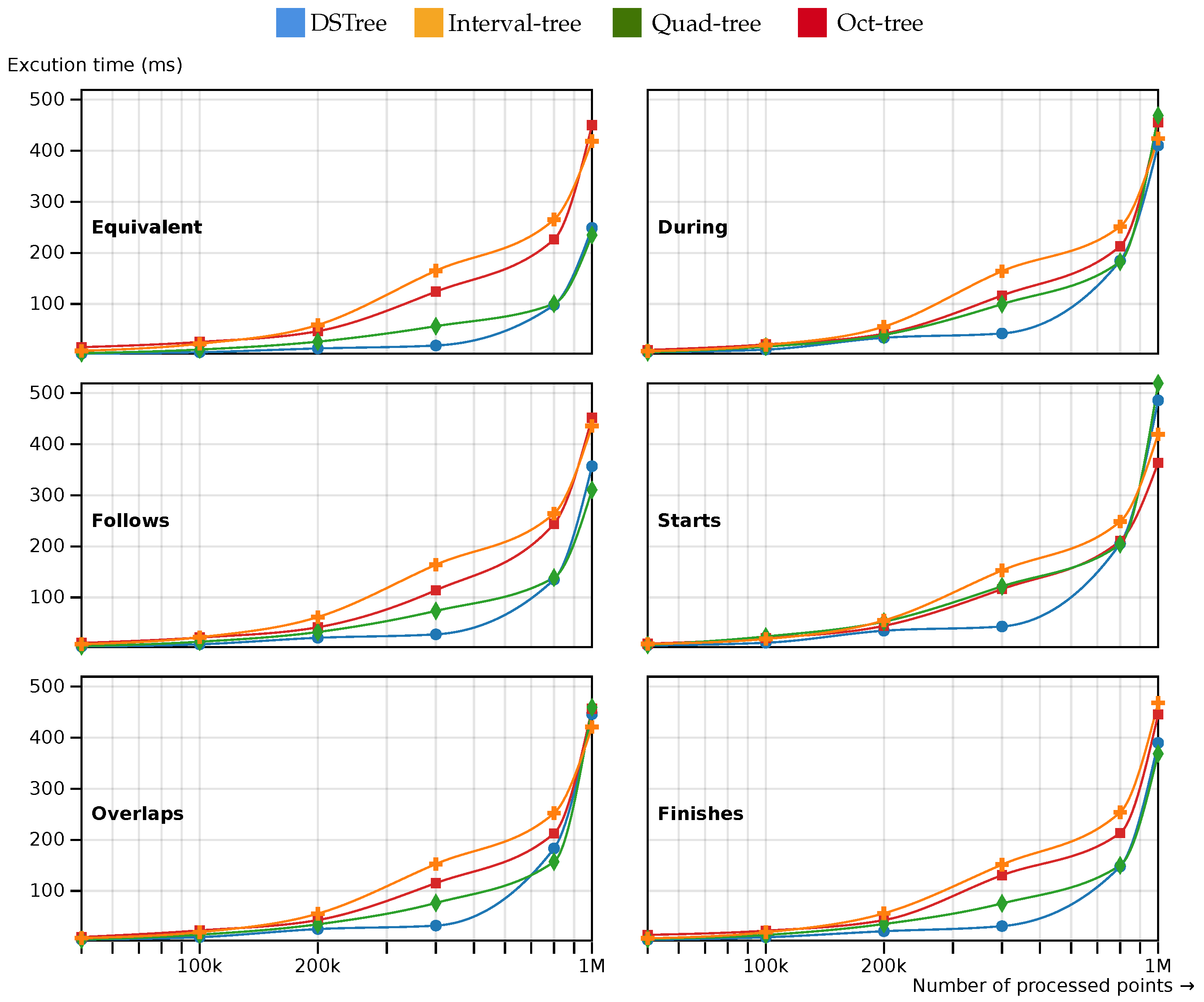
In Figure 6, the results of the six temporal queries are discussed. In these six queries, static spatial extent is used. As Figure 6 shows, DSTree shows a good performance for query processing in medium-sized datasets compared to other types of indexing methods. The metrics of the DSTrees in all of the six temporal topologies are close to the quad-tree method. Oct-tree and interval tree also show close performance metrics.
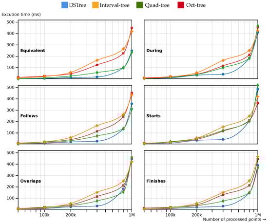
Figure 6.
The query processing time for different spatio-temporal access methods. The spatial and temporal extent of each query remained constant. The results are measured for 6 different temporal topologies.
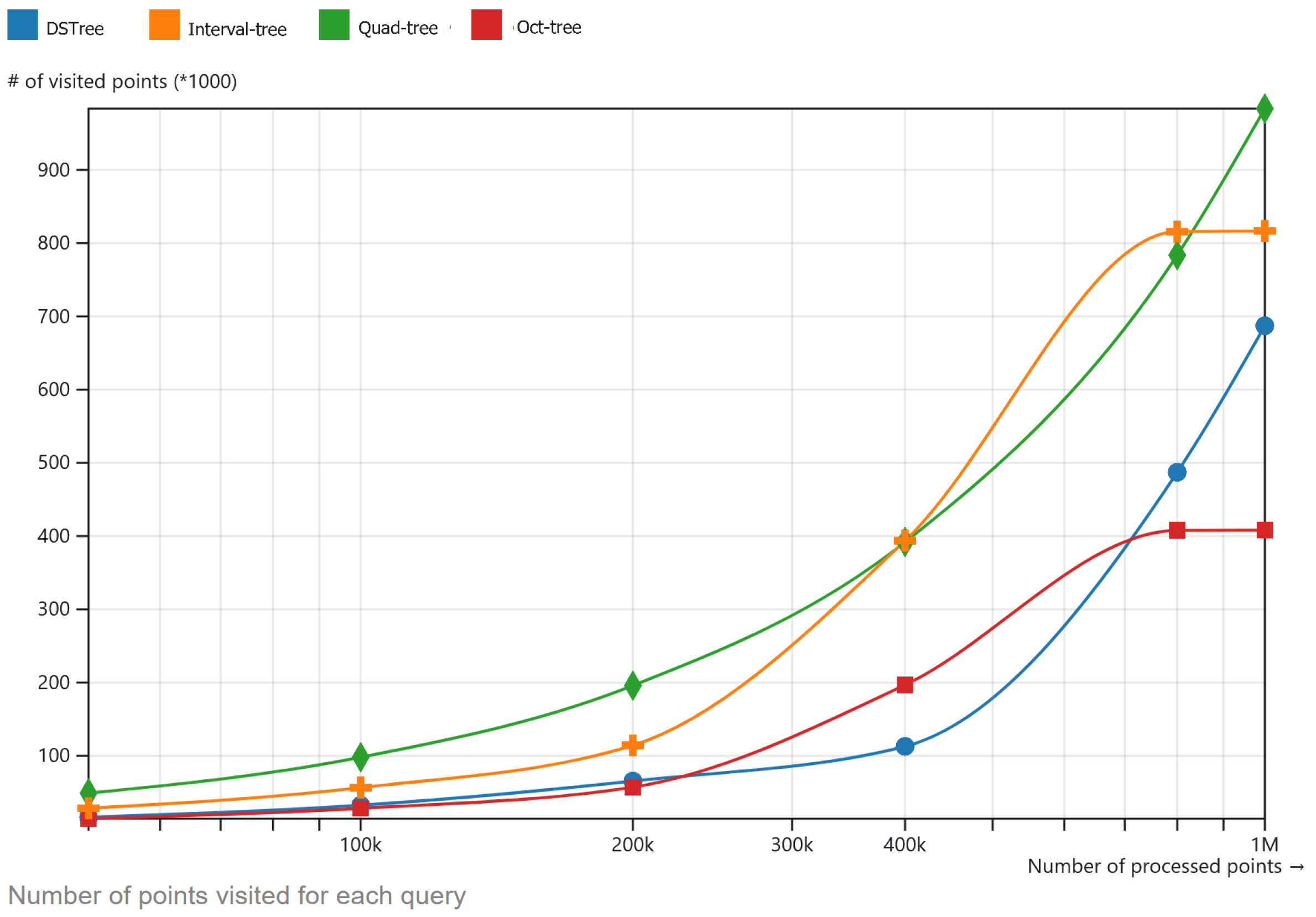
The second experiment is with the number of visited points in order to answer a constant spatio-temporal query. In the experiment, only objects that the index traverses and are checked to answer each query are counted. Figure 7 shows the results of this experiment. In this figure, DSTree has fewer visited points compared to quad-tree. The reason why they have close metrics is that the quad-tree is less computationally heavy compared to DSTree. As Figure 7 shows, the DSTree has visited less points than oct-tree and oct-tree suddenly flattened out after 800k points. This is probably related to the spatial distribution of the points on the area which are clustered and results in a better performance of oct-tree. Further studies are required to address this kind of edge case. However, considering this number of visited points, the time to create an oct-tree is 20% higher, which is discussed in the next section. In addition, since the oct-tree uses functions which involve the third dimension comparison, the query performance does not out-perform DSTree overall.

Figure 7.
Number of visited points in each model to answer a spatio-temporal query.
5. Ipfs
The first generation of P2P systems, namely file-sharing applications such as BitTorrent, support only keyword lookups and mostly provide no load balancing. The second generation is mainly structured P2P systems supporting basic key-based routing [31]. The InterPlanetary File System (IPFS) is a protocol and a P2P network for storing and sharing data in a distributed file system. IPFS uses content addressing to uniquely identify each file in a global namespace connecting all computing devices [70]. Each file on the IPFS network has a unique hash address which is used as a reference to request it from the network. Any user in the network can serve a file by its content address, and other peers in the network can find and request that content from any node that has it using a distributed hash table (DHT) [71].
At its core, IPFS is built on top of a data structure called InterPlanetary Linked Data (IPLD) [70]. The IPLD model is a set of specifications in support of decentralized data structures for the content-addressable web. Content IDs (CIDs) are hashes generated to allow the user to interact with IPFS in a trustless manner and recover their data. IPLD deals with decoding these hashes so that users can access their data. When new content is added to the IPFS network, that content is separated into several chunks and stored in different blocks. To reconstruct the whole file, a Directed Acyclic Graph (DAG) connects each bit of content together. In a DAG, we can only move from parent nodes to child nodes as each edge is oriented. Hierarchical data in particular are very naturally represented via DAGs.
IPLD creates a series of links to data internally but also allows users to create those links themselves through simple data structures that can be stored on IPFS. This capability allows us to store a DAG graph (in our case, a DSTree) on IPFS. This capability allows users to request a portion of the data from the network without the need to download the entire dataset. For example, a user is able to store a graph, shown in Figure 3, as an IPLD object, as shown in Table 2. IPLD’s capability to store and retrieve DAG graphs allows us to store spatio-temporal data as a graph structure, and as a result, we can request them based on the query parameters. DSTree only keeps a CID reference to the actual feature in each tree leaf. So depending on the query parameters, we only need to retrieve a portion of the GI or specific subtree of the DSTree. In an IPLD, each graph node is separated using /. For example, a DSTree leaf can be represented as an IPLD hash as
where DSTreeCID is the CID of the root of the DSTree, Interval-treeindex is the interval tree portion, and quad-treeindex is the second portion of the DSTree index. Under each leaf, there will be a series of GI objects. Each GI can be stored separately on IPFS, and its own CID, GICID, can be used as a reference to the object itself. So to access a single feature, we can use an IPFS address similar to DSTreeCID/Interval-treeindex/quad-treeindex/GICID. Note that GICID is generated based on the content of the GI by IPFS, and to have access to it, we need to query it from DSTree.
Table 2.
An example of how IPFS stores a DAG graph (based on the graph in Figure 3) and how to request a portion of the graph from the IPFS. Qmb...R is DSTreeCID which is a hash generated based on the root content of entire DAG graph from the DSTree Qmb...d or Qmb...c is a GICID, which is a hash generated based on the content of single object.
6. Distributed Network Integration
In order to process queries on distributed networks (in our case IPFS), it is required to store data in a DAG format. We use DSTree to construct a DAG graph, and once the tree structure is constructed, an IPLD graph is formed from the DSTree graph. Then, the IPLD object is stored on the IPFS network and a CID of the uploaded contents is used as a root gateway to access the entire tree structure. DSTree in this system acts as the main index structure to perform and answer spatio-temporal queries. Since DSTree is an indexing structure, it does not store the actual GI. It only stores the CID of each individual GI as a reference to the object itself. This provides a lightweight graph that can be used by each client.
6.1. Data Management
As mentioned earlier, the DSTree only stores a CID reference to the actual GI. The GI can be in any format (e.g., geojson, topojson, or other feature-level standards). In constructing the DSTree, each GI is first uploaded on the IPFS as a regular file or IPLD object. Then, for each GI, we will then have a set of . This object is then inserted into a DSTree and the related DAG graph is then constructed. Once all the GI objects are added to the DSTree, the graph structure is converted to an IPLD object and is uploaded on the IPFS and the pair of will be shared between users.
6.2. Metadata
Metadata are usually defined as data about data [72]. In order to provide interoperability between different systems, it is required to include metadata objects within shared content. In the DSTree, is used to store information related to the dataset and can include general spatial metadata objects (e.g., see [73,74,75]). The following metadata keys (Table 3) are necessary in order to provide minimum interoperability when sharing information using DSTree on IPFS.
Table 3.
Necessary metadata objects required for sharing DSTree on IPFS.
6.3. Architecture and Implementation
The proposed method to process queries on IPFS networks consists of four main components. Figure 8 shows the flow of the communication between users on a distributed network in order to query, retrieve, and store GI. The start of the data sharing process on IPFS is with a user, , willing to share a GI, , on the network. Once the user uploads the GI content on IPFS, they use its CID, MBR, and time interval associated to it, , to construct a DSTree. In this step, the user is able to keep adding as many GI objects as they want to the DSTree. Once the construction of the DSTree is finished, the necessary metadata are also added to the data structure, and an IPLD object, , is constructed from DSTree’s DAG graph. The is then uploaded on the IPFS network and the related IPFS root hash, , and its metadata, , are retrieved from IPFS. Since the is generated by IPFS based on the content of the DAG graph, we need to share this CID with other users to be able to access the index. In order to share the IPFS hash with other users, a smart contract is used. This smart contract is responsible for keeping a history of hashes over time and providing the latest hash to the users at any time. In our example, a simple smart contract using Solidity is developed and deployed on the Ethereum test network. This smart contract is used in a web application in order to provide access to the latest version of hash and its metadata when a user visits the web application. Once the hash is added to the smart contract, it will be available to all the users who connect to this smart contract.
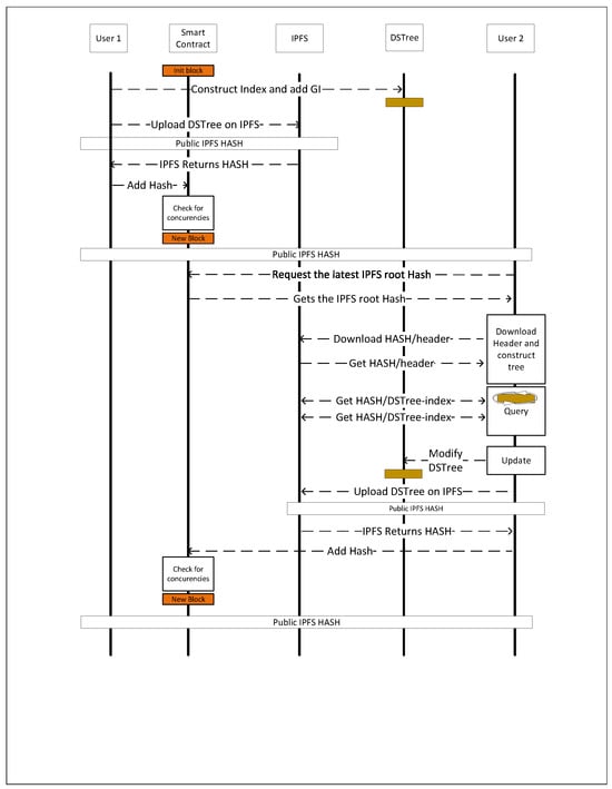
Figure 8.
Query process and publishing spatio-temporal data on the IPFS. It shows the process of sharing the DSTree index between users using a blockchain, querying the content from the network by another user, and updating the data on the network.
If a new user, , accesses the smart contract, then they will be able to fetch metadata and the IPLD DAG graph structure related to the DSTree. Then, they will be able to replicate a version of DSTree on their own local environment, and as a result, they are able to query data from that index. The results of the query, an array of s, are then requested from the IPFS through the query process explained in Figure 5.
If wants to add a new GI, , to the dataset, they first add it to the DSTree and then construct a new IPLD graph and upload the data on IPFS. Since the content of the new DSTree is different from the previous one, a new IPFS hash is generated and the is returned to the user. In the next step, connects to the smart contract and adds as a new block to the underlying blockchain. At this point, all the users will be able to access the updated data, , throughout the blockchain. The older version of the DSTree, , will also remain on the block history of the blockchain and will be accessible too.
7. Discussion
Unlike centralized systems, data storage in P2P networks is distributed across network nodes, providing scalability and no single point of failure. However, managing and processing queries on these networks has always been challenging. The proposed method to share and query spatio-temporal data on distributed networks tackles this issue by tracking and updating a spatio-temporal index between network users. In this approach, a blockchain is responsible for keeping a history of different versions of a DSTree index. Each user can replicate a version of DSTree on their node and run spatio-temporal queries on the index. Since each user performs the queries on their side, the indexing tree should check fewer items and support more topology out of the box. As shown in Figure 7, the number of visited items in the DSTree is generally less than other indexing structures, providing less memory consumption on the client apps. While octree also visits fewer nodes/items during its query process, its tree construction is slower (20%) compared to the other tree indexes. Also, it takes more time to answer the queries (see Figure 6) since the internal intersection functions are three-dimensional. They can also grow quickly if the time intervals are large [47]. In a single interval tree or quad-tree approach, the results of the queries need to be checked for the spatial or temporal topologies accordingly during the post-processing stage. In addition, the DSTree can handle six main temporal topological relations (see Table 1) during the query process without the need to post-process data. Time-wise, the DSTree also performs well on the small to average datasets (see Figure 6). Update, insertion, and deletion of existing data is another requirement for the current data-sharing environments. Due to using an interval tree as the top part of the tree, DSTree is not optimized for deleting items. Inserting a new GI will only update a portion of the tree structure and not impact the entire DAG data graph. However, adding data with large intervals so that the GI temporal interval covers branches from the left to the right side of the interval tree can cause a restructuring of the entire tree. For example, for time-series data such as sensor data or VGI, the DSTree performs better. In our police department example, the newly reported incidents can be added on top of the DSTree, and it does not cause the restructuring of the entire tree.
Conflicts may appear during the update process of the DSTree and publishing the latest version of DSTree by users. To resolve such conflicts, there are several approaches. Conflict resolution between different versions of DSTree can be achieved either on the client side before pushing the latest version on the blockchain or on the smart contract before saving . Both of these methods require a mechanism to detect and address conflicts. Because of the size limitations on the smart contracts, we are using a client-side conflict detection approach. In this approach, the DSTree graph is extracted from the latest version available on the blockchain and is compared with the version of the graph on the client side [76]. Supposing the conflicts in the DSTree graph are detected (using tools like [77]), the user will need to resolve the conflict and then publish it on the blockchain. However, this approach needs a trustful user interaction with the network.
The reason for using quad-trees is that since the root boundary box of all the quad-trees is constant, the quad index part of the DSTree index will always point to the same area in the geographic space over different time intervals. This provides a faster access method and the capability to exchange the quad-tree with a Discrete Global Grid System (DGGS). DGGS grid, similar to quad-tree, provides the same index value per each grid cell in the space. It also provides methods to aggregate data on multi-resolution levels [78,79,80] and also provides built-in data locality and directionality of space [81]. For instance, in sharing police department information over time, the reports can be censored using distributed k-anonymity methods on the P2P networks (e.g., [82]) if the DGGS system is used as feature data storage.
7.1. Data Locality in the IPFS with DSTree
Data locality implies that neighboring multidimensional information is stored in neighboring nodes [31]. In an IPFS network, once each node downloads some particular content, it can be a data provider. Combining data partitioning using DSTree and sharing data on IPFS at the GI level allows users to request only a small portion of the entire dataset. As a result, they can also serve small chunks of a large dataset. This can provide a data locality in the P2P network based on user activities, e.g., on VGI platforms. In our police data sharing example, once the dispatch teams share their location on the network, they have already become a data provider for that shared GI. Once the police officers visit that location, once again, they download that GI, and they will become another data provider for that specific GI on the IPFS network. This approach provides a level of data locality for the nodes close to each other since the nodes in a region usually tend to explore data related to their region. Other examples of use cases of such data locality include sharing geo-tagged information in small communities.
7.2. DSTree Limitations
The proposed DSTree model only supports the spatial topologies that the underlying spatial indexing method supports. In this paper, we only experimented with the intersection topology relation. However, it is possible to perform other topological relations such as overlay, within, and crosses and also perform KNN-based models. All of the temporal typologies are supported except disjoint. The focus of this paper was support for vector-based data structures. However, supporting raster data could be achieved by converting raster data into DGGS-based models or tiling the raster data instead of generating lower-level spatial index using the multi-resolution tiling structure. Table 4 summarizes supported queries and future approaches to support other data models.
Table 4.
DSTree capabilities for different spatio-temporal data models.
In this work, our focus was on spatio-temporal queries. However semantic queries play an important role in data retrieval. The potential of combining DSTree with models such as STKST-I [83] would allow querying semantic data, along with providing a wider range of temporal topologies.
8. Conclusions
P2P has become very popular decentralized approach for storing and sharing information. The daily amount of spatial data being collected and shared in different sectors with different levels highlights the need for P2P data management, query, and processing. This paper proposes a new spatio-temporal multi-level tree structure, DSTree, which aims to address this problem. DSTree is capable of performing a range of spatio-temporal queries. To integrate this data structure on the IPFS distributed network, a framework that uses blockchain to share the IPFS CID of the index is proposed. Each user is capable of replicating DSTree and querying or updating it. However, this model is not optimized for deletion and is mainly suitable for append-only data over time. In this work, some of the challenges in sharing and querying spatio-temporal data on distributed networks are addressed. Despite the advantages of our proposed framework, challenges remain. We conclude that more significant research effort from GIScience and related fields in developing decentralized applications is needed. The need for the standardization of different feature types and feature type properties when sharing data on the IPFS network is one of the requirements. The possibility of using IPLD objects in sharing GI at the feature level can provide finer access to the information. In addition, it is necessary to address attribute-level query processing, which is not covered in the current work. The use of the smart contract to control access of the users to read and write data to the main chain can also be studied. This access control can even be at the feature level.
Author Contributions
Conceptualization, M.H. and S.R.; methodology, M.H. and C.R.; software, M.H.; writing—original draft preparation, M.H.; writing—review and editing, S.R.; supervision, S.R. and C.R. All authors have read and agreed to the published version of the manuscript.
Funding
This research was funded by Global Water Future grant.
Data Availability Statement
The test dataset for the occurrence of the crime from the Waterloo Regional Police Service is available at (https://www.wrps.on.ca/en/about-us/reports-publications-and-surveys.aspx, accessed on 15 February 2024). Other data used in this paper are available upon request from the corresponding author. The prototype application, screenshots, and the source code for the app and its online version are available on GitHub at https://github.com/am2222/dstree, accessed on 15 February 2024.
Acknowledgments
The authors thank the Global Water Futures research program for funding this work under the Developing Big Data and Decision Support Systems theme.
Conflicts of Interest
The authors declare no conflicts of interest.
Abbreviations
The following abbreviations are used in this manuscript:
| IPFS | Interplanetary File System |
| DSTree | Distributed Spatio-temporal Tree |
| DHT | Distributed Hash Tree |
| P2P | Peer-to-Peer |
| KNN | K-nearest neighbor |
| DGGS | Discrete global grid system |
| DAG | Directed acyclic graph |
| IPLD | InterPlanetary Linked Data |
| CID | Content ID |
| GI | Geographic information |
References
- Goodchild, M.F.; Fu, P.; Rich, P. Sharing Geographic Information: An Assessment of the Geospatial One-Stop. Ann. Assoc. Am. Geogr. 2007, 97, 250–266. [Google Scholar] [CrossRef]
- Anderson, J. OpenStreetMap Contributor LifeSpans—Revisiting and Expanding on 2018 Research Paper. Available online: https://www.openstreetmap.org/user/Jennings%20Anderson/diary/398034 (accessed on 15 February 2024).
- Doulkeridis, C.; Vlachou, A.; Nørvåg, K.; Kotidis, Y.; Vazirgiannis, M. Efficient search based on content similarity over self-organizing P2P networks. Peer Peer Netw. Appl. 2010, 3, 67–79. [Google Scholar] [CrossRef]
- Al-Yadumi, S.; Xion, T.E.; Wei, S.G.W.; Boursier, P. Review on integrating geospatial big datasets and open research issues. IEEE Access 2021, 9, 10604–10620. [Google Scholar] [CrossRef]
- Group, T.H. Hierarchical Data Format (HDF). 2023. Available online: https://www.hdfgroup.org/ (accessed on 15 February 2024).
- Mahecha, M.D.; Gans, F.; Brandt, G.; Christiansen, R.; Cornell, S.E.; Fomferra, N.; Kraemer, G.; Peters, J.; Bodesheim, P.; Camps-Valls, G.; et al. Earth system data cubes unravel global multivariate dynamics. Earth Syst. Dyn. 2020, 11, 201–234. [Google Scholar] [CrossRef]
- Geoparquet. Available online: https://github.com/opengeospatial (accessed on 15 February 2024).
- Apache Iceberg—Apache Iceberg—Iceberg.apache.org. 2022. Available online: https://iceberg.apache.org/ (accessed on 15 February 2024).
- Goodchild, M.F. The future of digital earth. Ann. GIS 2012, 18, 93–98. [Google Scholar] [CrossRef]
- Yu, J.; Wu, J.; Sarwat, M. Geospark: A cluster computing framework for processing large-scale spatial data. In Proceedings of the 23rd SIGSPATIAL International Conference on Advances in Geographic Information Systems, Seattle, WA, USA, 3–6 November 2015; pp. 1–4. [Google Scholar]
- Eldawy, A.; Mokbel, M.F. Spatialhadoop: A mapreduce framework for spatial data. In Proceedings of the 2015 IEEE 31st International Conference on Data Engineering, Seoul, Republic of Korea, 13–17 April 2015; IEEE: Piscataway, NJ, USA, 2015; pp. 1352–1363. [Google Scholar]
- Bambacht, J.; Pouwelse, J. Web3: A Decentralized Societal Infrastructure for Identity, Trust, Money, and Data. arXiv 2022, arXiv:2203.00398. [Google Scholar]
- Nofer, M.; Gomber, P.; Hinz, O.; Schiereck, D. Blockchain. Bus. Inf. Syst. Eng. 2017, 59, 183–187. [Google Scholar] [CrossRef]
- Nakamoto, S. Bitcoin: A Peer-to-Peer Electronic Cash System. Available online: https://www.ussc.gov/sites/default/files/pdf/training/annual-national-training-seminar/2018/Emerging_Tech_Bitcoin_Crypto.pdf (accessed on 15 February 2024).
- Hojati, M.; Feick, R.; Roberts, S.; Farmer, C.; Robertson, C. Distributed spatial data sharing: A new model for data ownership and access control. J. Spat. Inf. Sci. 2023, 27. [Google Scholar] [CrossRef]
- Djellabi, B.; Amad, M.; Baadache, A. Handfan: A flexible peer-to-peer service discovery system for internet of things applications. J. King Saud-Univ.-Comput. Inf. Sci. 2022, 34, 7686–7698. [Google Scholar] [CrossRef]
- Ye, W.; Khan, A.I.; Kendall, E.A. Distributed network file storage for a serverless (P2P) network. In Proceedings of the 11th IEEE International Conference on Networks, ICON2003, Atlanta, GA, USA, 4–7 November 2003; IEEE: Piscataway, NJ, USA, 2004. [Google Scholar]
- Ehiagwina, F.O.; Iromini, N.A.; Olatinwo, I.S.; Raheem, K.; Mustapha, K. A State-of-the-Art Survey of Peer-to-Peer Networks: Research Directions, Applications and Challenges. J. Eng. Res. Sci. 2022, 1, 19–38. [Google Scholar] [CrossRef]
- Achir, M.; Abdelli, A.; Mokdad, L.; Benothman, J. Service discovery and selection in IoT: A survey and a taxonomy. J. Netw. Comput. Appl. 2022, 200, 103331. [Google Scholar] [CrossRef]
- Crainiceanu, A.; Linga, P.; Gehrke, J.; Shanmugasundaram, J. Querying Peer-to-Peer Networks Using P-Trees. In Proceedings of the 7th International Workshop on the Web and Databases: Colocated with ACM SIGMOD/PODS 2004, New York, NY, USA, 17–18 June 2004; pp. 25–30. [Google Scholar] [CrossRef]
- Ramabhadran, S.; Ratnasamy, S.; Hellerstein, J.M. Prefix Hash Tree An Indexing Data Structure over Distributed Hash Tables. In Proceedings of the PODC 2004 Conference, St. John’s, NL, Canada, 25–28 July 2004. [Google Scholar]
- Hassanzadeh-Nazarabadi, Y.; Taheri-Boshrooyeh, S.; Özkasap, Ö. DHT-based Edge and Fog Computing Systems: Infrastructures and Applications. In Proceedings of the IEEE INFOCOM 2022—IEEE Conference on Computer Communications Workshops (INFOCOM WKSHPS), Virtual, 2–5 May 2022; IEEE: Piscataway, NJ, USA, 2022; pp. 1–6. [Google Scholar]
- Harren, M.; Hellerstein, J.M.; Huebsch, R.; Loo, B.T.; Shenker, S.; Stoica, I. Complex queries in DHT-based peer-to-peer networks. In Peer-to-Peer Systems; Lecture Notes in Computer Science; Springer: Berlin/Heidelberg, Germany, 2002; pp. 242–250. [Google Scholar]
- Triantafillou, P.; Pitoura, T. Towards a unifying framework for complex query processing over structured peer-to-peer data networks. In Databases, Information Systems, and Peer-to-Peer Computing; Lecture Notes in Computer Science; Springer: Berlin/Heidelberg, Germany, 2004; pp. 169–183. [Google Scholar]
- Xia, J.; Yang, C.; Li, Q. Building a spatiotemporal index for earth observation big data. Int. J. Appl. Earth Obs. Geoinf. 2018, 73, 245–252. [Google Scholar] [CrossRef]
- Mokbel, M.F.; Ghanem, T.M.; Aref, W.G. Spatio-temporal access methods. IEEE Data Eng. Bull. 2003, 26, 40–49. [Google Scholar]
- Mondal, A.; Lifu, Y.; Kitsuregawa, M. P2PR-tree: An R-tree-based spatial index for peer-to-peer environments. In Current Trends in Database Technology—EDBT 2004 Workshops; Lecture Notes in Computer Science; Springer: Berlin/Heidelberg, Germany, 2004; pp. 516–525. [Google Scholar]
- Morton, G.M. A Computer Oriented Geodetic Data Base and a New Technique in File Sequencing. In International Business Machines; IBM Ltd.: Ottawa, ON, Canada, 1966. [Google Scholar]
- Stocia, I. Chord: A scalable peer-to-peer lookup service for internet applications. ACM Sigcomm Comput. Commun. Rev. 2001, 31, 149–160. [Google Scholar] [CrossRef]
- Sahin, O.D.; Antony, S.; Agrawal, D.; Abbadi, A.E. Probe: Multi-dimensional range queries in p2p networks. In Proceedings of the International Conference on Web Information Systems Engineering, New York, NY, USA, 20–22 November 2005; Springer: Berlin/Heidelberg, Germany, 2005; pp. 332–346. [Google Scholar]
- Liang, S. A new peer-to-peer-based interoperable spatial sensor web architecture. Int. Arch. Photogramm. Remote. Sens. Spat. Inf. Sci. 2008, XXXVII. Available online: https://citeseerx.ist.psu.edu/document?repid=rep1&type=pdf&doi=3baee6b2370bf3b2cb8f503aeb08cf73c097e77b (accessed on 15 February 2024).
- Zhang, C.; Krishnamurthy, A.; Wang, R.Y. Skipindex: Towards a Scalable Peer-to-Peer Index Service for High Dimensional Data. Available online: https://www.comp.nus.edu.sg/~cs6203/guidelines/topic3/multi-dimension/skipindex.pdf (accessed on 15 February 2024).
- Maymounkov, P.; Mazières, D. Kademlia: A Peer-to-Peer Information System Based on the XOR Metric. In Proceedings of the Peer-to-Peer Systems, Cambridge, MA, USA, 7–8 March 2002; pp. 53–65. [Google Scholar] [CrossRef]
- Kantere, V.; Skiadopoulos, S.; Sellis, T. Storing and indexing spatial data in P2P systems. IEEE Trans. Knowl. Data Eng. 2009, 21, 287–300. [Google Scholar] [CrossRef]
- Tang, C.; Xu, Z.; Dwarkadas, S. Peer-to-peer information retrieval using self-organizing semantic overlay networks. In Proceedings of the 2003 Conference on Applications, Technologies, Architectures, and Protocols for Computer Communications, Karlsruhe, Germany, 25–29 August 2003; pp. 175–186. [Google Scholar]
- Demirbas, M.; Ferhatosmanoglu, H. Peer-to-peer spatial queries in sensor networks. In Proceedings of the Third International Conference on Peer-to-Peer Computing (P2P2003), Linköping, Sweden, 1–3 September 2003; IEEE: Piscataway, NJ, USA, 2003; pp. 32–39. [Google Scholar]
- Cai, W.; Zhou, S.; Qian, W.; Xu, L.; Tan, K.L.; Zhou, A. C2: A new overlay network based on can and chord. Int. J. High Perform. Comput. Netw. 2005, 3, 248–261. [Google Scholar] [CrossRef]
- Soro, A.; Lai, C. Range-capable Distributed Hash Tables. In Proceedings of the 3rd ACM Workshop On Geographic Information Retrieval (GIR 2006), Seattle, WA, USA, 10 August 2006. [Google Scholar]
- Jagadish, H.; Ooi, B.C.; Vu, Q.H.; Zhang, R.; Zhou, A. VBI-Tree: A Peer-to-Peer Framework for Supporting Multi-Dimensional Indexing Schemes. In Proceedings of the 22nd International Conference on Data Engineering (ICDE’06), Atlanta, GA, USA, 3–7 April 2006; p. 34. [Google Scholar] [CrossRef]
- Ganesan, P.; Yang, B.; Garcia-Molina, H. One torus to rule them all: Multi-dimensional queries in p2p systems. In Proceedings of the 7th International Workshop on the Web and Databases: Colocated with ACM SIGMOD/PODS 2004, San Diego, CA, USA, 17–18 June 2004; pp. 19–24. [Google Scholar]
- Vlachou, A.; Doulkeridis, C.; Nørvåg, K.; Kotidis, Y. Peer-to-Peer Query Processing over Multidimensional Data; Springer: New York, NY, USA, 2012. [Google Scholar] [CrossRef]
- Dangermond, J.; Goodchild, M.F. Building geospatial infrastructure. Geo-Spat. Inf. Sci. 2019, 23, 1–9. [Google Scholar] [CrossRef]
- Gebbert, S.; Pebesma, E. A temporal GIS for field based environmental modeling. Environ. Model. Softw. 2014, 53, 1–12. [Google Scholar] [CrossRef]
- Yuan, M. Temporal GIS and spatio-temporal modeling. In Proceedings of the Third International Conference Workshop on Integrating GIS and Environment Modeling, Sante Fe, NM, USA, 21–25 January 1996; Volume 33. [Google Scholar]
- Pelekis, N.; Theodoulidis, B.; Kopanakis, I.; Theodoridis, Y. Literature review of spatio-temporal database models. Knowl. Eng. Rev. 2004, 19, 235–274. [Google Scholar] [CrossRef]
- Theodoridis, Y.; Vazirgiannis, M.; Sellis, T. Spatio-temporal indexing for large multimedia applications. In Proceedings of the Third IEEE International Conference on Multimedia Computing and Systems, Hiroshima, Japan, 17–23 June 1996; IEEE: Piscataway, NJ, USA, 1996. [Google Scholar] [CrossRef]
- Mahmood, A.R.; Punni, S.; Aref, W.G. Spatio-temporal access methods: A survey (2010–2017). Geoinformatica 2019, 23, 1–36. [Google Scholar] [CrossRef]
- He, Z.; Wu, C.; Liu, G.; Zheng, Z.; Tian, Y. Decomposition Tree: A Spatio-Temporal Indexing Method for Movement Big Data. Clust. Comput. 2015, 18, 1481–1492. [Google Scholar] [CrossRef]
- Armstrong, M.P. Temporality in spatial databases. In GIS/LIS 88 Proceedings: Accessing the World; Urban and Regional Information Systems Association: Des Plaines, IL, USA, 1988; pp. 880–889. [Google Scholar]
- Peuquet, D.J.; Duan, N. An event-based spatiotemporal data model (ESTDM) for temporal analysis of geographical data. Int. J. Geogr. Inf. Syst. 1995, 9, 7–24. [Google Scholar] [CrossRef]
- Jackins, C.L.; Tanimoto, S.L. Oct-trees and their use in representing three-dimensional objects. Comput. Graph. Image Process. 1980, 14, 249–270. [Google Scholar] [CrossRef]
- Zhang, C.; Zhu, L.; Long, J.; Lin, S.; Yang, Z.; Huang, W. A hybrid index model for efficient spatio-temporal search in HBase. In Lecture Notes in Computer Science; Springer International Publishing: Cham, Switzerland, 2018; pp. 108–120. [Google Scholar]
- Zhao, K.; Chen, L.; Cong, G. Topic Exploration in Spatio-Temporal Document Collections. In Proceedings of the 2016 International Conference on Management of Data, New York, NY, USA, 26 June–1 July 2016. [Google Scholar]
- Qu, Q.; Nurgaliev, I.; Muzammal, M.; Jensen, C.S.; Fan, J. On spatio-temporal blockchain query processing. Future Gener. Comput. Syst. 2019, 98, 208–218. [Google Scholar] [CrossRef]
- Zheng, Z.; Xie, S.; Dai, H.N.; Chen, X.; Wang, H. Blockchain challenges and opportunities: A survey. Int. J. Web Grid Serv. 2018, 14, 352–375. [Google Scholar] [CrossRef]
- PostGIS Clustering Data. Available online: https://postgis.net/workshops/postgis-intro/clusterindex.html (accessed on 15 February 2024).
- Liu, B.; Lee, W.C.; Lee, D.L. Supporting complex multi-dimensional queries in P2P systems. In Proceedings of the 25th IEEE International Conference on Distributed Computing Systems (ICDCS’05), Columbus, OH, USA, 6–10 June 2005; IEEE: Piscataway, NJ, USA, 2005. [Google Scholar]
- Allen, J.F. Maintaining knowledge about temporal intervals. In Readings in Qualitative Reasoning About Physical Systems; Elsevier: Amsterdam, The Netherlands, 1990; pp. 361–372. [Google Scholar]
- Gabbay, D.; Kurucz, A.; Wolter, F.; Zakharyaschev, M. Applied modal logic. In Many-Dimensional Modal Logics—Theory and Applications; Studies in logic and the foundations of mathematics; Elsevier: Amsterdam, The Netherlands, 2003; pp. 41–109. [Google Scholar]
- Qian, C.; Yi, C.; Cheng, C.; Pu, G.; Wei, X.; Zhang, H. Geosot-based spatiotemporal index of massive trajectory data. Isprs Int. J. Geo-Inf. 2019, 8, 284. [Google Scholar] [CrossRef]
- Sun, Y.; Zhao, T.; Yoon, S.; Lee, Y. A Hybrid Approach Combining R⁎-Tree and k-d Trees to Improve Linked Open Data Query Performance. Appl. Sci. 2021, 11, 2405. [Google Scholar] [CrossRef]
- Tao, Y.; Papadias, D. MV3R-Tree: A Spatio-Temporal Access Method for Timestamp and Interval Queries. In Proceedings of the 27th International Conference on Very Large Data Bases, San Francisco, CA, USA, 11–14 September 2001; pp. 431–440. [Google Scholar]
- de Berg, M.; Cheong, O.; van Kreveld, M.; Overmars, M. Computational Geometry, 3rd ed.; Springer: Berlin, Germany, 2008. [Google Scholar]
- Cormen, T.H.; Leiserson, C.E.; Rivest, R.L.; Stein, C. Introduction to Algorithms, 3rd ed.; The MIT Press: Cambridge, MA, USA, 2009. [Google Scholar]
- Finkel, R.A.; Bentley, J.L. Quad trees a data structure for retrieval on composite keys. Acta Inform. 1974, 4, 1–9. [Google Scholar] [CrossRef]
- Erwig, M.; Schneider, M. Developments in spatio-temporal query languages. In Proceedings of the Tenth International Workshop on Database and Expert Systems Applications, DEXA 99, Florence, Italy, 3 September 1999; IEEE: Piscataway, NJ, USA, 1999; pp. 441–449. [Google Scholar]
- d3-octree. Available online: https://github.com/vasturiano (accessed on 15 February 2024).
- quadtree-js. Available online: https://github.com/CorentinTh (accessed on 15 February 2024).
- flatten-interval-tree. Available online: https://github.com/alexbol99 (accessed on 15 February 2024).
- Benet, J. IPFS-Content Addressed, Versioned, P2P File System. arXiv 1974, arXiv:1407.3561. [Google Scholar]
- Zimmermann, R.; Ku, W.S.; Wang, H. Spatial data query support in peer-to-peer systems. In Proceedings of the 28th Annual International Computer Software and Applications Conference, COMPSAC 2004, Hong Kong, 28–30 September 2004; Volume 2, pp. 82–85. [Google Scholar] [CrossRef]
- Coulondre, S.; Libourel, T.; Spéry, L. Metadata And GIS: A Classification of Metadata for GIS. In Proceedings of the International Conference and Exhibition on Geographic Information, Lisbon, Portugal, 7–11 September 1998. [Google Scholar]
- Brodeur, J.; Coetzee, S.; Danko, D.; Garcia, S.; Hjelmager, J. Geographic information metadata—An outlook from the international standardization perspective. ISPRS Int. J. Geoinf. 2019, 8, 280. [Google Scholar] [CrossRef]
- Kim, T.J. Metadata for geo-Spatial data sharing: A comparative analysis. Ann. Reg. Sci. 1999, 33, 171–181. [Google Scholar] [CrossRef]
- Bossomaier, T.; Hope, B.A. Online GIS and Spatial Metadata, 2nd ed.; CRC Press: London, UK, 2015. [Google Scholar]
- Kleppmann, M.; Beresford, A.R. A Conflict-Free Replicated JSON Datatype. IEEE Trans. Parallel Distrib. Syst. 2017, 28, 2733–2746. [Google Scholar] [CrossRef]
- Automerge. Available online: https://github.com/automerge (accessed on 15 February 2024).
- Li, M.; Stefanakis, E. Geospatial operations of discrete global grid systems—A comparison with traditional GIS. J. Geovisualization Spat. Anal. 2020, 4, 26. [Google Scholar] [CrossRef]
- Robertson, C.; Chaudhuri, C.; Hojati, M.; Roberts, S.A. An integrated environmental analytics system (IDEAS) based on a DGGS. ISPRS J. Photogramm. Remote Sens. 2020, 162, 214–228. [Google Scholar] [CrossRef]
- Hojati, M.; Robertson, C.; Roberts, S.; Chaudhuri, C. GIScience research challenges for realizing discrete global grid systems as a Digital Earth. Big Earth Data 2022, 6, 358–379. [Google Scholar] [CrossRef]
- Sahr, K. Central place indexing: Hierarchical linear indexing systems for mixed-aperture hexagonal discrete global grid systems. Cartogr. Int. J. Geogr. Inf. Geovisualization 2019, 54, 16–29. [Google Scholar] [CrossRef]
- Hojati, M.; Farmer, C.; Feick, R.; Robertson, C. Decentralized geoprivacy: Leveraging social trust on the distributed web. Geogr. Inf. Syst. 2021, 35, 2540–2566. [Google Scholar] [CrossRef]
- Wu, X.; Liu, Y.; Zhao, X.; Chen, J. STKST-I: An Efficient Semantic Trajectory Search by Temporal and Semantic Keywords. Expert Syst. Appl. 2023, 225, 120064. [Google Scholar] [CrossRef]


Disclaimer/Publisher’s Note: The statements, opinions and data contained in all publications are solely those of the individual author(s) and contributor(s) and not of MDPI and/or the editor(s). MDPI and/or the editor(s) disclaim responsibility for any injury to people or property resulting from any ideas, methods, instructions or products referred to in the content. |
© 2024 by the authors. Licensee MDPI, Basel, Switzerland. This article is an open access article distributed under the terms and conditions of the Creative Commons Attribution (CC BY) license (https://creativecommons.org/licenses/by/4.0/).