
Partitioning Uncertainty in Model Predictions from Compartmental Modeling of Global Carbon Cycle

Abstract
:1. Introduction
2. Modeling Compartmental Systems
3. Models and Emission Scenarios
3.1. The Three GCC Models
3.1.1. Model I
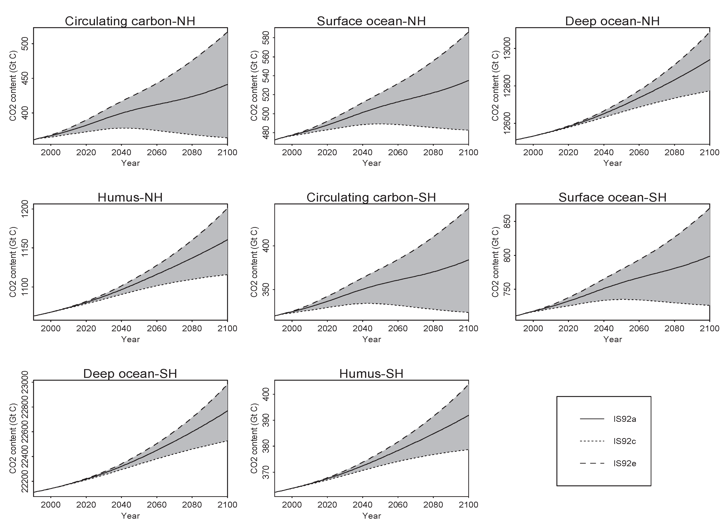
3.1.2. Model II
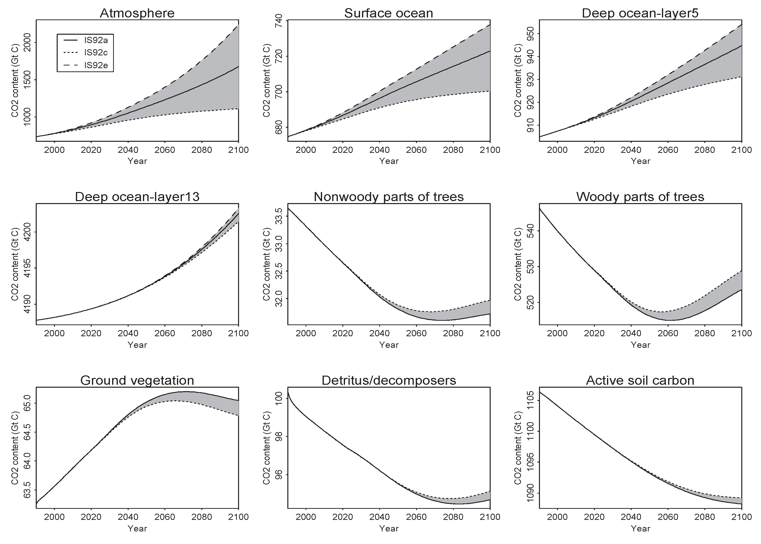
3.1.3. Model III
3.2. Emission Scenarios
4. Uncertainties in GCC Models
4.1. Main Sources of Uncertainty
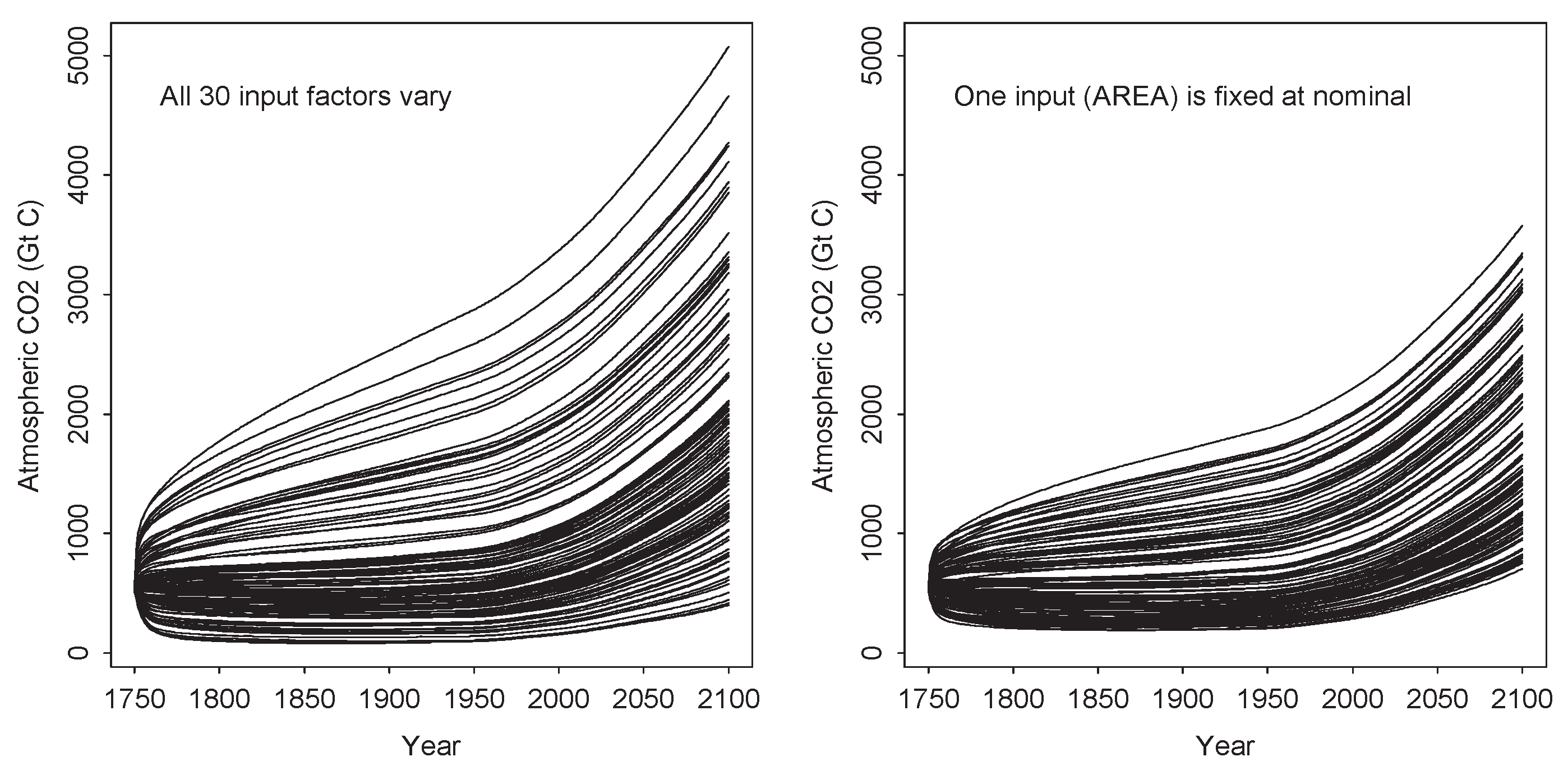
4.1.1. Input Factor Uncertainty
4.1.2. Scenario Uncertainty
4.1.3. Model Uncertainty
4.2. Delving Deeper into Primary Uncertainty Sources
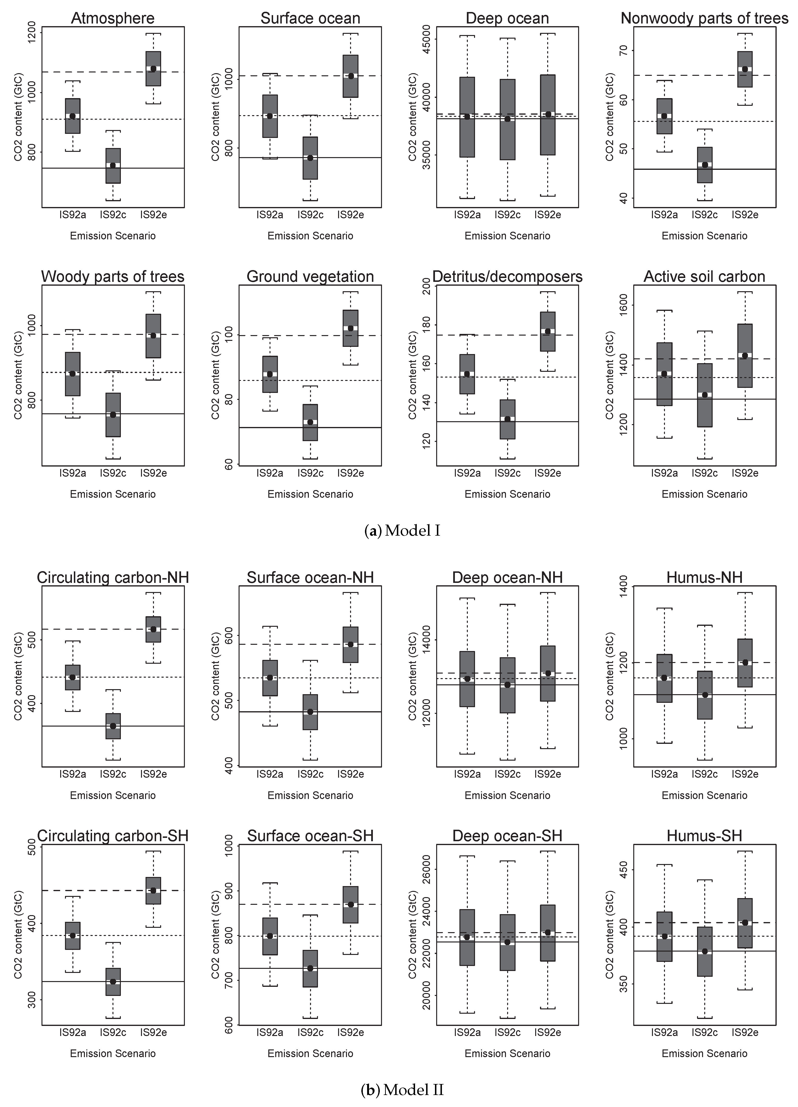
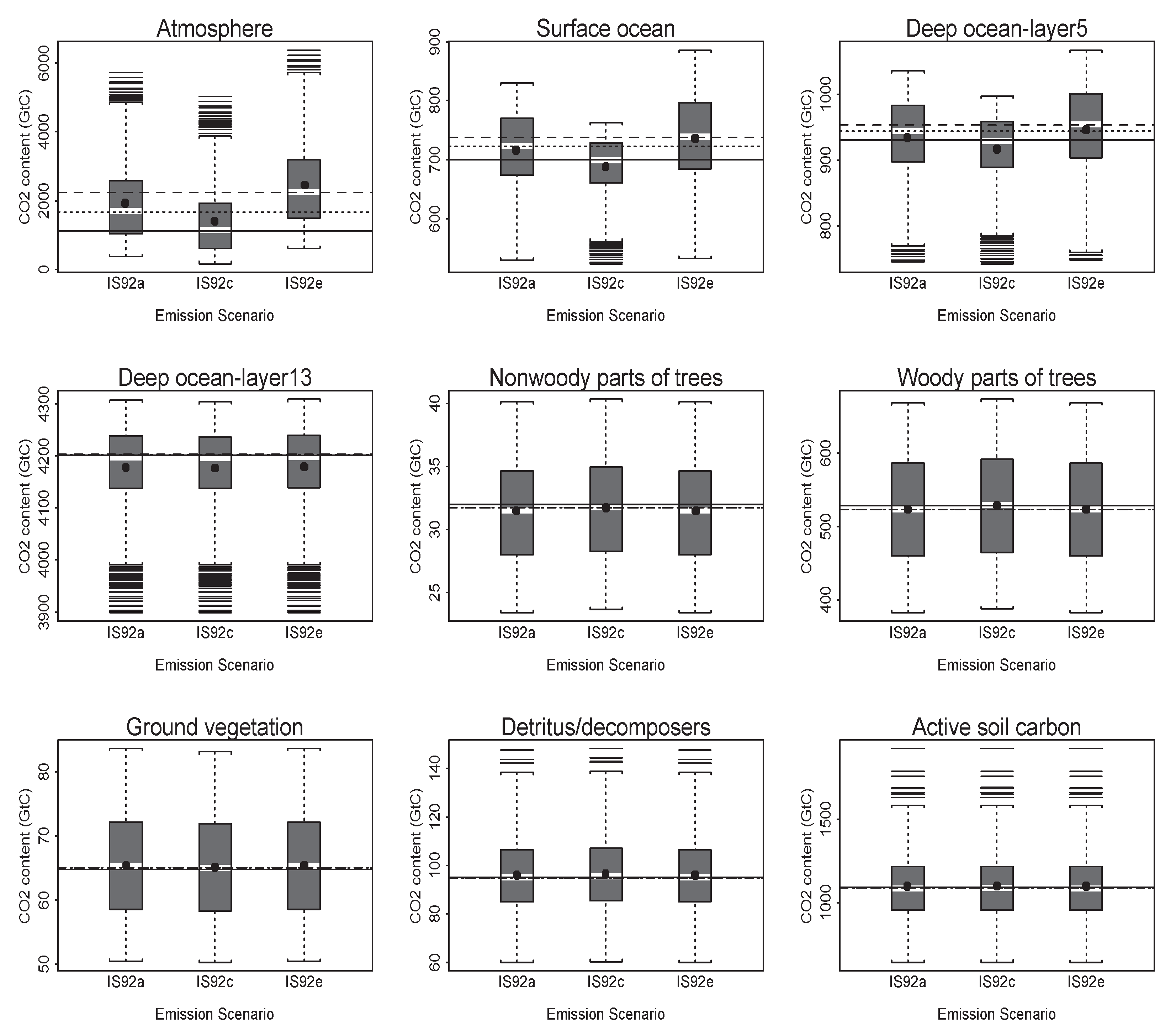
4.2.1. Input Factor Uncertainty within Models and Scenarios
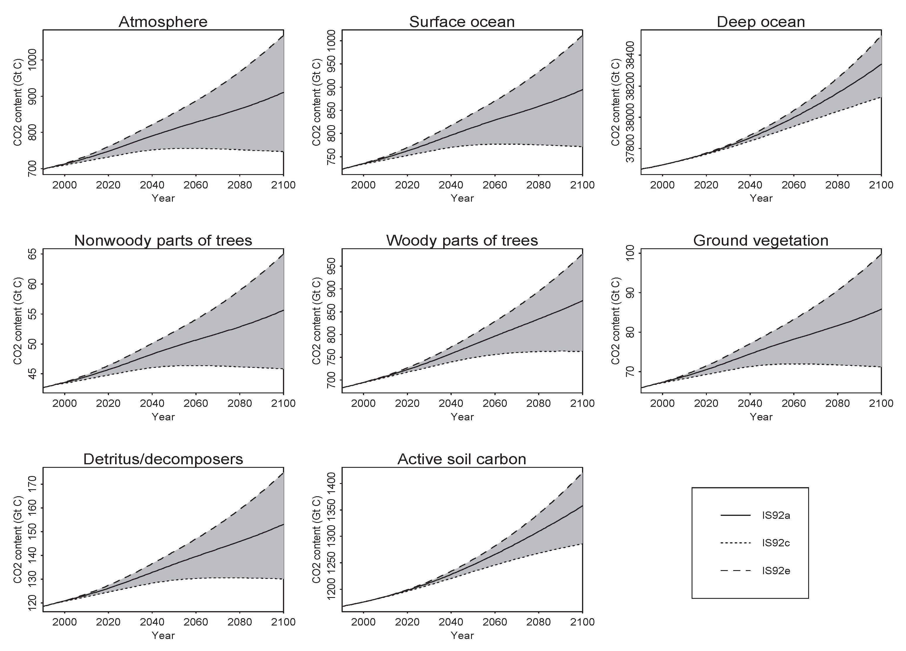
4.2.2. Scenario Uncertainty within Models
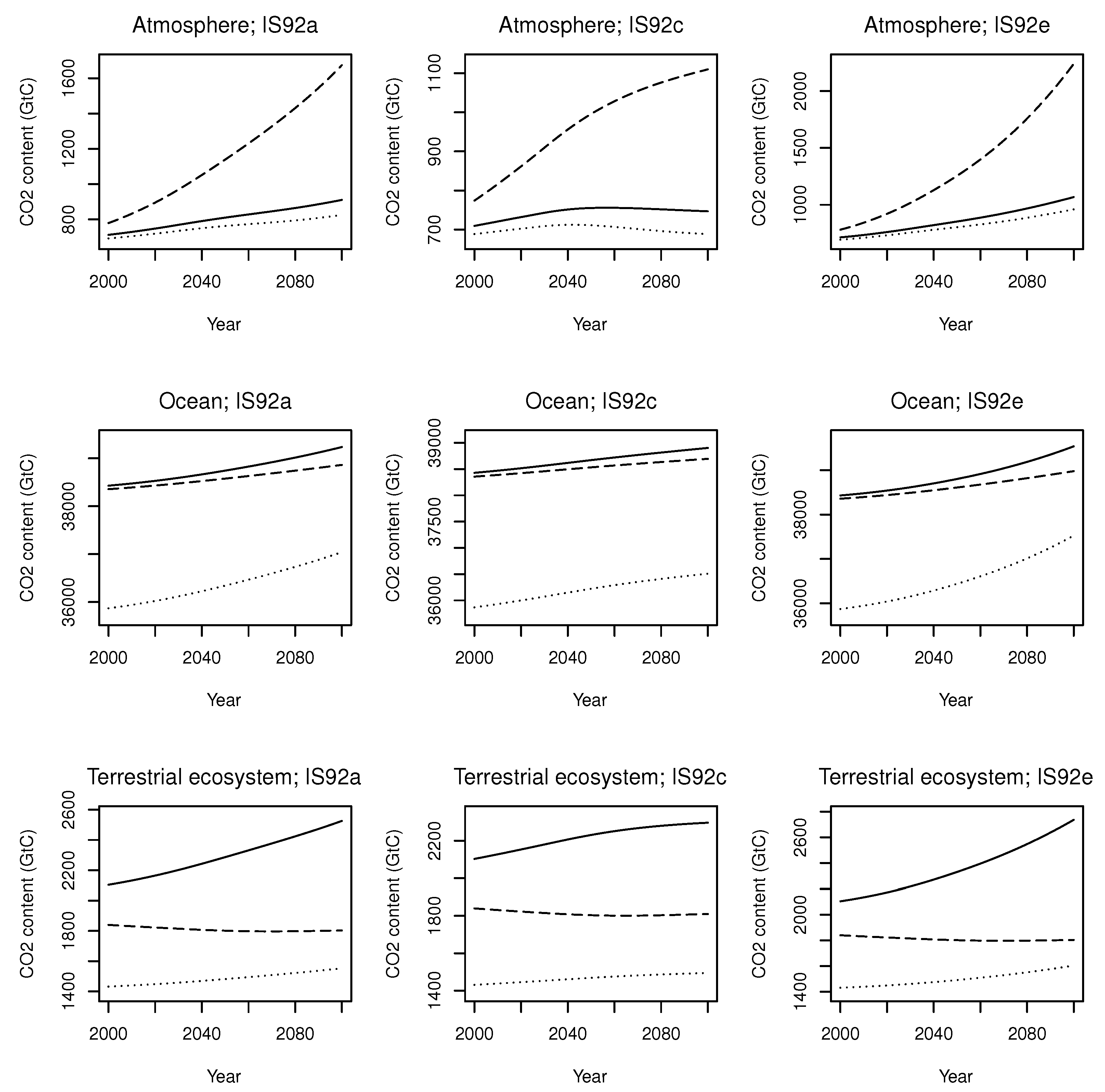
4.2.3. Model Uncertainty within Scenarios
5. Partitioning Uncertainty
6. Discussion
Funding
Data Availability Statement
Conflicts of Interest
References
- Perincherry, V.; Kikuchi, S.; Hamamatsu, Y. Uncertainties in the analysis of large-scale systems. In Uncertainty Modelling and Analysis: Theory and Applications—Machine Intelligence and Pattern Recognition Series; Ayyub, B.M., Gupta, M.M., Eds.; Elsevier Science Ltd.: Amsterdam, The Netherlands, 1994; Volume 17, pp. 73–96. [Google Scholar]
- Gazioğlu, S.; Scott, E.M. Sensitivity Analysis of Linear Time-Invariant Compartmental Models with Steady-State Constraint. J. Appl. Stat. 2011, 38, 2485–2509. [Google Scholar] [CrossRef]
- Cobelli, C.; Romanin-Jacur, G. Controllability, Observability and Structural Identifiability of Multi Input and Multi Output Biological Compartmental Systems. IEEE Trans. Biomed. Eng. 1976, BME-23, 93–100. [Google Scholar]
- Godfrey, K. Compartmental Models and Their Application; Academic Press: London, UK, 1983. [Google Scholar]
- Jacquez, J.A. Compartmental Analysis in Biology and Medicine, 2nd ed.; Michigan Press: Ann Arbor, MI, USA, 1985. [Google Scholar]
- Matis, J.H.; Wehrly, T.E. Stochastic Models of Compartmental Systems. Biometrics 1979, 35, 199–220. [Google Scholar] [CrossRef]
- Brown, R.F. Compartmental System Analysis: State of the Art. IEEE Trans. Biomed. Eng. 1980, BME-27, 1–11. [Google Scholar]
- Zierler, K. A Critique of Compartmental Analysis. Annu. Rev. Biophys. Bioeng. 1981, 10, 563–592. [Google Scholar] [CrossRef] [PubMed]
- Campolongo, F.; Saltelli, A. Sensitivity Analysis of an Environmental Model: An Application of Different Analysis Methods. Reliab. Eng. Syst. Saf. 1997, 57, 49–69. [Google Scholar] [CrossRef]
- Helton, J.C.; Johnson, J.D.; McKay, M.D.; Shiver, A.W.; Sprung, J.L. Robustness of an uncertainty and sensitivity analysis of early exposure results with the MACCS reactor accident consequence model. Reliab. Eng. Syst. Saf. 1995, 48, 129–148. [Google Scholar] [CrossRef]
- White, R.K. Evaluating the Reliability of Predictions Made Using Environmental Transfer Models; Safety Series No. 100; International Atomic Energy Agency: Vienna, Austria, 1989. [Google Scholar]
- Campolongo, F.; Tarantola, S.; Saltelli, A. Tackling Quantitatively Large Dimensionality Problems. Comput. Phys. Commun. 1999, 117, 75–85. [Google Scholar] [CrossRef]
- Helton, J.C.; Davis, F.J. Sampling-Based Methods for Uncertainty and Sensitivity Analysis; SAND99-2240; Sandia National Laboratories: Albuquerque, NM, USA, 2000.
- Helton, J.C.; Davis, F.J. Latin hypercube sampling and the propagation of uncertainty in analyses of complex systems. Reliab. Eng. Syst. Saf. 2003, 81, 23–69. [Google Scholar] [CrossRef]
- Emanuel, W.R.; Killough, G.G.; Post, W.M.; Shugart, H.H. Modeling terrestrial ecosystems in the global carbon cycle with shifts in carbon storage capacity by land-use change. Ecology 1984, 65, 970–983. [Google Scholar] [CrossRef]
- Kelly, G.N.; Jones, J.A.; Bryant, P.M.; Morley, F. The Predicted Radiation Exposure of the Population of the European Community Resulting from Discharges of Krypton-85, Tritium, Carbon-14 and Iodine-129 from the Nuclear Power Industry to the Year 2000; (V/2676/75); Commission of the European Communities: Luxembourg, 1975; Available online: http://aei.pitt.edu/50798/ (accessed on 5 February 2023).
- Bush, R.P.; Smith, G.M.; White, I.F. Carbon-14 Waste Management (No. EUR 8749 EN); Commission of the Economic Community: Brussels, Belgium; Luxembourg, 1984; pp. 79–119. [Google Scholar]
- McCartney, M. Global and Local Effects of 14C Discharges from the Nuclear Fuel Cycle. Ph.D. Thesis, University of Glasgow, Glasgow, UK, 1987. [Google Scholar]
- Gazioğlu, S. Application of Sensitivity and Uncertainty Analyses to Linear, Time-Invariant Compartmental Models. Ph.D. Thesis, University of Glasgow, Glasgow, UK, 2002. [Google Scholar]
- Emanuel, W.R.; Killough, G.G.; Post, W.M.; Shugart, H.H.; Stevenson, M.P. Computer Implementation of a Globally Averaged Model of the World Carbon Cycle; TR010, DOE/NBB-0062; US Department of Energy, Oak Ridge National Laboratory: Oak Ridge, TN, USA, 1984.
- Boden, T.A.; Marland, G.; Andres, R.J. Global, Regional, and National Fossil-Fuel CO2 Emissions (1751–2014) (V. 2017); Oak Ridge National Laboratory: Oak Ridge, TN, USA, 1999. Available online: https://data.ess-dive.lbl.gov/view/doi:10.3334/CDIAC/00001_V2017 (accessed on 8 March 2024).
- Houghton, J.T.; Callander, B.A.; Varney, S.K. Climate Change 1992; The Supplementary Report to the IPCC Scientific Assessment; International Panel on Climate Change, WMO/UNEP: Bracknell, UK, 1992. [Google Scholar]
- Young, P. Data-based mechanistic modelling, generalised sensitivity and dominant mode analysis. Comput. Phys. Commun. 1999, 117, 113–129. [Google Scholar] [CrossRef]
- Young, P. The data-based mechanistic approach to the modelling, forecasting and control of environmental systems. Annu. Rev. Control 2006, 30, 169–182. [Google Scholar] [CrossRef]
- Paladino, O.; Hodaifa, G.; Neviani, M.; Seyedsalehi, M.; Malvis, A. Modeling in environmental interfaces. In Advanced Low-Cost Separation Techniques in Interface Science; Kyzas, G.Z., Mitropoulos, A.C., Eds.; Elsevier Science Ltd.: Amsterdam, The Netherlands, 2019; Volume 30, pp. 241–282. [Google Scholar]
- Fatichi, S.; Pappas, C.; Zscheischler, J.; Leuzinger, S. Modelling carbon sources and sinks in terrestrial vegetation. New Phytologist 2018, 221, 652–668. [Google Scholar] [CrossRef] [PubMed]
- Fatichi, S.; Leuzinger, S.; Körner, C. Moving beyond photosynthesis: From carbon source to sink-driven vegetation modeling. New Phytol. 2014, 201, 1086–1095. [Google Scholar] [CrossRef] [PubMed]
- Piao, S.; Liu, Z.; Wang, T.; Peng, S.; Ciais, P.; Huang, M.; Ahlstrom, A.; Burkhart, J.F.; Chevallier, F.; Janssens, I.A.; et al. Weakening temperature control on the interannual variations of spring carbon uptake across northern lands. Nat. Clim. Change 2017, 7, 359–363. [Google Scholar] [CrossRef]
- Draper, D. Assessment and propagation of model uncertainty. J. R. Stat. Soc. 1995, 57-B, 45–97. [Google Scholar]
- Draper, D.; Pereira, A.; Prado, P.; Saltelli, A.; Cheal, R.; Eguilior, S.; Mendes, B.; Tarantola, S. Scenario and parametric uncertainty in GESAMAC: A methodological study in nuclear waste disposal risk assessment. Comput. Phys. Commun. 1999, 117, 142–155. [Google Scholar] [CrossRef]
- Chatfield, C. Model uncertainty, data mining and statistical inference. J. R. Stat. Soc.-Ser. A 1995, 158, 419–466. [Google Scholar] [CrossRef]
- Kennedy, M.C.; O’Hagan, A. Bayesian calibration of computer models. J. R. Stat. Soc.-Ser. B 2001, 63, 1–25. [Google Scholar] [CrossRef]
- King, A.W.; Sale, M.J. A Plan for Intermodel Comparison of Atmospheric CO2 Projections with Uncertainty Analysis; Carbon Dioxide Information Center: Oak Rid, TN, USA, 1990. [Google Scholar]
- IPCC. Special Report on Emissions Scenarios (SRES): A Special Report of Working Group III of the Intergovernmental Panel on Climate Change; Nakićenović, N., Swart, R., Eds.; Cambridge University Press: Cambridge, UK, 2000; 599p, Available online: https://www.ipcc.ch/site/assets/uploads/2018/03/emissions_scenarios-1.pdf (accessed on 27 May 2024).
- Van Vuuren, D.P.; Edmonds, J.; Kainuma, M.; Riahi, K.; Thomson, A.; Hibbard, K.; Hurtt, G.C.; Kram, T.; Krey, V.; Lamarque, J.F.; et al. The representative concentration pathways: An overview. Clim. Change 2011, 109, 5–31. [Google Scholar] [CrossRef]
- IPCC. Climate Change 2014: Synthesis Report. Contribution of Working Groups I, II and III to the Fifth Assessment Report of the Intergovernmental Panel on Climate Change; Core Writing Team, Pachauri, R.K., Meyer, L.A., Eds.; IPCC: Geneva, Switzerland, 2014; 151p, Available online: https://www.ipcc.ch/site/assets/uploads/2018/05/SYR_AR5_FINAL_full_wcover.pdf (accessed on 27 May 2024).
- O’Neill, B.C.; Kriegler, E.; Ebi, K.L.; Kemp-Benedict, E.; Riahi, K.; Rothman, D.S.; Van Ruijven, B.J.; Van Vuuren, D.P.; Birkmann, J.; Kok, K.; et al. The roads ahead: Narratives for shared socioeconomic pathways describing world futures in the 21st century. Glob. Environ. Change 2017, 42, 169–180. [Google Scholar] [CrossRef]
- IPCC. Summary for Policymakers. In Climate Change 2021: The Physical Science Basis. Contribution of Working Group I to the Sixth Assessment Report of the Intergovernmental Panel on Climate Change; Masson-Delmotte, V., Zhai, V.P., Pirani, A., Connors, S.L., Péan, C., Berger, S., Caud, N., Chen, Y., Goldfarb, L., Gomis, M.I., et al., Eds.; Cambridge University Press: Cambridge, UK; New York, NY, USA, 2021; pp. 3–32. Available online: https://www.ipcc.ch/report/ar6/wg1/downloads/report/IPCC_AR6_WGI_FrontMatter.pdf (accessed on 27 May 2024). [CrossRef]
- Lan, X.; Keeling, R.F. Trends in Atmospheric Carbon Dioxide-Mauna Loa CO2 Annual Mean Data; NOAA/GML (gml.noaa.gov/ccgg/trends/): Boulder, CO, USA; Scripps Institution of Oceanography: San Diego, CA, USA, 2023. Available online: https://gml.noaa.gov/webdata/ccgg/trends/co2/co2_annmean_mlo.txt (accessed on 30 March 2024).


| Description | Input Factor | Nominal Value | Range | Unit | |
|---|---|---|---|---|---|
| Initial conditions | (1) Atmosphere | 622.40 | 497.92–746.88 | Gt C | |
| (2) Surface ocean | 667.37 | 533.90–800.84 | Gt C | ||
| (3) Deep ocean | 37,542.00 | 30,033.60–45,050.40 | Gt C | ||
| (4) Nonwoody parts of trees | 38.21 | 30.57–45.85 | Gt C | ||
| (5) Woody parts of trees | 634.47 | 507.58–761.36 | Gt C | ||
| (6) Ground vegetation | 59.32 | 47.46–71.18 | Gt C | ||
| (7) Detritus/decomposers | 108.22 | 86.58–129.86 | Gt C | ||
| (8) Active soil carbon | 1131.39 | 905.11–1357.67 | Gt C | ||
| Transfer Coefficients | Atmosphere → Surface Ocean | 0.1582 | 0.1266–0.1898 | ||
| Atmosphere → Nonwoody parts of trees | 0.0354 | 0.0283–0.0425 | |||
| Atmosphere → Woody parts of trees | 0.0408 | 0.0326–0.0490 | |||
| Atmosphere → Ground vegetation | 0.0241 | 0.0193 –0.0289 | |||
| Surface ocean → Atmosphere | 0.1476 | 0.1181–0.1771 | |||
| Surface Ocean → Deep ocean | 0.0473 | 0.0378–0.0568 | |||
| Deep ocean → Surface ocean | 0.0008 | 0.0006–0.0010 | |||
| Nonwoody parts of trees → Detritus/decomposers | 0.5758 | 0.4606–0.6910 | |||
| Woody parts of trees → Detritus/decomposers | 0.0353 | 0.0282–0.0424 | |||
| Woody parts of trees → Active soil carbon | 0.0047 | 0.0038–0.0056 | |||
| Ground vegetation → Detritus/decomposers | 0.1667 | 0.1334–0.2000 | |||
| Ground vegetation → Active soil carbon | 0.0862 | 0.0690–0.1034 | |||
| Detritus/decomposers → Atmosphere | 0.4688 | 0.3750–0.5626 | |||
| Detritus/decomposers → Active soil carbon | 0.0328 | 0.0262–0.0394 | |||
| Active soil carbon → Atmosphere | 0.0103 | 0.0082–0.0124 |
| Description | Input Factor | Nominal Value | Range | Unit | |
|---|---|---|---|---|---|
| Initial conditions | Circulating carbon (NH) 1 | 325.21 | 260.17–390.25 | Gt C | |
| Surface ocean (NH) | 448.31 | 358.65–537.97 | Gt C | ||
| Deep ocean (NH) | 12,426.00 | 9940.80–14,911.20 | Gt C | ||
| Humus (NH) | 1042.30 | 833.84–1250.76 | Gt C | ||
| Circulating carbon (SH) 2 | 291.59 | 233.27–349.91 | Gt C | ||
| Surface ocean (SH) | 677.54 | 542.03–813.05 | Gt C | ||
| Deep ocean (SH) | 21,983.00 | 17,586.40–26,379.60 | Gt C | ||
| Humus (SH) | 356.21 | 284.97–427.45 | Gt C | ||
| Transfer Coefficients | Circulating carbon (NH) → Surface Ocean (NH) | 0.1400 | 0.1120–0.1680 | ||
| Circulating carbon (NH) → Humus (NH) | 0.0160 | 0.0128–0.0192 | |||
| Circulating carbon (NH) → Circulating carbon (SH) | 0.5000 | 0.4000–0.6000 | |||
| Surface ocean (NH) → Circulating carbon (NH) | 0.1000 | 0.0800–0.1200 | |||
| Surface ocean (NH) → Deep ocean (NH) | 0.0900 | 0.0720–0.1080 | |||
| Surface ocean (NH) → Surface ocean (SH) | 0.1000 | 0.0800–0.1200 | |||
| Deep ocean (NH) → Surface ocean (NH) | 0.0032 | 0.0026–0.0038 | |||
| Deep ocean (NH) → Deep ocean (SH) | 0.0050 | 0.0040–0.0060 | |||
| Humus (NH) → Circulating carbon (NH) | 0.0050 | 0.0040–0.0060 | |||
| Circulating carbon (SH) → Circulating carbon (NH) | 0.5600 | 0.4480–0.6720 | |||
| Circulating carbon (SH) → Surface ocean (SH) | 0.2300 | 0.1840–0.2760 | |||
| Circulating carbon (SH) → Humus (SH) | 0.0061 | 0.0049–0.0073 | |||
| Surface ocean (SH) → Surface ocean (NH) | 0.0660 | 0.0528–0.0792 | |||
| Surface ocean (SH) → Circulating carbon (SH) | 0.1000 | 0.0800–0.1200 | |||
| Surface ocean (SH) → Deep ocean (SH) | 0.0900 | 0.0720–0.1080 | |||
| Deep ocean (SH) → Deep ocean (NH) | 0.0028 | 0.0022–0.0034 | |||
| Deep ocean (SH) → Surface ocean (SH) | 0.0028 | 0.0022–0.0034 | |||
| Humus (SH) → Circulating carbon (SH) | 0.0050 | 0.0040–0.0060 |
| Description | Input Factor | Nominal Value | Range | Unit |
|---|---|---|---|---|
| Initial conditions: | ||||
| Atmosphere () | CA0 | 548.80 | 510.7–596.0 | Gt C |
| Nonwoody parts of trees () | CF0 | 38.20 | 30.0–46.0 | Gt C |
| Woody parts of trees () | CW0 | 634.50 | 507.0–762.0 | Gt C |
| Ground vegetation () | CG0 | 59.30 | 47.0–72.0 | Gt C |
| Detritus/decomposers () | CD0 | 108.20 | 86.0–130.0 | Gt C |
| Active soil carbon () | CSL0 | 1131.00 | 905.0–1348.0 | Gt C |
| Forest clearing: | ||||
| Fraction of forest clearing carbon transferred to atmosphere () | PHIA | 0.5 | 0.4–0.6 | — |
| Fraction of forest clearing carbon transferred to detrit./decomp. () | PHID | 0.5 | 0.4–0.6 | — |
| Ratio of soil to detrit./decomp. flux to forest clearing flux () | PSIS | 0.1 | 0.08–0.12 | — |
| Fraction of forest clearing release that serves to decrease capacity for carbon storage in trees () | SXIT | 0.5 | 0.4–0.6 | — |
| Reforestation: | ||||
| Rate of re-establishment of tree compartments () | SIG | 1.0 × | 0.8 × –1.2 × | |
| Rate coefficient controlling the time required for trees to dominate ground vegetation () | SS | 0.2 | 0.16–0.24 | |
| Fraction of the change in capacity for carbon storage in trees that causes a change in capacity for storage in ground vegetation () | EPS | 0.5 | 0.4–0.6 | — |
| Physical and Chemical ocean: | ||||
| Depth of surface ocean | HM | 75.0 | 60.0–90.0 | m |
| Area of surface ocean | AREA | 3.61 × | 2.88 × –4.33 × | |
| Temperature change in surface ocean as a result of doubling atm. carbon content () | DELTP | 3.0 | 1.5–4.5 | K |
| Total boron concentration in surface ocean () | SIGB | 4.1 × | 3.27 × –4.90 × | mol/L |
| Initial temperature of surface ocean () | TEMP0 | 292.75 | 290.75–294.75 | K |
| Chlorinity of surface water () | CL | 19.24 | 15.0–23.0 | |
| Relative humidity in atmosphere () | RELHUM | 0.75 | 0.6–0.9 | — |
| Terrestrial turnover times: | ||||
| Nonwoody parts of trees () | TF | 1.75 | 1.4–2.1 | year |
| Woody parts of trees () | TW | 25.00 | 20.0–30.0 | year |
| Ground vegetation () | TG | 4.00 | 3.2–4.8 | year |
| Detritus/decomposers () | TD | 2.00 | 1.6–2.4 | year |
| Active soil carbon () | TSL | 100.00 | 80.0–120.0 | year |
| Soil-forming fractions: | ||||
| Woody parts of trees () | THW | 0.1180 | 0.094–0.14 | — |
| Ground vegetation () | THG | 0.3330 | 0.26–0.40 | — |
| Detritus/decomposers () | THD | 0.0625 | 0.05–0.075 | — |
| Intrinsic recovery times: | ||||
| Nonwoody parts of trees () | TT2 | 20.0 | 16.0–24.0 | year |
| Ground vegetation () | TV2 | 4.0 | 3.2–4.8 | year |
| Compartment | IS92a | IS92c | IS92e | Scenario a Uncer. Range | Sce. and In. Factor b Uncer. Range | |
|---|---|---|---|---|---|---|
| Model I | Atmosphere | 746.7 | 910.51 | 1067.97 | 321.27 | 560.31 |
| Surface ocean | 771.80 | 894.42 | 1011.44 | 239.64 | 488.65 | |
| Deep ocean | 38,130.16 | 38,342.57 | 38,527.41 | 397.25 | 14,445.26 | |
| N.woody parts trees | 45.87 | 55.63 | 64.99 | 19.13 | 34.05 | |
| Woody parts trees | 763.19 | 874.18 | 976.54 | 213.35 | 449.04 | |
| Ground vegetation | 71.26 | 85.85 | 99.80 | 28.54 | 51.86 | |
| Detritus/decomposers | 130.09 | 153.10 | 174.80 | 44.71 | 86.12 | |
| Active soil carbon | 1285.88 | 1357.38 | 1420.06 | 134.19 | 561.41 | |
| Model II | Circulating carbon (NH) | 364.43 | 441.26 | 516.85 | 152.42 | 263.44 |
| Surface Ocean (NH) | 482.58 | 535.00 | 586.07 | 103.49 | 256.56 | |
| Deep ocean (NH) | 12,773.49 | 12,940.26 | 13,087.97 | 314.49 | 4557.71 | |
| Humus (NH) | 1115.79 | 1160.47 | 1200.78 | 84.99 | 440.27 | |
| Circulating carbon (SH) | 323.85 | 384.00 | 443.10 | 119.25 | 218.80 | |
| Surface Ocean (SH) | 726.43 | 798.86 | 869.32 | 142.90 | 374.23 | |
| Deep ocean (SH) | 22,526.45 | 22,768.65 | 22,981.94 | 455.49 | 7961.98 | |
| Humus (SH) | 378.71 | 391.91 | 403.76 | 25.04 | 146.50 | |
| Model III | Atmosphere | 1109.99 | 1674.90 | 2238.98 | 1128.99 | 6212.12 |
| Surface ocean | 700.44 | 723.01 | 737.92 | 37.48 | 361.94 | |
| Deep ocean—layer5 | 931.13 | 944.70 | 953.98 | 22.85 | 324.50 | |
| Deep ocean—layer13 | 4201.45 | 4202.53 | 4203.30 | 1.85 | 410.52 | |
| N.woody parts trees | 31.97 | 31.72 | 31.72 | 0.25 | 16.96 | |
| Woody parts trees | 528.82 | 523.55 | 523.55 | 5.28 | 291.39 | |
| Ground vegetation | 64.79 | 65.05 | 65.05 | 0.26 | 33.40 | |
| Detritus/decomposers | 95.13 | 94.68 | 94.68 | 0.46 | 88.48 | |
| Active soil carbon | 1089.23 | 1088.24 | 1088.24 | 0.99 | 1283.69 |
| Model Component | Model I | Model II | Model III | ||||
|---|---|---|---|---|---|---|---|
| Mean | CV | Mean | CV | Mean | CV | ||
| IS92a | Atmosphere | 920.89 | 7.29 | 825.25 | 5.86 | 1926.86 | 57.69 |
| Ocean | 39,212.26 | 10.38 | 37,043.26 | 7.53 | 38,628.22 | 2.89 | |
| Terr. Ecosys. | 2540.40 | 8.33 | 1551.92 | 7.06 | 1813.54 | 12.64 | |
| IS92c | Atmosphere | 755.42 | 8.88 | 688.26 | 7.03 | 1402.77 | 70.94 |
| Ocean | 38,878.15 | 10.46 | 36,509.43 | 7.64 | 38,418.11 | 2.61 | |
| Terr. Ecosys. | 2311.30 | 9.16 | 1494.04 | 7.33 | 1820.23 | 12.60 | |
| IS92e | Atmosphere | 1079.93 | 6.21 | 959.93 | 5.04 | 2455.73 | 48.78 |
| Ocean | 39,513.22 | 10.30 | 37,525.79 | 7.43 | 38,778.30 | 3.10 | |
| Terr. Ecosys. | 2749.78 | 7.70 | 1604.07 | 6.83 | 1813.54 | 12.64 | |
| Scenario Probability () | |||||
|---|---|---|---|---|---|
| Model | Scenario | Mean () | SD () | Case 1 | Case 2 |
| IS92a | 920.9 | 67.0 | 0.90 | 1/3 | |
| Model I | IS92c | 755.4 | 67.0 | 0.05 | 1/3 |
| IS92e | 1079.9 | 67.0 | 0.05 | 1/3 | |
| IS92a | 825.2 | 48.1 | 0.90 | 1/3 | |
| Model II | IS92c | 688.3 | 48.1 | 0.05 | 1/3 |
| IS92e | 959.9 | 48.1 | 0.05 | 1/3 | |
| IS92a | 1926.9 | 1111.7 | 0.90 | 1/3 | |
| Model III | IS92c | 1402.9 | 995.3 | 0.05 | 1/3 |
| IS92e | 2455.6 | 1198.0 | 0.05 | 1/3 | |
| Results with Scenario Probabilities | |||
|---|---|---|---|
| Model | Summary of the Results | Case 1 | Case 2 |
| Model I | Overall mean () | 920.58 | 918.73 |
| Overall variance () | 7122.46 | 22,041.39 | |
| Between-scenario variance () | 2633.46 | 17,552.39 | |
| Within-scenario variance () | 4489.00 | 4489.00 | |
| % of variance between scenarios | 37.0 | 79.6 | |
| % of variance due to input factors within scenarios | 63.0 | 20.4 | |
| Model II | Overall mean () | 825.09 | 824.47 |
| Overall variance () | 4157.88 | 14,608.31 | |
| Between-scenario variance () | 1844.27 | 12,294.7 | |
| Within-scenario variance () | 2313.61 | 2313.61 | |
| % of variance between scenarios | 44.4 | 84.2 | |
| % of variance due to input factors within scenarios | 55.6 | 15.8 | |
| Model III | Overall mean () | 1927.14 | 1928.47 |
| Overall variance () | 1,261,285.00 | 1,405,265.00 | |
| Between-scenario variance () | 27,704.93 | 184,697.40 | |
| Within-scenario variance () | 1,233,581.00 | 1,220,568.00 | |
| % of variance between scenarios | 2.0 | 13.0 | |
| % of variance due to input factors within scenarios | 98.0 | 87.0 | |
| Scenario Probability () | ||||
|---|---|---|---|---|
| Scenario | Mean () | SD () | Case 1 | Case 2 |
| IS92a | 1136.90 | 382.02 | 0.90 | 1/3 |
| IS92c | 848.32 | 186.56 | 0.05 | 1/3 |
| IS92e | 1422.30 | 579.17 | 0.05 | 1/3 |
| Results with Scenario Probabilities | ||
|---|---|---|
| Summary of the Results | Case 1 | Case 2 |
| Overall mean () | 1136.74 | 1135.84 |
| Overall variance () | 571,549.17 | 636,087.42 |
| Between scenario variance () | 8236.55 | 54,909.41 |
| Between models within-scenario variance () | 149,854.78 | 172,057.81 |
| Between predictions within models and scenario variance () | 413,457.84 | 409,120.20 |
| % of variance between scenarios | 1.44 | 8.63 |
| % of variance between models within scenarios | 26.22 | 27.05 |
| % of variance between predictions within models & scenarios | 72.34 | 64.32 |
Disclaimer/Publisher’s Note: The statements, opinions and data contained in all publications are solely those of the individual author(s) and contributor(s) and not of MDPI and/or the editor(s). MDPI and/or the editor(s) disclaim responsibility for any injury to people or property resulting from any ideas, methods, instructions or products referred to in the content. |
© 2024 by the author. Licensee MDPI, Basel, Switzerland. This article is an open access article distributed under the terms and conditions of the Creative Commons Attribution (CC BY) license (https://creativecommons.org/licenses/by/4.0/).
Share and Cite
Gazioğlu, S. Partitioning Uncertainty in Model Predictions from Compartmental Modeling of Global Carbon Cycle. Math. Comput. Appl. 2024, 29, 47. https://doi.org/10.3390/mca29040047
Gazioğlu S. Partitioning Uncertainty in Model Predictions from Compartmental Modeling of Global Carbon Cycle. Mathematical and Computational Applications. 2024; 29(4):47. https://doi.org/10.3390/mca29040047
Chicago/Turabian StyleGazioğlu, Suzan. 2024. "Partitioning Uncertainty in Model Predictions from Compartmental Modeling of Global Carbon Cycle" Mathematical and Computational Applications 29, no. 4: 47. https://doi.org/10.3390/mca29040047