${\mathcal{H}}_{\infty }$ State and Parameter Estimation for Lipschitz Nonlinear Systems

Abstract

A ${\mathcal{H}}_{\infty }$ robust adaptive nonlinear observer for state and parameter estimation of a class of Lipschitz nonlinear systems with disturbances is presented in this work. The objective is to estimate parameters and monitor the performance of nonlinear processes with model uncertainties. The behavior of the observer in the presence of disturbances is analyzed using Lyapunov stability theory and by considering an ${\mathcal{H}}_{\infty }$ performance criterion. Numerical simulations were carried out to demonstrate the applicability of this observer for a semi-active car suspension. The adaptive observer performed well in estimating the tire rigidity (as an unknown parameter) and induced disturbances representing damage to the damper. The main contribution is the proposal of an alternative methodology for simultaneous parameter and actuator disturbance estimation for a more general class of nonlinear systems.

1. Introduction

Observer design for nonlinear systems satisfying the Lipschitz condition has been the subject of constant research, because these systems have the particularity to represent a wide class of real processes. The Lipschitz property of nonlinear systems was initially used by [1] for observer design, by providing a sufficient conditions to guarantee the asymptotic stability of the observation error. Although studies have been conducted on the design of observers for Lipschitz nonlinear systems, this problem is still insufficiently explored, see, e.g., [2,3,4,5,6]. In [2], the authors presented ${\mathcal{H}}_{\infty }$ observers for nonlinear Lipschitz systems using an LPV approach. The observer gains were computed by solving a set of LMI and the observer was evaluated for a neural mass model. In [3], the authors presented an observer-based controller design for stabilizing Lipschitz nonlinear systems with parameter uncertainties and perturbation inputs. The observer-based controller was evaluated for different numerical cases. In [4], the authors presented a generalized observer for nonlinear uncertain descriptor systems satisfying the one-sided Lipschitz condition. Perturbations affecting both inputs and outputs were considered. The goal of the proposed approach was to attenuate the effects of these perturbations. Observers for one-sided Lipschitz nonlinear systems with disturbances and limited communication resources in communication networks were treated in [5], and finally a nonlinear ${\mathcal{H}}_{\infty }$ proportional derivative observer for one-sided Lipschitz singular systems with disturbances was designed and tested through simulation for a DC motor in [6].

As described in the previous paragraphs, there have been many works that dealt with the observation and control of various types of Lipschitz nonlinear systems. However, simultaneous state and parameter estimation approaches for this type of system, for monitoring purposes, have not been fully addressed. Process monitoring is typically oriented towards verifying the behavior of certain important state variables of the process. However, there are faults, disturbances, or unknown inputs that can affect the estimation process, causing dysfunctions or inaccuracies in the control, stabilization, or monitoring of the process.

Parameter estimation techniques could play a crucial role in addressing this issue by continuously updating the model parameters based on the observed data, thereby enhancing the accuracy of monitoring systems. Parameters can vary over time due to system deterioration, among other factors. By accurately estimating them, it becomes possible to better track the process behavior and to early detect anomalies or faults. Integrating parameter estimation approaches into process monitoring systems could potentially reduce the reliance on human operators for fault detection, leading to more reliable and automated monitoring processes. This, in turn, could improve system safety, efficiency, and reliability in various industrial applications. Further research and development in this area could contribute significantly to advancing the field of process monitoring and control.

There are several methods used to estimate process parameters in order to better characterize the systems and to adequately estimate and monitor process variables. Among these methods, adaptive observers have the particularity of being able to estimate state variables and/or one or several parameters of the system, e.g., [6,7,8,9,10]. For instance, in [7], an adaptive observer for estimating unknown parameters by separating measurable states from the non measurable ones was presented. One disadvantage of this observer is that the unknown parameter must be included in the equation of measurable states. Another example was provided in [8], where a descriptor adaptive observer was synthesized for fault estimation in uncertain nonlinear systems. This observer was designed using the ${\mathcal{H}}_{\infty }$ approach and Lyapunov stability criteria. The observer was tested on a robotic arm simultaneously affected by actuator and sensor faults. An actuator fault diagnosis and reconfiguration system based on an $H_{\infty }$ observer was proposed in [9] for a vehicle steering system. Although the proposed approach is interesting, the system requires that all states be measurable, which is not always feasible in practice. On the other hand, a fuzzy adaptive observer for fault and disturbance estimation for Takagi–Sugeno fuzzy systems is presented in [10]. While the Takagi–Sugeno approach is a consistent method for addressing nonlinear problems, algorithms to compute the observer gains by solving a set of LMIs can become complicated for systems with a large number of nonlinearities. Other adaptive observers, prioritizing convergence time, can be found in [11,12].

One of the latent challenges in implementing adaptive observers is considering situations or unforeseen phenomena that may occur in practice, such as disturbances, abrupt or incipient parameter variations, or sensor/actuator faults, in the design process. Work that addressed these kinds of problems was presented in [13,14,15,16,17,18]. In [13], the authors designed an adaptive observer to estimate the state vector and the unknown parameter, as well as an output feedback controller. They considered uncertainties in the sensors, unknown growth rate, and stochastic disturbances. The gains are adaptively adjusted to account for sensor sensitivity, which is treated as an unknown continuous function. Another interesting study was presented in [14], where the authors proposed an adaptive observer with variable gains to design a fault-tolerant control mechanism for sensor bias faults in the active suspension of vehicles. The approach was specifically developed for this case study and may not be applicable to other practical cases. In [18], an adaptive observer was developed to estimate the uncertainties in linear systems. Other applications of adaptive observers include bioreactors [19], polymerization reactors [20], fuel cells [21], heat exchangers [22], distillation plants [23], induction motors [24], nuclear reactors [25], and reaction-diffusion systems [26], among others.

In this paper, a robust adaptive nonlinear observer ${\mathcal{H}}_{\infty }$ for a class of Lipschitz nonlinear systems is presented. The behavior of the observer in the presence of disturbances is analyzed using Lyapunov stability theory and with an ${\mathcal{H}}_{\infty }$ strategy successfully employed in previous approaches, as in [27,28]. This work distinguishes itself through several key advancements compared to prior research: (i) It extends the applicability of the methodology to a broader class of nonlinear processes with uncertain models affected by unknown inputs or disturbances, facilitating the estimation of both process variables and unknown parameters; (ii) by incorporating the $H_{\infty }$ criteria into the design, the observer demonstrates enhanced resilience against undesired disturbances, ensuring a more robust performance; (iii) the simplicity of computing observer gains, eliminating the necessity to solve additional differential equations typically associated with Kalman observers (or filters as presented in [29,30]); (iv) unlike high-gain observers, there is no need for a coordinate transformation in the observer design process, streamlining the implementation and reducing complexity.

From a theoretical perspective, prior research has not specifically addressed adaptive observers for nonlinear Lipschitz systems with unknown parameters, particularly those affected by disturbances. This study employs an ${\mathcal{H}}_{\infty }$ approach to attenuate the impact of these unknown disturbances. These important results are summarized in Theorem 1. The applicability of the proposed approach is demonstrated in the performance monitoring of the semi-active suspension of a car.

2. Preliminaries

2.1. Notation

In this article, $I_n$ and $0_n$ denote the n-dimensional identity and zero matrices, respectively, $\parallel ·\parallel$ and ${\parallel ·\parallel }_{{\mathcal{L}}_2}$ denote the Euclidean and the ${\mathcal{L}}_2$ norm, respectively, i.e.,

$${\parallel x\parallel }_2=\left(\right|x_1{|}^2 + \cdots + |x_n{{|}^2)}^{\frac{1}{2}}={\left(x^{T}x\right)}^{\frac{1}{2}}$$

and

$${\parallel \eta \parallel }_{{\mathcal{L}}_2}=\sqrt{{\int }_0^{\infty }{\eta }^T\left(t\right)\eta \left(t\right)dt}<\infty$$

${\mathcal{L}}_2$ is the space of piecewise continuous, square-integrable functions. $S>0$ is a symmetric positive definite matrix, whereas $S\ge 0$ is a symmetric positive semi-definite matrix. $T<0$ is a symmetric negative definite matrix, whereas $T \le 0$ is a symmetric negative semi-definite matrix. A variable with a hat $\widehat{x}$ denotes the estimated value of x. $A^T$ and $A^{-1}$ denote the transpose and inverse of matrix A, respectively.

sup is the supremum of a set, i.e., the least upper bound in a set, for example

$$sup\left\{x\in \mathbb{R}|0<x<10\right\}=sup\left\{x\in \mathbb{R}|0 \le x \le 10\right\}=10$$

min is the smallest value of a set, for example

$$min\left\{-5 \le x \le 5\right\}=5$$

$C^{\perp }$ denotes the orthogonal projection on to $null\left(C\right)$, the kernel or null space of matrix C.

2.2. Problem Formulation

Consider the following nonlinear system:

$$\begin{array}{c}\hfill \mathcal{S}:\left\{\begin{array}{c}\dot{x}\left(t\right)=Ax\left(t\right)+\Psi (y,u)+\Phi (x,\theta ,u)+N\eta \left(t\right)\hfill \\ y\left(t\right)=Cx\left(t\right)\hfill \end{array}\right.\end{array}$$

(1)

with

$$\begin{array}{c}\hfill \Phi (x,\theta ,u)={\Phi }_1(x,u)+B{\Phi }_2(x,u)\theta \left(t\right)\end{array}$$

(2)

where $x\left(t\right)\in {\mathbb{R}}^n$ is the state vector, $\theta \left(t\right)\in {\mathbb{R}}^q$ is the unknown parameter vector, $u\left(t\right)\in {\mathbb{R}}^m$ is the input, $y\left(t\right)\in {\mathbb{R}}^p$ is the output of the system, $\eta \left(t\right)\in {\mathbb{R}}^r$ is a bounded disturbance vector; $\Phi (x,\theta ,u)\in {\mathbb{R}}^n$ is a nonlinear function depending on states $x\left(t\right)$, unknown parameters $\theta \left(t\right)$, and inputs $u\left(t\right)$. This function can be decomposed as is shown in Equation (2). $\Psi (y,u)\in {\mathbb{R}}^n$ is a nonlinear function depending on outputs and inputs. Finally, $A\in {\mathbb{R}}^{n\times n}$, $B\in {\mathbb{R}}^{n\times l}$, $C\in {\mathbb{R}}^{p\times n}$, and $N\in {\mathbb{R}}^{n\times l}$ are constant matrices of appropriate dimensions.

Assumption 1.

Inputs $u\left(t\right)$, outputs $y\left(t\right)$, the parameter vector $\theta \left(t\right)$, and the disturbance $\eta \left(t\right)$ are assumed to be bounded.

Assumption 1 implies that controlled variables u, measurements y, and parameters $\theta$ are limited by the actuators, sensors, or physical limitations of the process.

Assumption 2.

It is assumed that the nonlinear function $\Phi (x,\theta ,u)$ satisfies the Lipschitz condition with respect to state variables for bounded values of $u\left(t\right)$ and $\theta \left(t\right)$, i.e.,

$$\parallel \Phi (x,\theta ,u)-\Phi (\widehat{x},\theta ,u)\parallel \le \gamma \Vert (x-\widehat{x})\Vert$$

(3)

where γ is the Lipschitz constant of function Φ.

As described previously, the nonlinear function $\Phi (x,\theta ,u)$ can be decomposed into two terms: ${\Phi }_1(x,u)$ and $B{\Phi }_2(x,u)\theta \left(t\right)$, where the second term is affine to the parameter vector $\theta \left(t\right)$.

Assumption 3.

Functions ${\Phi }_1(x,u)$ and ${\Phi }_2(x,u)$ are also Lipschitz functions with regards to $x\left(t\right)$ and bounded inputs $u\left(t\right)$.

Assumptions 2 and 3 imply that the dynamics of a real system can be represented by differential equations involving uniform continuity (Lipschitz) functions. This property guarantees the existence and uniqueness of the solution of differential equations to an initial value problem. Indeed, this is the key feature to exploit in the design process.

Lemma 1

([31]). Let $\mathcal{M}$ and $\mathcal{N}$ be two constant matrices of appropriate dimensions. Then, the following inequality

$${\mathcal{M}}^T\mathcal{N}+{\mathcal{N}}^T\mathcal{M} \le \alpha {\mathcal{M}}^T\mathcal{M}+\frac{1}{\alpha }{\mathcal{N}}^T\mathcal{N}$$

holds for any scalar $\alpha >0.$

Consider now the following adaptive nonlinear observer:

$$\begin{array}{c}\hfill \mathcal{O}:\left\{\begin{array}{c}\dot{\widehat{x}}\left(t\right)=A\widehat{x}\left(t\right)+\Psi (y,u)+{\Phi }_1(\widehat{x},u)+B{\Phi }_2(\widehat{x},u)\widehat{\theta }\left(t\right)+L(y\left(t\right)-C\widehat{x}\left(t\right))\hfill \\ \dot{\widehat{\theta }}\left(t\right)=\Gamma {\Phi }_2^T(\widehat{x},u)H(y\left(t\right)-C\widehat{x}\left(t\right)),\mathrm{with}\Gamma >0,\hfill \\ \widehat{y}\left(t\right)=C\widehat{x}\left(t\right)\hfill \end{array}\right.\end{array}$$

(4)

where $\widehat{x}\left(t\right)$ is the estimate of the state vector, $\widehat{\theta }\left(t\right)$ is the parameter estimation vector, and $\Gamma \in {\mathbb{R}}^{q\times q}$ is a positive definite matrix. Matrices L and H must be selected in such a way that the convergence of the observer is guaranteed.

Consider the following errors

$$\begin{array}{cc}\hfill e_x\left(t\right)& =x\left(t\right)-\widehat{x}\left(t\right)\hfill \end{array}$$

(5)

$$\begin{array}{cc}\hfill e_{\theta }\left(t\right)& =\theta \left(t\right)-\widehat{\theta }\left(t\right)\hfill \end{array}$$

(6)

where $e_x\left(t\right)$ represents the state estimation error, and $e_{\theta }\left(t\right)$ represents the parameter estimation error.

The derivate of Equation (5) is

$$\begin{array}{cc}\hfill {\dot{e}}_x\left(t\right)& =\dot{x}\left(t\right)-\dot{\widehat{x}}\left(t\right)\hfill \\ \hfill & =Ax+\Psi (y,u)+{\Phi }_1(x,u)+B{\Phi }_2(x,u)\theta +N\eta -\hfill \end{array}$$

(7)

$$\begin{array}{cc}\hfill & A\widehat{x}-\Psi (y,u)-{\Phi }_1(\widehat{x},u)-B{\Phi }_2(\widehat{x},u)\widehat{\theta }-L(y-C\widehat{x})\hfill \end{array}$$

(8)

By adding and subtracting the term $B{\Phi }_2(\widehat{x},u)\theta \left(t\right)$, we obtain

$$\begin{array}{cc}\hfill {\dot{e}}_x\left(t\right)& =(A-LC)e_x\left(t\right)+{\Phi }_1(x,u)+B{\Phi }_2(x,u)\theta \left(t\right)-{\Phi }_1(\widehat{x},u)-B{\Phi }_2(\widehat{x},u)\theta \left(t\right)+\hfill \\ \hfill & B{\Phi }_2(\widehat{x},u)\theta \left(t\right)-B{\Phi }_2(\widehat{x},u)\widehat{\theta }\left(t\right)+N\eta \left(t\right)\hfill \end{array}$$

(9)

By taking into account the consideration marked in a box as

$$\begin{array}{cc}\hfill e_{\Phi }\left(t\right)& ={\Phi }_1(x,u)+B{\Phi }_2(x,u)\theta \left(t\right)-{\Phi }_1(\widehat{x},u)-B{\Phi }_2(\widehat{x},u)\theta \left(t\right)\hfill \end{array}$$

(10)

$$\begin{array}{cc}\hfill & =\Phi (x,\theta ,u)-\Phi (\widehat{x},\theta ,u)\hfill \end{array}$$

(11)

Equation (9) becomes

$$\begin{array}{cc}\hfill {\dot{e}}_x\left(t\right)& =(A-LC)e_x\left(t\right)+e_{\Phi }\left(t\right)+B{\Phi }_2(\widehat{x},u)e_{\theta }\left(t\right)+N\eta \left(t\right).\hfill \end{array}$$

(12)

By considering that $\theta \left(t\right)$ is a constant parameter, i.e., $\dot{\theta }\left(t\right)=0$, then

$$\begin{array}{cc}\hfill {\dot{e}}_{\theta }\left(t\right)& =\dot{\theta }\left(t\right)-\dot{\widehat{\theta }}\left(t\right)\hfill \\ \hfill & =-\Gamma {\Phi }_2{(\widehat{x},u)}^{T}HC{e}_x\left(t\right)\hfill \end{array}$$

(13)

Considering the Lipschitz condition of Equation (3), presented in [32], a condition is proposed that ensures the stability of the observer:

$$e_{\Phi }^T\left(t\right)Q{e}_{\Phi }\left(t\right) \le e_x^T\left(t\right)R{e}_x\left(t\right)$$

(14)

where Q and R are two positive definite symmetric matrices.

Equations (12) and (13) are written in matrix form as

$$\underset{\dot{\delta }\left(t\right)}{\underbrace{\left[\begin{array}{c}{\dot{e}}_x\left(t\right)\\ {\dot{e}}_{\theta }\left(t\right)\end{array}\right]}}\&=\underset{\mathbb{A}}{\underbrace{\left[\begin{array}{cc}A-LC& B{\Phi }_2(\widehat{x},u)\\ -\Gamma {\Phi }_2{(\widehat{x},u)}^{T}HC& 0_q\end{array}\right]}}\underset{\delta \left(t\right)}{\underbrace{\left[\begin{array}{c}{e}_x\left(t\right)\\ e_{\theta }\left(t\right)\end{array}\right]}}+\underset{\mathbb{B}}{\underbrace{\left[\begin{array}{c}{I}_n\\ 0_{q\times n}\end{array}\right]}}{e}_{\Phi }\left(t\right)+\underset{\mathbb{N}}{\underbrace{\left[\begin{array}{c}N\\ 0_{q\times l}\end{array}\right]}}\eta \left(t\right)$$

(15)

and from Equations (1) and (4) we obtain

$$\begin{array}{cc}\hfill r\left(t\right)& =Cx\left(t\right)-C\widehat{x}\left(t\right)\hfill \\ \hfill & =\underset{\mathbb{C}}{\underbrace{\left[\begin{array}{cc}C& 0_{p\times q}\end{array}\right]}}\underset{\delta \left(t\right)}{\underbrace{\left[\begin{array}{c}{e}_x\left(t\right)\\ e_{\theta }\left(t\right)\end{array}\right]}}\hfill \end{array}$$

(16)

where $r\left(t\right)=y\left(t\right)-\widehat{y}\left(t\right)$ is the output error estimation.

The problem is to propose an adaptive observer for the class of Lipschitz nonlinear systems given in Equations (1) and (2), in order to simultaneously estimate the process variables $x\left(t\right)$ and the parameter vector $\theta \left(t\right)$, and so that the worst case estimation error energy over all bounded energy disturbances $\eta \left(t\right)$ is minimized, i.e.,

• for $\eta \left(t\right)=0$, the errors $e_x\left(t\right)=x\left(t\right)-\widehat{x}\left(t\right)$ and $e_{\theta }\left(t\right)=\theta \left(t\right)-\widehat{\theta }\left(t\right)$ converge asymptotically to zero.
• for $\eta \ne 0$ we solve the $min{sup}_{\eta \in {\mathcal{L}}_2-\left\{0\right\}}\frac{{\left|\right|r\left(t\right)\left|\right|}_{{\mathcal{L}}_2}}{{\left|\right|\eta \left(t\right)\left|\right|}_{{\mathcal{L}}_2}}$.

3. ${\mathit{H}}_{\infty }$ Adaptive Observer Design

In this section, the $H_{\infty }$ observer design is presented. The following theorem gives the sufficient conditions for Equation (15) to be stable and ${\left|\right|r\left(t\right)\left|\right|}_{{\mathcal{L}}_2}{<\lambda \left|\right|\eta \left(t\right)\left|\right|}_{{\mathcal{L}}_2}$ for $\eta \left(t\right)\ne 0$.

Stability of the Observer

This section is devoted to the stability analysis of Equation (15). The following theorem gives the conditions for the stability in a set of LMIs.

Theorem 1.

There exists an observer having the form given in Equation (4) for the nonlinear system (1) such that the dynamic error of Equation (15) is stable and ${\left|\right|r\left(t\right)\left|\right|}_{{\mathcal{L}}_2}{<\beta \left|\right|\eta \left(t\right)\left|\right|}_{{\mathcal{L}}_2}$, if there exists positive definite matrices P, R, and Q, and positive scalar β such that the following LMI is satisfied:

$$\begin{array}{c}\hfill \left[\begin{array}{ccc}PA-SC+A^{T}P-C^T{S}^T+C^{T}C+R& PN& P\\ N^{T}P& -\overline{\beta }{I}_{n\times l}& 0_n\\ P& 0_{n\times l}& Q\end{array}\right] \le 0\end{array}$$

(17)

where the observer gain L is solved as $L=P^{-1}S$, and the observer matrix H is obtained as $H=B^{T}P{C}^{-1}$.

Proof. 

Consider the following Lyapunov candidate function:

$$V\left(t\right)={\delta }^T\left(t\right)X\delta \left(t\right)>0$$

(18)

where

$$X=\left[\begin{array}{cc}P& 0_{n\times q}\\ 0_{q\times n}& {\Gamma }^{-1}\end{array}\right]>0$$

(19)

the derivative of $V\left(t\right)$ along the solution of (15) is given by

$$\begin{array}{cc}\hfill \dot{V}\left(t\right)& =\dot{\delta }{\left(t\right)}^{T}X\delta \left(t\right)+\delta {\left(t\right)}^{T}X\dot{\delta }\left(t\right)\hfill \\ \hfill & ={\delta }^T\left(t\right)({\mathbb{A}}^{T}X+X\mathbb{A})\delta \left(t\right)+{\delta }^T\left(t\right)X\mathbb{N}\eta \left(t\right)+{\eta }^T\left(t\right){\mathbb{N}}^{T}X\delta \left(t\right)+\hfill \end{array}$$

(20)

$$\begin{array}{cc}\hfill & {\delta }^T\left(t\right)X\mathbb{B}{e}_{\Phi }\left(t\right)+e_{\Phi }^T\left(t\right)\mathbb{B}X\delta \left(t\right)\hfill \end{array}$$

(21)

by replacing matrices $\mathbb{A},\mathbb{B},\mathbb{N}$ from Equation (15) and X from Equation (19) then

$$\begin{array}{cc}\hfill \dot{V}\left(t\right)& =e_x^T\left(t\right)P(A-LC)e_x\left(t\right)+e_x^T\left(t\right)P{e}_{\Phi }\left(t\right)+e_x^T\left(t\right)PB{\Phi }_2(\widehat{x},u)e_{\theta }+e_x^T\left(t\right)PN\eta \left(t\right)+\hfill \\ \hfill & e_x^T\left(t\right){(A-LC)}^{T}P{e}_x\left(t\right)+e_{\Phi }^T\left(t\right)P{e}_x\left(t\right)+e_{\theta }^T\left(t\right){\Phi }_2{(\widehat{x},u)}^T{B}^{T}P{e}_x\left(t\right)+\hfill \\ \hfill & {\eta }^T\left(t\right)N^{T}P{e}_x\left(t\right)-e_{\theta }^T\left(t\right){\Phi }_2{(\widehat{x},u)}^{T}HC{e}_x\left(t\right)-e_x^T\left(t\right)C^T{H}^T{\Phi }_2(\widehat{x},u)e_{\theta }\left(t\right)\hfill \end{array}$$

(22)

Note that if the equality $B^{T}P{C}^{\perp }=0$ is satisfied, this implies that there exists matrices H and L, such that $B^{T}P=HC$ [33], where $C^{\perp }$ represents an orthogonal projection onto $null\left(C\right)$. With this consideration, the above inequality can be simplified as follows:

$$\begin{array}{cc}\hfill \dot{V}\left(t\right)& =e_x^T\left(t\right)P(A-LC)e_x\left(t\right)+e_x^T\left(t\right)P{e}_{\Phi }\left(t\right)+e_x^T\left(t\right)PN\eta \left(t\right)+e_x^T\left(t\right){(A-LC)}^{T}P{e}_x\left(t\right)+\hfill \\ \hfill & e_{\Phi }^T\left(t\right)P{e}_x\left(t\right)+{\eta }^T\left(t\right)N^{T}P{e}_x\left(t\right)\hfill \\ \hfill & =e_x^T\left(t\right)[{(A-LC)}^{T}P+P(A-LC)]e_x\left(t\right)+2e_x^T\left(t\right)P{e}_{\Phi }\left(t\right)+\hfill \\ \hfill & e_x^T\left(t\right)PN\eta \left(t\right)+{\eta }^T\left(t\right)N^{T}P{e}_x\left(t\right)\hfill \end{array}$$

(23)

There exists an scalar $\beta >0$ such that

$$\begin{array}{c}\hfill \dot{V}\left(t\right)<{\beta }^2{\eta }^T\left(t\right)\eta \left(t\right)-r^T\left(t\right)r\left(t\right)\end{array}$$

(24)

by integrating the two sides of this inequality we obtain

$${\int }_0^{\infty }\dot{V}\left(\tau \right)d\tau <{\int }_0^{\infty }{\beta }^2{\eta }^T\left(\tau \right)\eta \left(\tau \right)d\tau -{\int }_0^{\infty }{r}^T\left(\tau \right)r\left(\tau \right)d\tau$$

or equivalently $V(\infty )-V\left(0\right)<{\beta }^2{\left|\right|\eta \left(t\right)\left|\right|}_2^2-{\left|\right|r\left(t\right)\left|\right|}_2^2$. Under zero initial conditions, we obtain

$$V(\infty )<{\beta }^2{\left|\right|\eta \left(t\right)\left|\right|}_2^2-{\left|\right|r\left(t\right)\left|\right|}_2^2$$

which leads to ${\left|\right|r\left(t\right)\left|\right|}_2^2<{\beta }^2{\left|\right|\eta \left(t\right)\left|\right|}_2^2$. From Equation (24), we can deduce

$$\dot{V}\left(t\right)+r^T\left(t\right)r\left(t\right)-{\beta }^2{\eta }^T\left(t\right)\eta \left(t\right)<0$$

(25)

By replacing $\dot{V}\left(t\right)$ from Equation (23) and $r\left(t\right)$ from Equation (16), we obtain

$$\begin{array}{cc}\hfill & e_x^T\left(t\right)[{(A-LC)}^{T}P+P(A-LC)]e_x\left(t\right)+2e_x^T\left(t\right)P{e}_{\Phi }\left(t\right)\hfill \\ \hfill & + e_x^T\left(t\right)PN\eta \left(t\right)+{\eta }^T\left(t\right)N^{T}P{e}_x\left(t\right)+e_x^T\left(t\right)C^{T}C{e}_x\left(t\right)-{\beta }^2{\eta }^T\left(t\right)\eta \left(t\right)<0\hfill \end{array}$$

(26)

By applying the following equivalence in the framed term, we obtain

$$\begin{array}{cc}\hfill 2e_x^T\left(t\right)P{e}_{\Phi }\left(t\right)& =2e_x^T\left(t\right)P{Q}^{-1/2}{Q}^{1/2}{e}_{\Phi }\left(t\right)\hfill \end{array}$$

(27)

By using Lemma 1, we can obtain the following inequality from Equation (27):

$$\begin{array}{c}\hfill 2e_x^T\left(t\right)P{Q}^{-1/2}{Q}^{1/2}{e}_{\Phi }\left(t\right) \le e_x^T\left(t\right)P{Q}^{-1}P{e}_x\left(t\right)+e_{\Phi }^T\left(t\right)Q{e}_{\Phi }\left(t\right)\end{array}$$

(28)

Now, by using the condition given in Equation (14) in the framed expression, we obtain the following inequality from (26)

$$\begin{array}{cc}\hfill & e_x^T\left(t\right)[{(A-LC)}^{T}P+P(A-LC)]e_x\left(t\right)+e_x^T\left(t\right)P{Q}^{-1}P{e}_x\left(t\right)+e_x^T\left(t\right)R{e}_x\left(t\right)\hfill \\ \hfill & + e_x^{T}PN\left(t\right)\eta \left(t\right)+{\eta }^T\left(t\right)N^{T}P{e}_x\left(t\right)+e_x^T\left(t\right)C^{T}C{e}_x\left(t\right)-{\beta }^2{\eta }^T\left(t\right)\eta \left(t\right) \le 0\hfill \end{array}$$

(29)

This can be written in matrix form as

$$\begin{array}{c}\hfill {\left[\begin{array}{c}{e}_x\left(t\right)\\ \eta \left(t\right)\end{array}\right]}^T\Omega \left[\begin{array}{c}{e}_x\left(t\right)\\ \eta \left(t\right)\end{array}\right] \le 0\end{array}$$

(30)

where

$$\begin{array}{c}\hfill \Omega =\left[\begin{array}{cc}P(A-LC)+{(A-LC)}^{T}P+C^{T}C+P{Q}^{-1}P+R& PN\\ N^{T}P& -{\beta }^2{I}_{n\times l}\end{array}\right].\end{array}$$

If $\Omega \le 0$, the index performance given in (25) is verified. By using the Schur complement, we obtain

$$\Omega =\left[\begin{array}{ccc}P(A-LC)+{(A-LC)}^{T}P+C^{T}C+R& PN& P\\ N^{T}P& -\overline{\beta }{I}_{n\times l}& 0_n\\ P& 0_{n\times l}& Q\end{array}\right] \le 0$$

where $\overline{\beta }={\beta }^2$. By simplifying the therm $S=PL$, we obtain

$$\begin{array}{c}\hfill \Omega =\left[\begin{array}{ccc}PA-SC+A^{T}P-C^T{S}^T+C^{T}C+R& PN& P\\ N^{T}P& -\overline{\beta }{I}_{n\times l}& 0_n\\ P& 0_{n\times l}& Q\end{array}\right] \le 0\end{array}$$

(31)

By solving the LMI (31), the observer gains L and H can be easily obtained, as stated in the theorem. □

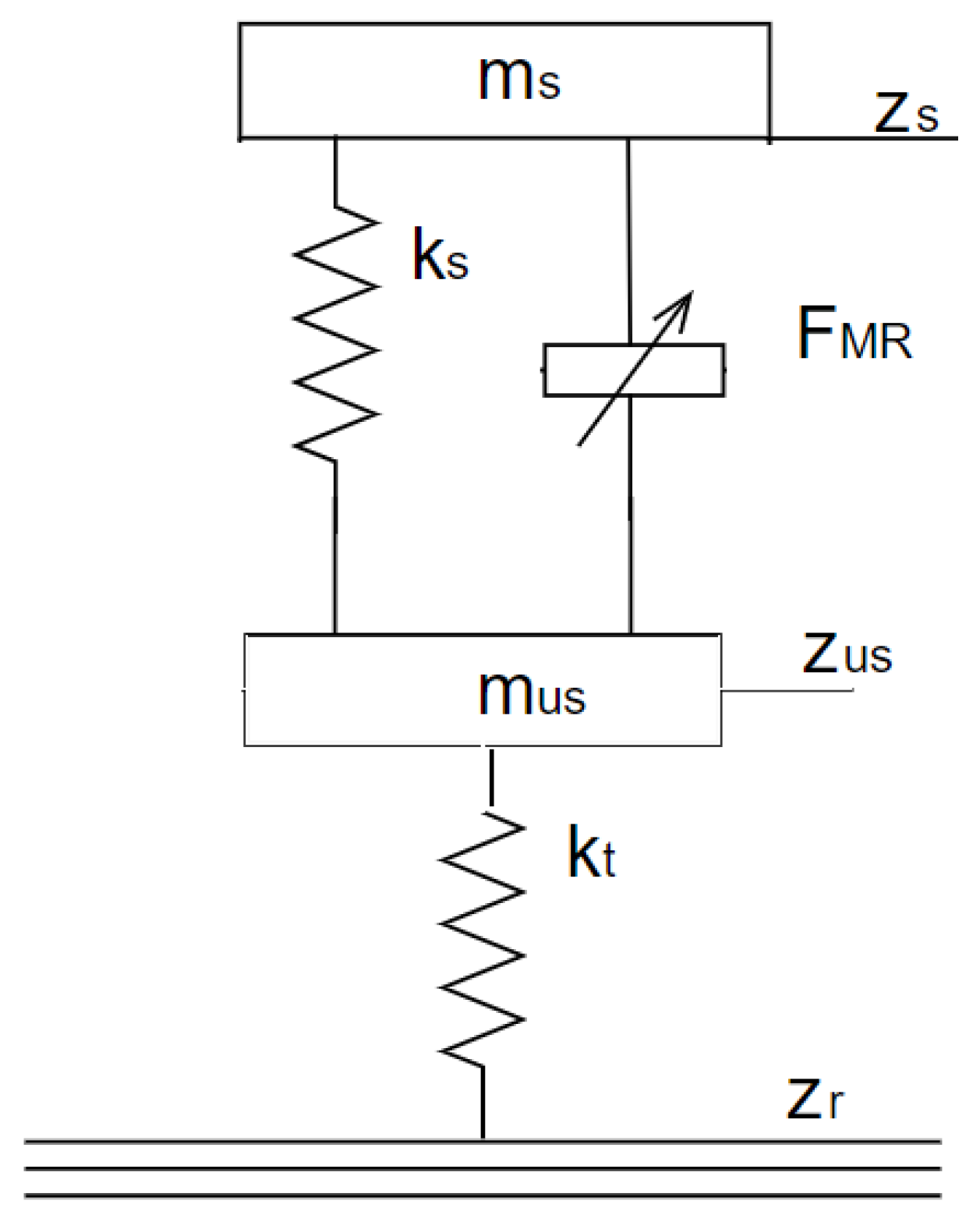
4. Application to a Semi-Active Automotive Suspension

A semi-active suspension composed by a magnetorheological (MR) damper is represented in Figure 1. The system is represented by the following mathematical model [34]:

$$\begin{array}{c}{m}_s{\ddot{z}}_s\left(t\right)=-k_s(z_s\left(t\right)-z_{us}\left(t\right))-F_{MR}\left(t\right)\end{array}$$

(32)

$$\begin{array}{cc}\hfill m_{us}{\ddot{z}}_{us}\left(t\right)& =k_s(z_s\left(t\right)-z_{us}\left(t\right))-k_t(z_{us}\left(t\right)-z_r\left(t\right))+F_{MR}\left(t\right)\hfill \end{array}$$

(33)

The semi-active damping force ($F_{MR}\left(t\right)$), with the inclusion of a manipulation signal (electric current) is represented as follows:

$$F_{MR}\left(t\right)=I{f}_c\rho \left(t\right)+b_1{\dot{z}}_{def}\left(t\right)+b_2{z}_{def}\left(t\right)+\eta \left(t\right)$$

(34)

where $\rho$ is the nonlinear part representing the hysteresis of the force provided by the magnetorheological damper [35]. Such non-linearity is described by:

$$\rho \left(t\right)=tanh(a_1{\dot{z}}_{def}\left(t\right)+a_2{z}_{def}\left(t\right))$$

(35)

The nomenclature of the parameters and variables of the model is described in

Table 1. List of parameters and variables of the mathematical model.

Parameter	Description	Value	Units
$a_1$, $a_2$	Pre-effort zone of $F_{MR}$	$37.8$, $22.15$	(Ns)/m
$b_1$, $b_2$	Post-effort zone of $F_{MR}$	$2830.86$, $-7897.21$	(Ns)/m
$f_c$	Damping force	$600.95$	N/A
I	Electric current	2	A
$k_s$	Spring stiffness coefficient	86,378	N/m
$k_t$	Tire stiffness coefficient	260,000	N/m
$m_s,m_{us}$	Suspended mass and Unsprung (tire) mass	470, 110	kg
Variable	Description	Role	Units
$z_{def}$	Vertical damper position	output $y_3$	m
$\dot{z_{def}}$	Vertical damper speed	${\dot{y}}_3$	m/s
$z_r$	Road profile	input	m
$z_s, z_{us}$	Vertical displacement of $m_s$, $m_{us}$	outputs $y_1$ and $y_2$	m
${\dot{z}}_s, {\dot{z}}_{us}$	Vertical speed of $m_s$, $m_{us}$	state $x_2$ and $x_4$	m/s
${\ddot{z}}_s, {\ddot{z}}_{us}$	Vertical acceleration of $m_s$, $m_{us}$	${\dot{x}}_2$ and ${\dot{x}}_4$	m2/s
$\rho$	Shock absorber hysteresis	nonlinear function
$F_{MR}$	Force MR	damping force	N

.

The measured outputs are $y_1\left(t\right)=z_s\left(t\right)$, $y_2\left(t\right)=z_{us}\left(t\right)$ and $y_3\left(t\right)=z_s\left(t\right)-z_{us}\left(t\right)=z_{def}\left(t\right)$. In addition, consider the following change of variables: $x_1\left(t\right)=z_s\left(t\right)$, $x_2\left(t\right)={\dot{z}}_s\left(t\right)={\dot{x}}_1\left(t\right)$, ${\dot{x}}_2\left(t\right)={\ddot{z}}_s\left(t\right)$, $x_3\left(t\right)=z_{us}\left(t\right)$, $x_4\left(t\right)={\dot{z}}_{us}\left(t\right)={\dot{x}}_3\left(t\right)$ and ${\dot{x}}_4\left(t\right)={\ddot{z}}_{us}\left(t\right)$.

The model given by Equations (32) and (33) can be rewritten as follows:

$$\begin{array}{cc}\hfill {\dot{x}}_1\left(t\right)=& x_2\left(t\right)\hfill \\ \hfill {\dot{x}}_2\left(t\right)=& - \frac{b_2+k_s}{m_s}{x}_1\left(t\right)-\frac{b_1}{m_s}{x}_2\left(t\right)+\frac{b_2+k_s}{m_s}{x}_3\left(t\right)\hfill \\ & + \frac{b_1}{m_s}{x}_4\left(t\right)-\frac{f_c\rho }{m_s}I\left(t\right)-\frac{1}{m_s}\eta \left(t\right)\hfill \\ \hfill {\dot{x}}_3\left(t\right)=& x_4\left(t\right)\hfill \\ \hfill {\dot{x}}_4\left(t\right)=& \frac{b_2+k_s}{m_{us}}{x}_1\left(t\right)+\frac{b_1}{m_{us}}{x}_2\left(t\right)-\frac{b_2+k_s+k_t}{m_{us}}{x}_3\left(t\right)\hfill \\ & - \frac{b_1}{m_{us}}{x}_4\left(t\right)+\frac{f_c\rho }{m_{us}}I\left(t\right)+\frac{1}{m_{us}}\eta \left(t\right)\hfill \\ & + \frac{k_t}{m_{us}}{z}_r\left(t\right)\hfill \end{array}$$

(36)

The state, the output, and the input vectors are $x\left(t\right)={\left[x_1\left(t\right)x_2\left(t\right)x_3\left(t\right)x_4\left(t\right)\right]}^T$, $y\left(t\right)={\left[y_1\left(t\right)y_2\left(t\right)y_3\left(t\right)\right]}^T$, $u\left(t\right)={\left[\eta \left(t\right)I\left(t\right)z_r\left(t\right)\right]}^T$, where $x_1\left(t\right)$ and $x_2\left(t\right)$ are the vertical chassis position and the vertical chassis speed, $x_3\left(t\right)$ and $x_4\left(t\right)$ are the vertical tire position and the vertical tire speed, $y_1\left(t\right)$ is the vertical chassis position, $y_2\left(t\right)$ is the vertical tire position and $y_3\left(t\right)$ is the vertical damper position, $z_r\left(t\right)$ is the road profile, and $\eta \left(t\right)$ represents a disturbance in the damper. This disturbance occurs when driving on a road with potholes and bumps, as well as due to excess luggage or passengers getting into the car. A damaged shock absorber causes an imbalance in the chassis and increases the undesirable pitching and rolling motion of the car.

Equation (36) can be represented in the form of system (1):

$$\begin{array}{c}\underset{\dot{x}}{\underbrace{\left[\begin{array}{c}{\dot{x}}_1\\ {\dot{x}}_2\\ {\dot{x}}_3\\ {\dot{x}}_4\end{array}\right]}}=\underset{A}{\underbrace{\left[\begin{array}{cccc}0& 1& 0& 0\\ -{\displaystyle \frac{b_2+k_s}{m_s}}& -{\displaystyle \frac{b_1}{m_s}}& {\displaystyle \frac{b_2+k_s}{m_s}}& {\displaystyle \frac{b_1}{m_s}}\\ 0& 0& 0& 1\\ {\displaystyle \frac{b_2+k_s}{m_{us}}}& {\displaystyle \frac{b_1}{m_{us}}}& -{\displaystyle \frac{b_2+k_s}{m_{us}}}& -{\displaystyle \frac{b_1}{m_{us}}}\end{array}\right]}}\underset{x}{\underbrace{\left[\begin{array}{c}{x}_1\\ x_2\\ x_3\\ x_4\end{array}\right]}}\\ + \underset{\Psi (y,u)}{\underbrace{\left[\begin{array}{c}0\\ -{\displaystyle \frac{f_c\rho }{m_s}}I\\ 0\\ {\displaystyle \frac{f_c\rho }{m_{us}}}I\end{array}\right]}}+\underset{\Phi (x,u,\theta )}{\underbrace{\underset{B}{\underbrace{\left[\begin{array}{c}0\\ 0\\ 0\\ 1\end{array}\right]}}\underset{{\Phi }_2(x_3,u)}{\underbrace{\left[\begin{array}{c}{\displaystyle \frac{z_r-x_3}{m_{us}}}\end{array}\right]}}\underset{k_t}{\underbrace{\theta }}}}+\underset{N}{\underbrace{\left[\begin{array}{c}0\\ -{\displaystyle \frac{1}{m_s}}\\ 0\\ {\displaystyle \frac{1}{m_{us}}}\end{array}\right]}}\eta \end{array}$$

(37)

$$\begin{array}{c}\hfill \underset{y}{\underbrace{\left[\begin{array}{c}{y}_1\\ y_2\\ y_3\end{array}\right]}}=\underset{C}{\underbrace{\left[\begin{array}{cccc}1& 0& 0& 0\\ 0& 0& 1& 0\\ 1& 0& -1& 0\end{array}\right]}}\underset{x}{\underbrace{\left[\begin{array}{c}{x}_1\\ x_2\\ x_3\\ x_4\end{array}\right]}}\end{array}$$

(38)

It can be seen in Equation (38) that function $\Phi (x,u,\theta )$ is:

$$\Phi (x,u,\theta )=\left[\begin{array}{c}{\varphi }_1(x,u,\theta )\\ {\varphi }_2(x,u,\theta )\\ {\varphi }_3(x,u,\theta )\\ {\varphi }_4(x,u,\theta )\end{array}\right]=\left[\begin{array}{c}0\\ 0\\ 0\\ {\displaystyle \frac{z_r-x_3}{m_{us}}\theta }\end{array}\right]$$

In order to verify Assumption 2, the Lipschitz constant $\gamma$ of function $\Phi (x,u,\theta )$ is computed as follows (see Lemma 3.1 in [36]):

$$\gamma ={∥\frac{\partial \Phi (x,u,\theta )}{\partial x}∥}_1={∥\begin{array}{cccc}0& 0& 0& 0\\ 0& 0& 0& 0\\ 0& 0& 0& 0\\ 0& 0& {\displaystyle -\frac{1}{m_{us}}}& 0\end{array}∥}_1=\frac{1}{m_{us}}$$

The nonlinear function $\Phi (x,u,\theta )$ satisfies the Lipschitz condition with respect to the state variables [7]. Assumption 3 is also verified. The Lipschitz constant of function ${\Phi }_2(x_3,u)\in \mathbb{R}$ is the same as the Lipschitz constant of function $\Phi (x,u,\theta )$, i.e.,:

$${∥\frac{\partial {\Phi }_2(x_3,u)}{\partial x_3}∥}_1=\frac{1}{m_{us}}$$

Therefore, the observer (4) is used to simultaneously estimate the state variables and the unknown parameter $\theta$.

By considering that the parameter to be estimated is the spring stiffness coefficient $k_t$, then the observer (4) for system (37) is

$$\begin{array}{c}\underset{\dot{\widehat{x}}}{\underbrace{\left[\begin{array}{c}{\dot{\widehat{x}}}_1\\ {\dot{\widehat{x}}}_2\\ {\dot{\widehat{x}}}_3\\ {\dot{\widehat{x}}}_4\end{array}\right]}}=\underset{A}{\underbrace{\left[\begin{array}{cccc}0& 1& 0& 0\\ -{\displaystyle \frac{b_2+k_s}{m_s}}& -{\displaystyle \frac{b_1}{m_s}}& {\displaystyle \frac{b_2+k_s}{m_s}}& {\displaystyle \frac{b_1}{m_s}}\\ 0& 0& 0& 1\\ {\displaystyle \frac{b_2+k_s}{m_{us}}}& {\displaystyle \frac{b_1}{m_{us}}}& -{\displaystyle \frac{b_2+k_s}{m_{us}}}& -{\displaystyle \frac{b_1}{m_{us}}}\end{array}\right]}}\underset{\widehat{x}}{\underbrace{\left[\begin{array}{c}{\widehat{x}}_1\\ {\widehat{x}}_2\\ {\widehat{x}}_3\\ {\widehat{x}}_4\end{array}\right]}}\\ + \underset{\Psi (y,u)}{\underbrace{\left[\begin{array}{c}0\\ {\displaystyle -\frac{f_c\rho }{m_s}I}\\ 0\\ {\displaystyle \frac{f_c\rho }{m_{us}}I}\end{array}\right]}}+\underset{\Phi (\widehat{x},u,\theta )}{\underbrace{\underset{B}{\underbrace{\left[\begin{array}{c}0\\ 0\\ 0\\ 1\end{array}\right]}}\underset{{\Phi }_2({\widehat{x}}_3,u)}{\underbrace{\left[\begin{array}{c}{\displaystyle \frac{z_r-{\widehat{x}}_3}{m_{us}}}\end{array}\right]}}\underset{k_t}{\underbrace{\widehat{\theta }}}}}+L(y-C\widehat{x})\end{array}$$

$$\begin{array}{c}\hfill \dot{\widehat{\theta }}=\Gamma {\left[\begin{array}{c}{\displaystyle \frac{z_r-{\widehat{x}}_3}{m_{us}}}\end{array}\right]}^{T}H(y-C\widehat{x})\end{array}$$

The matrices L and H are the gains of the observer, and they must be selected to guarantee the estimation convergence of the estimated states and parameters. The gain $\Gamma >0$ is a positive scalar. In this case, $\Gamma =125$ is chosen, because this value allows an adequate convergence time for the observer.

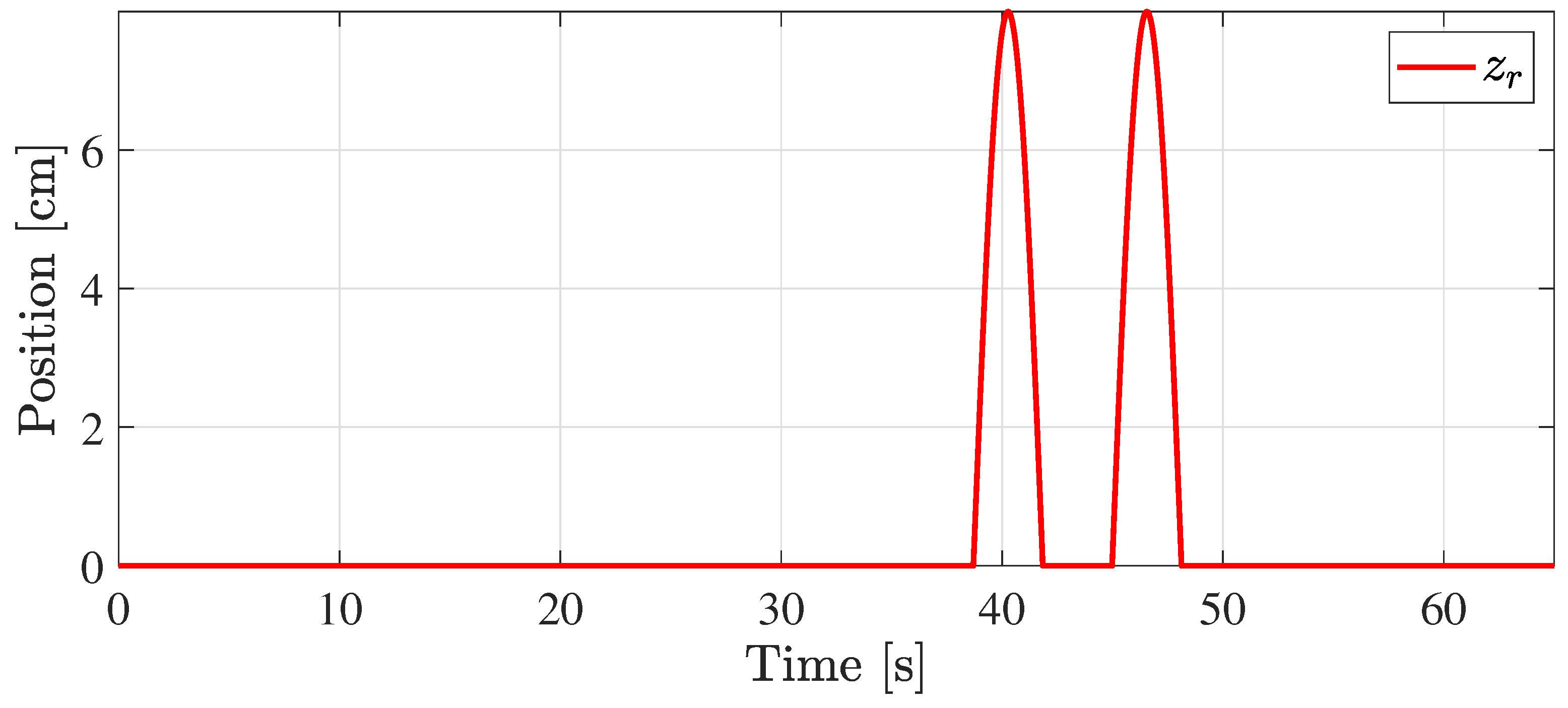
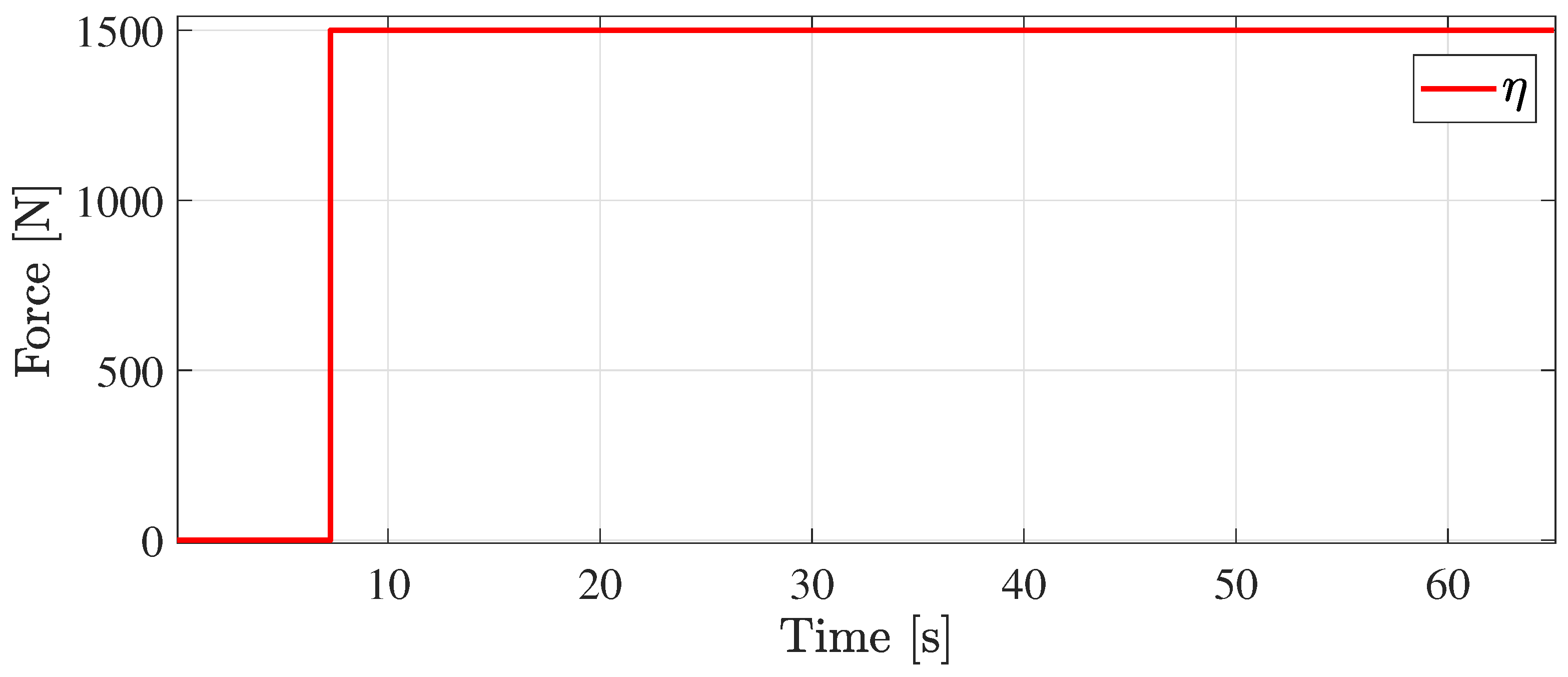
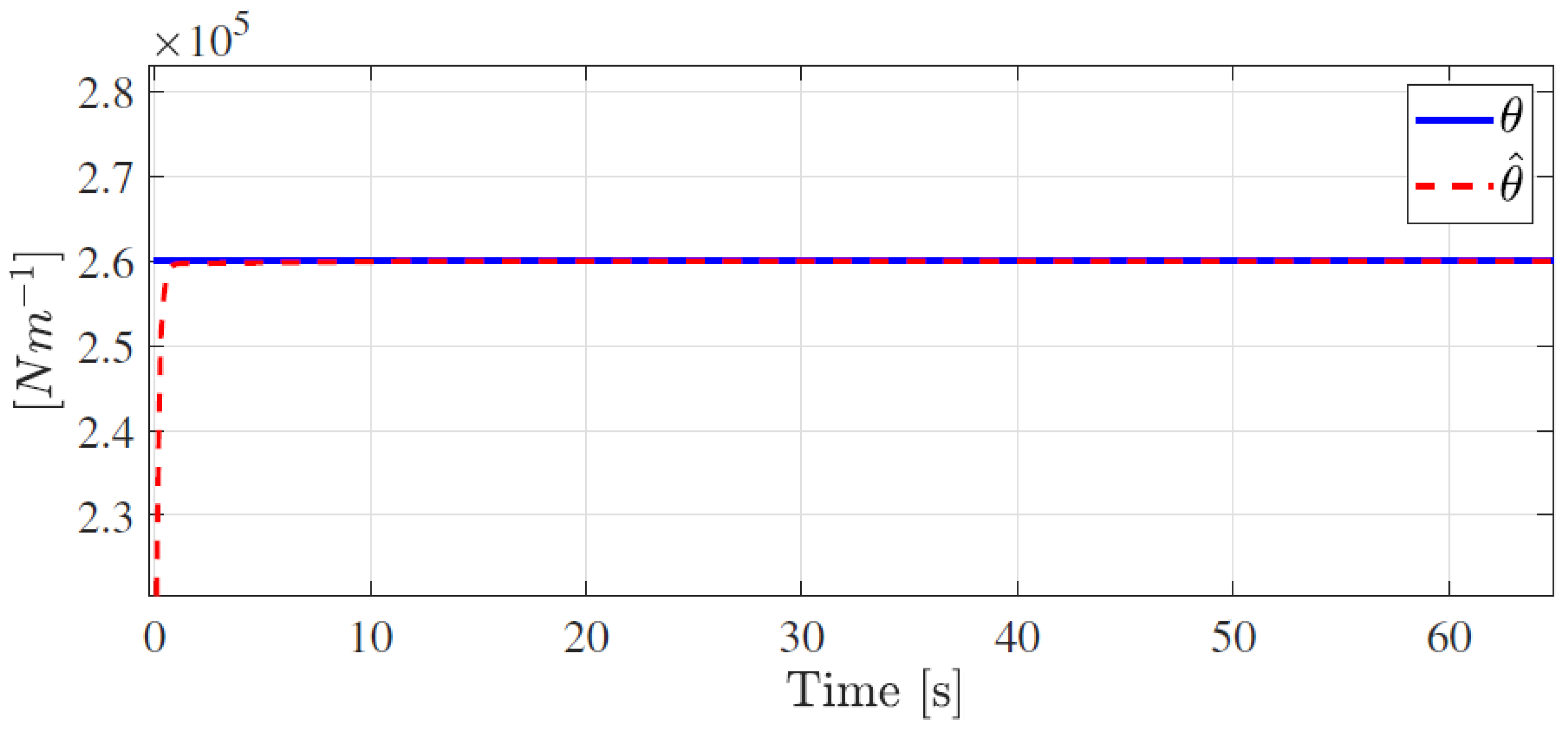
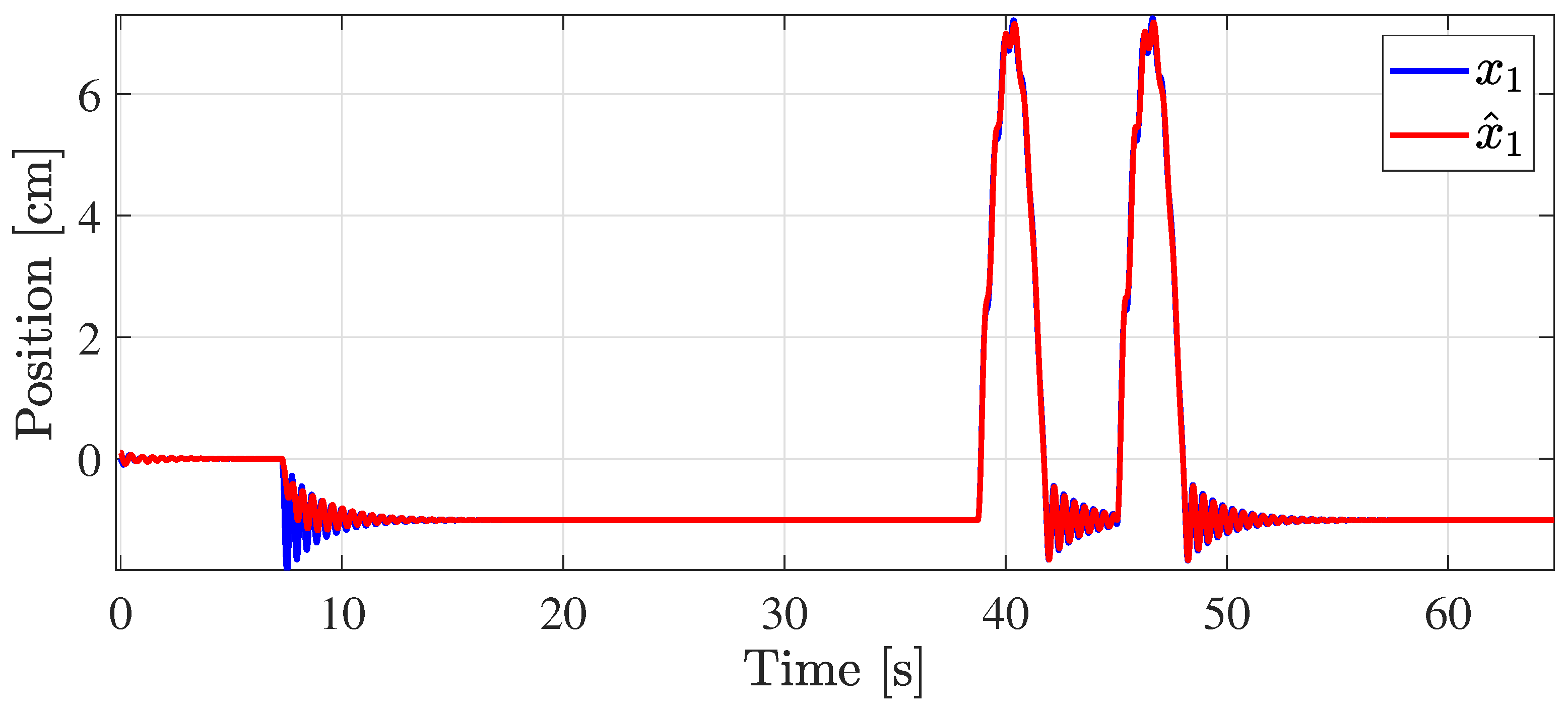
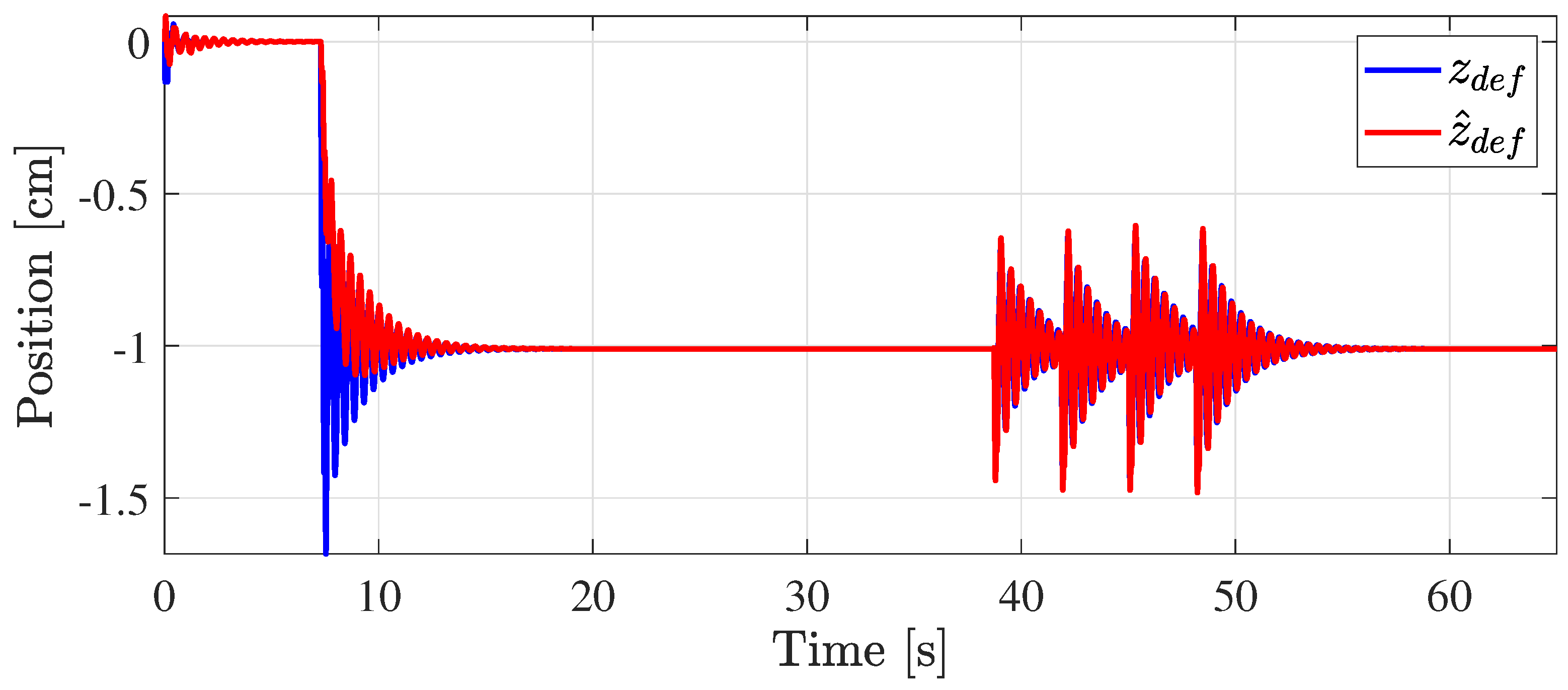
5. Simulation Results

To evaluate the performance of the proposed observer, the behavior of the suspension was analyzed when a disturbance occurs in the damping force $\eta \left(t\right)$, affecting the position of the piston, causing poor vehicle comfort, and risk of rollover due to disturbances on the road $z_r\left(t\right)$. The parameters presented in Table 1 were considered to estimate the unknown parameter $k_t$, which represents the stiffness of the tire. The simulation was implemented using MATLAB, with a simulation time of 65 s. This time frame was chosen to ensure the system stabilized adequately before any subsequent disturbances or inputs could affect it again. The first-order Euler method was used to integrate the differential equations, with an integration step of 1ms. The initial conditions of the system and the observer were $x\left(0\right)={\left[0000\right]}^T$ and $\widehat{x}\left(0\right)={\left[0.10.10.10.1\right]}^T$. The electric current was $I\left(t\right)=2$ A.

A road profile was assumed starting as a straight path, and then it passed through two consecutive speed bumps and finally it continued with its path $z_r\left(t\right)$ as shown in Figure 2. This road profile was considered as an input $z_r\left(t\right)$. It can be appreciated that each bump on the road exerted a vertical force on the vehicle during 3 s, affecting the vertical positions $x_1$, $x_3$ and $z_{def}$.

The system had a disturbance in the actuator $\eta \left(t\right)$. The disturbance profile, shown in Figure 3, corresponds to around $15\%$ of the shock absorber’s operating range, thereby affecting the comfort and safety of passengers. This disturbance influences the position of the shock absorber piston gradually, diminishing its ability to dampen the vehicle oscillations resulting from road irregularities.

The observer gains were obtained by solving the LMI presented in Equation (17) using the MATLAB toolbox YALMIP:

$$\begin{array}{cc}\hfill L=& \left[\begin{array}{ccc}-0.9627& -0.9677& 0.0050\\ 1.3959& -1.0688& 2.4647\\ -0.6003& -0.5931& -0.0072\\ -1.0688& 1.3799& -2.4487\end{array}\right]\hfill \end{array}$$

(39)

$$\begin{array}{c}H=\left[\begin{array}{ccc}-0.3696& -0.3708& 0.0012\end{array}\right]\end{array}$$

(40)

As shown in Figure 4, the unknown parameter $\theta =k_t$ was adequately estimated with appropriate time convergence.

Once the parameter $k_t$ had been estimated, the observer was able to estimate the position of the chassis $x_1$ and its estimated value ${\widehat{x}}_1$ (Figure 5). The effect of the disturbance $\eta$ was observed at $t=8$ s. This harmed the comfort and safety of passengers. The observer attenuated the effect of the disturbance by minimizing the oscillation of ${\widehat{x}}_1$. It can be seen that the disturbance caused an alteration in the behavior of the shock absorber when the vehicle went over speed bumps on the road.

The position of the tire $x_3$ and its estimated value ${\widehat{x}}_3$ are shown in Figure 6.

It can be seen that the effect of the disturbance $\eta$ on the damper caused oscillations, which forced the tire to follow the path over speed bumps on the road. Once again, the observer attenuated the oscillation of ${\widehat{x}}_3$, obtaining an adequate estimation of the output despite the presence of the disturbance.

Knowing the positions of the chassis and the tire, the vertical position of the shock absorber could be calculated (as seen in Figure 7). One can observe the effect of the disturbance on the actuator when the tire passed over the road profile, allowing us to minimize the disturbance to our observer.

The behavior of the suspension was affected by the disturbance $\eta$. The greater the force that disturbed the shock absorber, the greater its deformation. The observer estimated the tire’s stiffness coefficient $k_t$ to monitor the deterioration of the tire and managed to attenuate the disturbance.

6. Conclusions

An ${\mathcal{H}}_{\infty }$ adaptive observer was presented for processes that can be modeled as nonlinear Lipschitz systems. The proposed conditions under a passivity constraint were employed to deal with nonlinear systems with certain unknown parameters. The proposed observer was able to simultaneously estimate unknown states and parameters, even in the presence of disturbances. The main advantage of this observer is that it can be applied to a wider class of systems with unknown parameters. Moreover, by incorporating the ${\mathcal{H}}_{\infty }$ criteria into the design, the observer demonstrated enhanced resilience against undesired disturbances, while ensuring robust performance. Unlike high-gain observers, the observer design process does not necessitate a coordinate transformation, thereby streamlining implementation and reducing complexity. A semi-active car suspension was used to test the performance of the proposed observer. Thanks to the ${\mathcal{H}}_{\infty }$ approach, the effect of disturbances or unknown inputs could be attenuated, allowing for better monitoring of the systems. The simplicity of computing the observer gains was demonstrated, eliminating the need to solve the additional differential equations usually associated with Kalman observers. It is well known that Kalman observers (or filters as presented in [29,30]) require additional differential equations to recursively compute the observer gain, incorporating the predicted covariance matrix to estimate the accuracy of state estimates (e.g., [37]). In contrast, the proposed observer employs fixed-value observer gains, which are computed offline once, by solving the LMIs provided in Theorem 1. The simulation results demonstrated the effectiveness of the proposed approach in dealing with a practical system. As future work, we expect to apply the ${\mathcal{H}}_{\infty }$ approach at the output to supervise the operation of dynamic systems in the presence of sensor disturbances.

Future work will focus on developing adaptive observers for non-Lipschitz nonlinear systems, such as those involving dry friction. This approach aims to broaden the scope and address more realistic scenarios.

References

1. Thau, F. Observing the state of non-linear dynamic systems. Int. J. Control 1973, 17, 471–479. [Google Scholar] [CrossRef]
2. Zemouche, A.; Rajamani, R.; Trinh, H.; Zasadzinski, M. A new LMI based H observer design method for Lipschitz nonlinear systems. In Proceedings of the 2016 European Control Conference (ECC), Aalborg, Denmark, 29 June–1 July 2016; pp. 2011–2016. [Google Scholar]
3. Zemouche, A.; Rajamani, R.; Kheloufi, H.; Bedouhene, F. Robust observer-based stabilization of Lipschitz nonlinear uncertain systems via LMIs-discussions and new design procedure. Int. J. Robust Nonlinear Control 2017, 27, 1915–1939. [Google Scholar] [CrossRef]
4. Shaheen, B.; Nazir, M.S.; Rehan, M.; Ahmad, S. Robust generalized observer design for uncertain one-sided Lipschitz systems. Appl. Math. Comput. 2020, 365, 124588. [Google Scholar] [CrossRef]
5. Wang, X.; Park, J.H. State-Based Dynamic Event-Triggered Observer for One-Sided Lipschitz Nonlinear Systems with Disturbances. IEEE Trans. Circuits Syst. II Express Briefs 2022, 69, 2326–2330. [Google Scholar] [CrossRef]
6. Mu, Y.; Zhang, H.; Yan, Y.; Wu, Z. A design framework of nonlinear H PD observer for one-sided Lipschitz singular systems with disturbances. IEEE Trans. Circuits Syst. II Express Briefs 2022, 69, 3304–3308. [Google Scholar] [CrossRef]
7. Besançon, G. Remarks on nonlinear adaptive observer design. Syst. Control Lett. 2000, 41, 271–280. [Google Scholar] [CrossRef]
8. Zhang, J.; Swain, A.K.; Nguang, S.K. Robust H adaptive descriptor observer design for fault estimation of uncertain nonlinear systems. J. Frankl. Inst. 2014, 351, 5162–5181. [Google Scholar] [CrossRef]
9. Wang, H.; Wang, Q.; Zhang, H.; Han, J. H-Infinity Observer for Vehicle Steering System with Uncertain Parameters and Actuator Fault. Actuators 2022, 11, 43. [Google Scholar] [CrossRef]
10. Mu, Y.; Zhang, H.; Ren, H.; Cai, Y. Fuzzy adaptive observer-based fault and disturbance reconstructions for TS fuzzy systems. IEEE Trans. Circuits Syst. II Express Briefs 2021, 68, 2453–2457. [Google Scholar]
11. Xiong, X.; Pal, A.K.; Liu, Z.; Kamal, S.; Huang, R.; Lou, Y. Discrete-time adaptive super-twisting observer with predefined arbitrary convergence time. IEEE Trans. Circuits Syst. II Express Briefs 2020, 68, 2057–2061. [Google Scholar] [CrossRef]
12. Qin, Q.; Gao, G.; Zhong, J. Finite-Time Adaptive Extended State Observer-Based Dynamic Sliding Mode Control for Hybrid Robots. IEEE Trans. Circuits Syst. II Express Briefs 2022, 69, 3784–3788. [Google Scholar] [CrossRef]
13. Li, W.; Yao, X.; Krstic, M. Adaptive-gain observer-based stabilization of stochastic strict-feedback systems with sensor uncertainty. Automatica 2020, 120, 109112. [Google Scholar] [CrossRef]
14. Yan, S.; Sun, W.; Yu, X.; Gao, H. Adaptive Sensor Fault Accommodation for Vehicle Active Suspensions via Partial Measurement Information. IEEE Trans. Cybern. 2021, 52, 12290–12301. [Google Scholar] [CrossRef] [PubMed]
15. Bzioui, S.; Channa, R. An Adaptive Observer Design for Nonlinear Systems Affected by Unknown Disturbance with Simultaneous Actuator and Sensor Faults. Application to a CSTR. Biointerface Res. Appl. Chem. 2021, 12, 4847–4856. [Google Scholar]
16. Bonargent, T.; Menard, T.; Gehan, O.; Pigeon, E. Adaptive observer design for a class of Lipschitz nonlinear systems with multirate outputs and uncertainties: Application to attitude estimation with gyro bias. Int. J. Robust Nonlinear Control 2021, 31, 3137–3162. [Google Scholar] [CrossRef]
17. Zheng, Y.; Liu, Y.; Song, R.; Ma, X.; Li, Y. Adaptive neural control for mobile manipulator systems based on adaptive state observer. Neurocomputing 2022, 489, 504–520. [Google Scholar] [CrossRef]
18. Sleiman, M.; Bouyekhf, R.; Al Chami, Z.; El Moudni, A. Uncertainty observer and stabilization for transportation network with constraints. J. Appl. Math. Comput. 2022, 68, 1107–1133. [Google Scholar] [CrossRef]
19. Perrier, M.; De Azevedo, S.F.; Ferreira, E.; Dochain, D. Tuning of observer-based estimators: Theory and application to the on-line estimation of kinetic parameters. Control Eng. Pract. 2000, 8, 377–388. [Google Scholar] [CrossRef]
20. Astorga, C.M.; Othman, N.; Othman, S.; Hammouri, H.; McKenna, T.F. Nonlinear continuous–discrete observers: Application to emulsion polymerization reactors. Control Eng. Pract. 2002, 10, 3–13. [Google Scholar] [CrossRef]
21. Arcak, M.; Gorgun, H.; Pedersen, L.M.; Varigonda, S. A nonlinear observer design for fuel cell hydrogen estimation. IEEE Trans. Control Syst. Technol. 2004, 12, 101–110. [Google Scholar] [CrossRef]
22. Astorga-Zaragoza, C.M.; Zavala-Río, A.; Alvarado, V.; Méndez, R.M.; Reyes-Reyes, J. Performance monitoring of heat exchangers via adaptive observers. Measurement 2007, 40, 392–405. [Google Scholar] [CrossRef]
23. Ramos-Hernández, E.; Astorga-Zaragoza, C.; Reyes, J.R.; Ramırez-Rasgado, F.; Osorio-Gordillo, G.; Ruiz-Acosta, S. Estimation of Process Variables in a Steam Distillation Plant. Congreso Nacional de Control Automático. 2023. Available online: https://revistadigital.amca.mx/wp-content/uploads/2023/12/0103.pdf (accessed on 29 May 2024).
24. Farza, M.; M’saad, M.; Menard, T.; Ltaief, A.; Maatoug, T. Adaptive observer design for a class of nonlinear systems. Application to speed sensorless induction motor. Automatica 2018, 90, 239–247. [Google Scholar] [CrossRef]
25. Dong, Z.; Liu, M.; Guo, Z.; Huang, X.; Zhang, Y.; Zhang, Z. Adaptive state-observer for monitoring flexible nuclear reactors. Energy 2019, 171, 893–909. [Google Scholar] [CrossRef]
26. Zhong, J.; Feng, Y.; Chen, X.; Zeng, C. Observer-based piecewise control of reaction–diffusion systems with the non-collocated output feedback. J. Appl. Math. Comput. 2023, 69, 4187–4211. [Google Scholar] [CrossRef]
27. de Jesús Rubio, J.; Lughofer, E.; Pieper, J.; Cruz, P.; Martinez, D.I.; Ochoa, G.; Islas, M.A.; Garcia, E. Adapting H-infinity controller for the desired reference tracking of the sphere position in the Maglev process. Inf. Sci. 2021, 569, 669–686. [Google Scholar] [CrossRef]
28. Asad, M.; Rehan, M.; Ahn, C.K.; Tufail, M.; Basit, A. Distributed H State and Parameter Estimation over Wireless Sensor Networks under Energy Constraints. IEEE Trans. Netw. Sci. Eng. 2024, 11, 2976–2988. [Google Scholar] [CrossRef]
29. Chen, C.; Sun, F.; Xiong, R.; He, H. A Novel Dual H Infinity Filters Based Battery Parameter and State Estimation Approach for Electric Vehicles Application. Energy Procedia 2016, 103, 375–380. [Google Scholar] [CrossRef]
30. Gong, X.; Suh, J.; Lin, C. A novel method for identifying inertial parameters of electric vehicles based on the dual H infinity filter. Veh. Syst. Dyn. 2019, 58, 28–48. [Google Scholar] [CrossRef]
31. Xu, S. Robust H filtering for a class of discrete-time uncertain nonlinear systems with state delay. IEEE Trans. Circuits Syst. I Fundam. Theory Appl. 2002, 49, 1853–1859. [Google Scholar]
32. Ekramian, M.; Hosseinnia, S.; Sheikholeslam, F. Observer design for non-linear systems based on a generalised Lipschitz condition. IET Control Theory Appl. 2011, 5, 1813–1818. [Google Scholar] [CrossRef]
33. Ekramian, M.; Sheikholeslam, F.; Hosseinnia, S.; Yazdanpanah, M.J. Adaptive state observer for Lipschitz nonlinear systems. Syst. Control Lett. 2013, 62, 319–323. [Google Scholar] [CrossRef]
34. Guo, S.; Yang, S.; Pan, C. Dynamic modeling of magnetorheological damper behaviors. J. Intell. Mater. Syst. Struct. 2006, 17, 3–14. [Google Scholar] [CrossRef]
35. Tudon-Martinez, J.C.; Morales-Menéndez, R.; Ramirez-Mendoza, R.; Sename, O.; Dugard, L. Fault tolerant control in a semi-active suspension. IFAC Proc. Vol. 2012, 45, 1173–1178. [Google Scholar] [CrossRef]
36. Khalil, H.K.; Grizzle, J.W. Nonlinear Systems; Prentice Hall: Upper Saddle River, NJ, USA, 2002; Volume 3, Available online: https://nasim.hormozgan.ac.ir/ostad/UploadedFiles/863740/863740-8707186354456456.pdf (accessed on 29 May 2024).
37. Zhao, J.; Mili, L. A decentralized H-infinity unscented Kalman filter for dynamic state estimation against uncertainties. IEEE Trans. Smart Grid 2018, 10, 4870–4880. [Google Scholar] [CrossRef]
Figure 1. Semi-active suspension diagram.
Mca 29 00051 g001
Figure 2. Road profile z r : a straight path and two speed bumps.
Mca 29 00051 g002
Figure 3. Disturbance η affecting the semi-active damping force F M R ( t ) (see Equation (34)).
Mca 29 00051 g003
Figure 4. Simulated wheel stiffness coefficient θ (solid line) and its estimation value θ ^ (dotted line).
Mca 29 00051 g004
Figure 5. Chassis vertical position x 1 (blue line) and its estimated value x ^ 1 (red line).
Mca 29 00051 g005
Figure 6. Tire vertical position x 3 (blue line) and its estimated value x ^ 3 (red line).
Mca 29 00051 g006
Figure 7. Vertical damper position z d e f (blue line) and its estimated value z ^ d e f (red line).
Mca 29 00051 g007