Abstract
This paper presents a mathematical model of the cardiovascular system (CVS) designed to simulate both normal and pathological conditions within the systemic circulation. The model introduces a novel representation of the CVS through a change of coordinates, transforming it into the “quadratic normal form”. This model facilitates the implementation of a sliding mode observer (SMO), allowing for the estimation of system states and the detection of anomalies, even though the system is linearly unobservable. The primary focus is on identifying valvular heart diseases, which are significant risk factors for cardiovascular diseases. The model’s validity is confirmed through simulations that replicate hemodynamic parameters, aligning with existing literature and experimental data.
1. Introduction
The World Health Organization (WHO) has reported that cardiovascular diseases (CVDs) continue to be the world’s leading cause of mortality [1]. In clinical practice, arterial pressure () is frequently used to evaluate cardiovascular health and disease. However, it has been suggested that aortic pressure (), measured near to the heart, provides more information about health behavior and diseases compared to blood pressure measurements. Nevertheless, the widespread adoption of aortic pressure measurement faces significant challenges due to the invasive and/or inconvenient procedures required, as well as the need for skilled physicians to perform direct measurements, such as cardiac catheterization and carotid artery tonometry [2].
These challenges have spurred research on the cardiovascular system (CVS) from various perspectives, including those that diverge from traditional medical approaches. Among these perspectives are computational and mathematical models, which allow for experiments that are much simpler and less expensive to conduct than in vivo or in vitro heart experiments. Given the complexity of the cardiovascular system, interdisciplinary expertise may be helpful in developing dynamic models that can predict cardiovascular events in patients with heart failure, myocardial infarction, or valvular heart disease. Research on the CVS is ongoing, with significant efforts dedicated to modeling the CVS to better understand its behavior and to develop new, reliable diagnostic techniques [3,4,5,6]. Simplified parameter models are particularly noteworthy, as they provide streamlined representations of the primary behaviors of each CVS component [3,4,5,6,7,8,9,10,11,12]. Mathematical models have thus emerged as valuable tools, offering simpler and less expensive alternatives to in vitro heart experiments [6,13,14,15]. For systems described by dynamic models, there are methods for fault localization and detection that rely on creating fault indicators, also known as residuals. These indicators are determined by comparing actual system measurements with estimates made by an observer. Numerous results based on linear models have been published across various contexts [9,16,17,18]. While observers used to reconstruct system states have been very useful for monitoring and detecting anomalies, the implementation of observers for nonlinear models has not been extensively explored. This is particularly challenging because the design of observers is generally more sensitive when a nonlinear model is required to represent the system’s behavior. Currently, there are no straightforward, generic methods for creating observers for all types of nonlinear systems.
This work used a model of the cardiovascular system (CVS) from the study [19], designed to simulate both normal and pathological conditions within the systemic circulation. The model introduces a novel representation of the CVS by transforming it into the “quadratic normal form” through a change of coordinates. This model offers a structured approach to understanding the complexity of this system, aiding the development of clinical decision support systems for cardiovascular diseases (CVDs), and facilitates the implementation of a sliding mode observer (SMO), enabling the estimation of system states and the detection of anomalies, even though the system is linearly unobservable.
This paper is structured as follows: Section 2 provides a brief overview of CVS functionality. In Section 3, the justification for employing electrical analogies in the CVS description is discussed, along with the depiction of the CVS model and a validation of the proposed model against clinical indices and experimental data. Section 4 explores the potential of the quadratic normal form and sliding mode observer design as suitable tools for CVD modeling. Section 5 presents the CVS model designed for anomaly detection, focusing on two types of faults in the mitral and aortic valves. Simulation results are then presented to illustrate how this design can estimate system states for cardiovascular activity monitoring. Finally, Section 6 presents the conclusions.
2. Cardiovascular System Model
This section is dedicated to describing the dynamic behavior of the CV system from both a medical and control theory perspective.
2.1. Anatomy and Physiology of the Cardiac Cycle
The dynamic behavior of the cardiac cycle can be described as a distribution network of blood vessels to supply oxygenated and deoxygenated blood throughout the body, thanks to the heart behaving as a pump and its pressure–volume (PV) loops.
- Blood circulation pathway
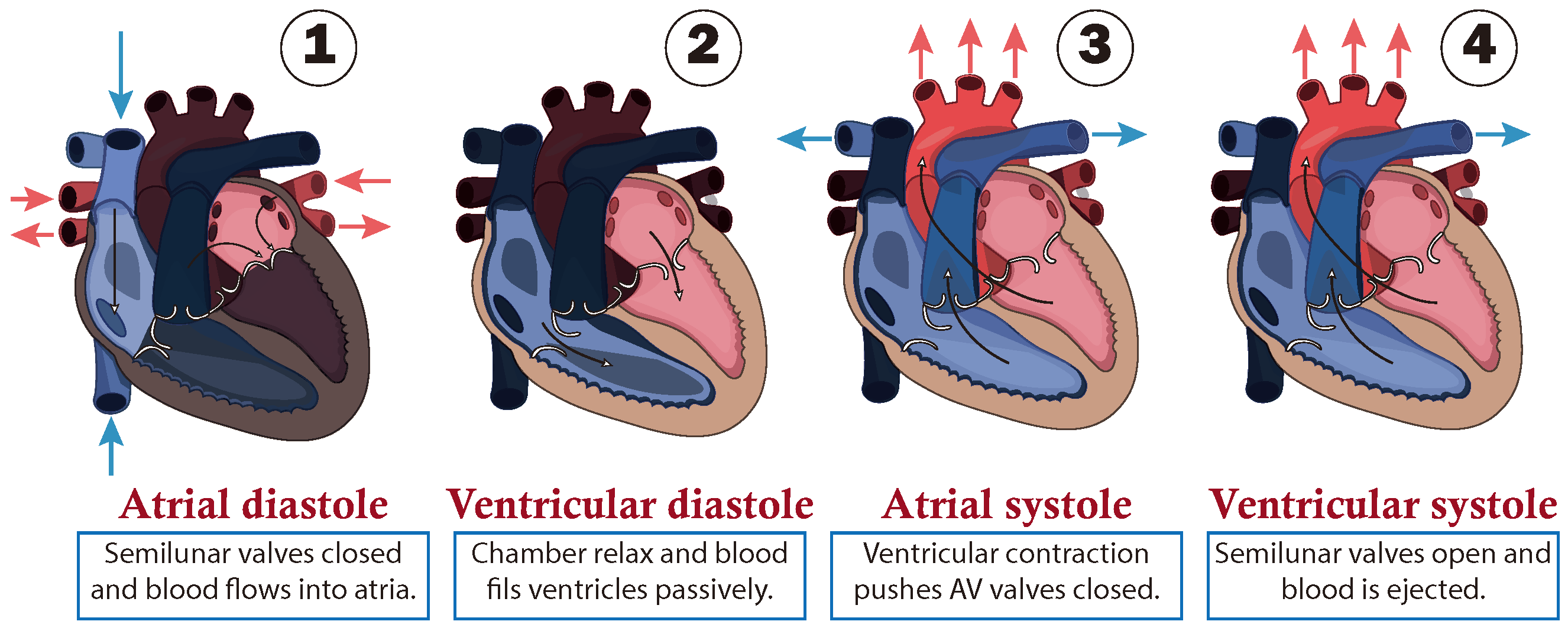
The path followed by the blood is presented as a closed circuit, starting at the heart, which is responsible for pumping blood. This is illustrated in Figure 1 through a schematic cross-section of the heart, consisting of double atria-ventricular chambers on both sides. Where, the ventricles act as the primary pumps, while the atria serve as preload chambers that regulate the distinct paths of blood circulation. Specifically, the right side of the heart regulates blood flow in to the pulmonary artery, which carries to the lungs, where blood is oxygenated in the lungs and then it returns to the left side of the heart entering through the left atrium. Subsequently, the oxygen-rich blood is pumped by the left ventricle through the aorta, regulating blood circulation to the rest of the body [20]. Additionally, it is important to note that blood flows in one direction only, due to one-way valves being situated between the chambers to prevent reflux, and at the output of the ventricles, called semilunar valves as shown in Figure 1.
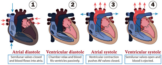
Figure 1.
Cardiac cycle of circulatory system.
- Cardiac cycle phases
From a functional point of view, the cardiac cycle is divided into two alternating phases: diastole (dilatation period) and systole (contraction period), which are simplified into four stages as shown in Figure 1:
- (1)
- The first stage is atrial diastole and the beginning of ventricular systole, during which the atria relax while the ventricles contract and the atrioventricular valves close. This increases the pressure inside the ventricles but not enough to open the semilunar valves.
- (2)
- The second stage is ventricular diastole, when the pressure inside the ventricles rapidly decreases, the atrioventricular valves open, and the chambers passively fill due to their relaxation combined with atrial systole, during which the atria contract to fill the ventricles.
- (3)
- The third stage is atrial systole, during which the pressure in the ventricles rises until it exceeds that of the arteries. This leads to the opening of the semilunar valves and the ejection of blood into the pulmonary artery, marking the beginning of systemic circulation.
- (4)
- The last stage marks the end of ventricular systole and the start of the ventricular and atrial diastole. During this phase, the pressure in the ventricles decreases rapidly, and all chambers passively fill due to their relaxation. This transition leads into a new cardiac cycle, beginning with atrial systole.
An alternative method to graphically describe and characterize the cardiac cycle is through the use of a left ventricle (PV) loop. This loop illustrates the relationship between left ventricular pressure (LVP) and left ventricular volume (LVV) across the four stages of the cardiac cycle. It enables the identification of changes in cardiac function, including the factors related to preload and afterload, as well as heart contractility (for more information see [6]).
2.2. Valve Pathologies
Valvular heart diseases are a leading cause of cardiovascular morbidity and mortality worldwide [1,21]. Among the most frequent valve pathologies are those impacting the aortic and mitral valves. These pathologies often result in both stenosis (narrowing) and regurgitation (impaired closure).
Aortic valve stenosis refers to the insufficient opening of the valve during systole, often caused by congenital abnormalities or the progressive buildup of calcium on the valve leaflets with age [6,22,23]. Conversely, a malfunction in the aortic valve closure, known as aortic valve regurgitation, results in backward leakage into the left ventricle during diastole. This condition shares similar causes with aortic valve stenosis [22].
Both aortic stenosis and regurgitation lead to the hypertrophy of the left ventricle in response to increased stress, resulting in the thickening of the left ventricular muscle and the subsequent elevation of left ventricular pressure.
3. Description of the Cardiovascular System Model
This section outlines the equivalences between electrical and hydrodynamic indices. We can simulate the CVS electrically by utilizing the equivalencies between hydrodynamic and electrical indicators. This model addresses the simulation of the system and the contractile activity of the heart once the relationships and equivalencies between an electrical circuit and the behavior defined by a segment of the CVS are established.
3.1. Equivalent Electric Model
The heart is a highly complex system that presents significant challenges for mathematical modeling. In recent years, numerous dynamical state-space models with varying levels of complexity have been developed [10]. The main methodology employed is that of lumped parameter models, which provide simplified descriptions of the predominant behavior of each component involved in the CVS [4,7,10,11,12].
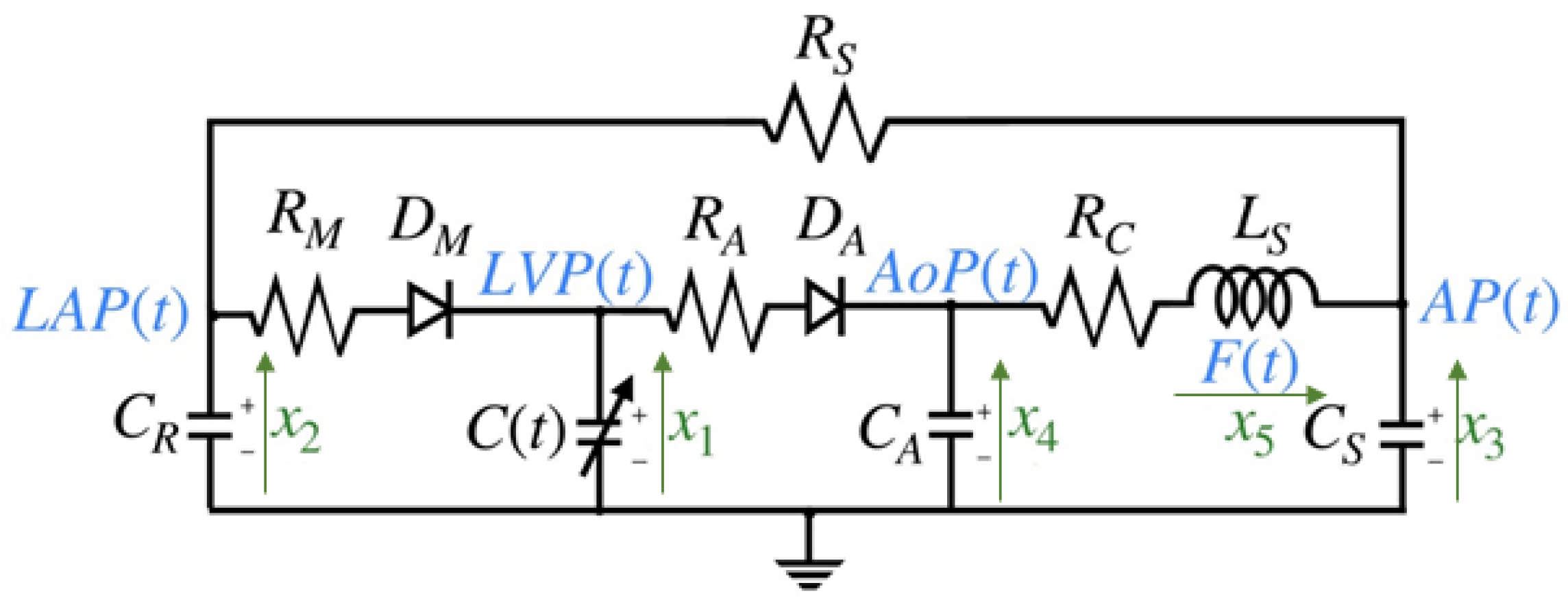
The model discussed in this work is based on an electrical representation of the CVS, as proposed in [4,7,12]. The choice of this model is motivated by the need for a comprehensive model that can be validated from a medical perspective and is capable of describing cardiovascular phenomena, such as valve pathologies, which are among the primary risk factors for cardiovascular diseases (CVDs). This model primarily targets the left chambers of the heart, assuming that voltages are analogous to pressure and currents are analogous to blood flow. The systemic resistance is the resistance to flow from the descending aorta through the capillary vessels, venous, and pulmonary circulation to reach the left atrium. Left ventricular pressure (LVP) is represented by the voltage across the time-varying contractile capacity , where its capacitance is defined as the inverse of left ventricular elastance . The term represents the elastance of the heart at time t, which is a function of the pressure. The mitral and aortic valves are represented as ideal diodes, and , in series with resistance and , respectively. The capacitor , represents the elasticity of the ascending aorta, simulating the pressure variations caused by the opening and closing of the aortic valve. Finally, the remaining components model the anatomical characteristics of the circulatory system, including the elasticity represented by , inertia (), and resistance of the descending aorta [6]. The electrical model circuit in Figure 2 has been thoroughly analyzed in [6,20].
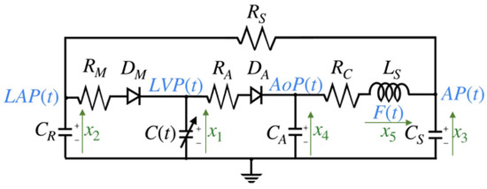
Figure 2.
Cardiovascular circuit model.
The state variables and parameter values of the cardiovascular circuit model shown in Figure 2, as referenced from [6,17,20], are detailed in Table 1 and Table 2 below:

Table 1.
State variables of the cardiovascular system and their physiological significance of the circuit model shown in Figure 2.
Table 2.
Parameter values of the CVS circuit model shown in Figure 2.
3.2. Elastance
Elastance, denoted as , relates to the state of contraction of the left ventricle. It represents the relationship between the pressure and volumes of the LV, as defined by the following expression:
where is the left ventricular pressure, is the left ventricular volume, and is a reference volume, which corresponds to the theoretical volume in the ventricle at zero pressure. The elastance function has been addressed in various studies [20]. These studies concur that the definition can be mathematically approximated using an expression where the points at which the left ventricular function reaches its maximum and minimum are identified used the expression:
where and are constants related to the end-systolic volume (ESV) and end-diastolic volume (EDV), representing the left ventricular volumes at systole and diastole, respectively. The end-systolic pressure–volume relationship (ESPVR) denotes the maximal pressure of the left ventricle.
The elastance function is implemented using a number of mathematical approximations, including , the so-called “double hill” [24]. In this paper, represents the normalized elastance at time . “Normalized” means that it has been adjusted or expanded to fit a specific range, often between 0 and 1 or and 1. The normalized elastance is scaled proportionally between and . Specifically, when , equal , and when , equal . In the context of the cardiovascular system, describes how elastance dynamically varies over time adjusted to heart rate, and this relationship is expressed by:
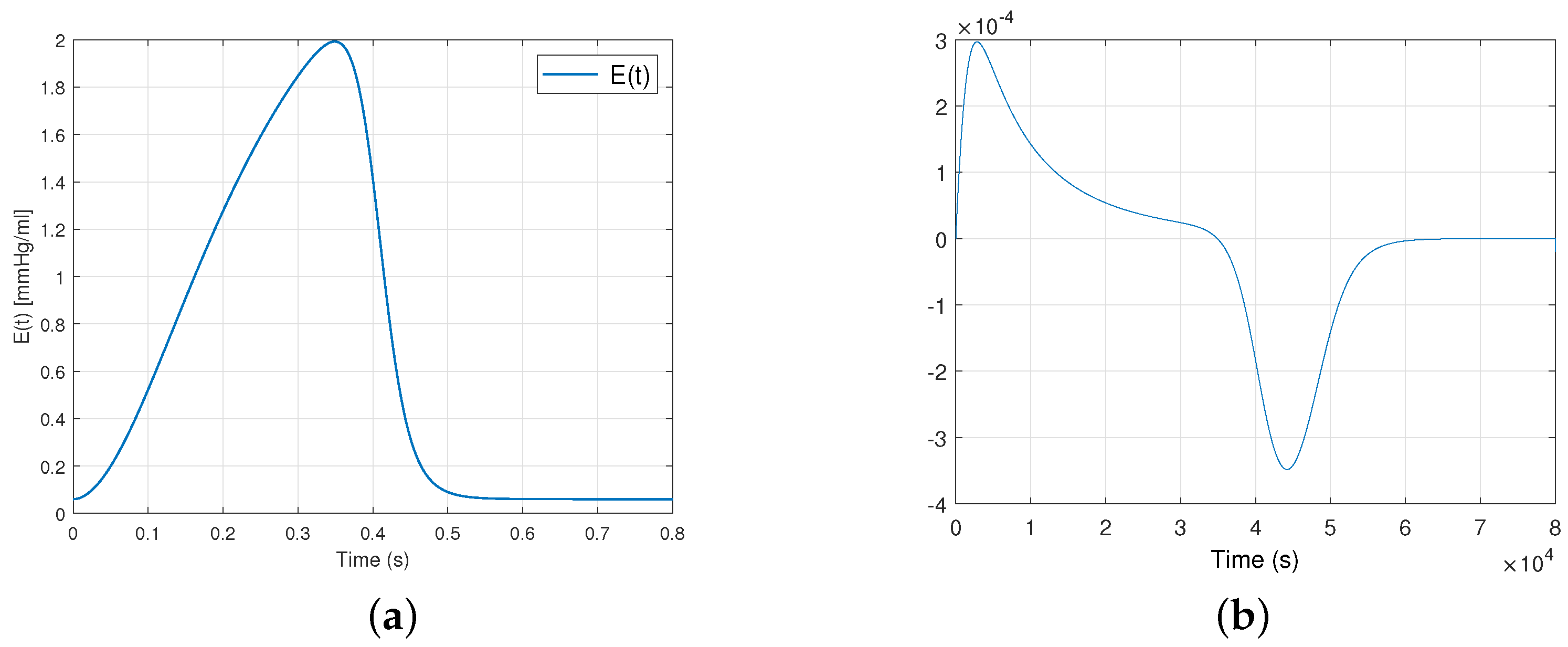
where , with being the heart rate expressed in beats per minute (bpm). The first term within the brackets describes the ascending segment of the curve, while the subsequent term portrays its descending counterpart. The value 1.55 corresponds to the amplitude of elastance, which is associated with the maximum arterial pressure. Additionally, 1.9 and 21.9 indicate the ascending and descending slopes during the LV relaxation period, respectively, while 0.7 and 1.17 are constants that determine the proportional representation of each curve over the cardiac cycle. Figure 3 illustrates the graphical representations of these curves.
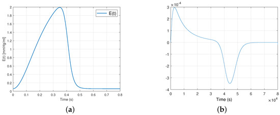
Figure 3.
Plot (a) shows the elastance function and (b) shows the expression for a healthy heart during a single cardiac cycle.
3.3. Presentation of the Mathematical Model of the Cardiovascular System
We consider the CVS model basically given by the following equations [12]:
where represents the state vector of CVS circuit model (see Figure 2 and Table 1 and Table 2) and represents the natural control input sequences of cardiovascular system, with is the state of the mitral valve and is the state of the aortic valve given by:
3.4. Quadratic Normal Form of the CVS [25]
For the remainder of our work of the CVS system, we take the output vector as and the input vector as . Given this output, it is easy to demonstrate that is linearly unobservable in system (4). To proceed with calculating the quadratic normal form, we introduce the following change of coordinates:
which is equivalent to
We directly obtain the quadratic normal form (QNF) [25,26] of the CVS model:
where , , and .
And , , and .
Remark 1.
As a result, building on the work in [25], thanks to the quadratic terms and , we can recover observability for .
3.5. Validation of the Quadratic Normal Form of the CVS Model
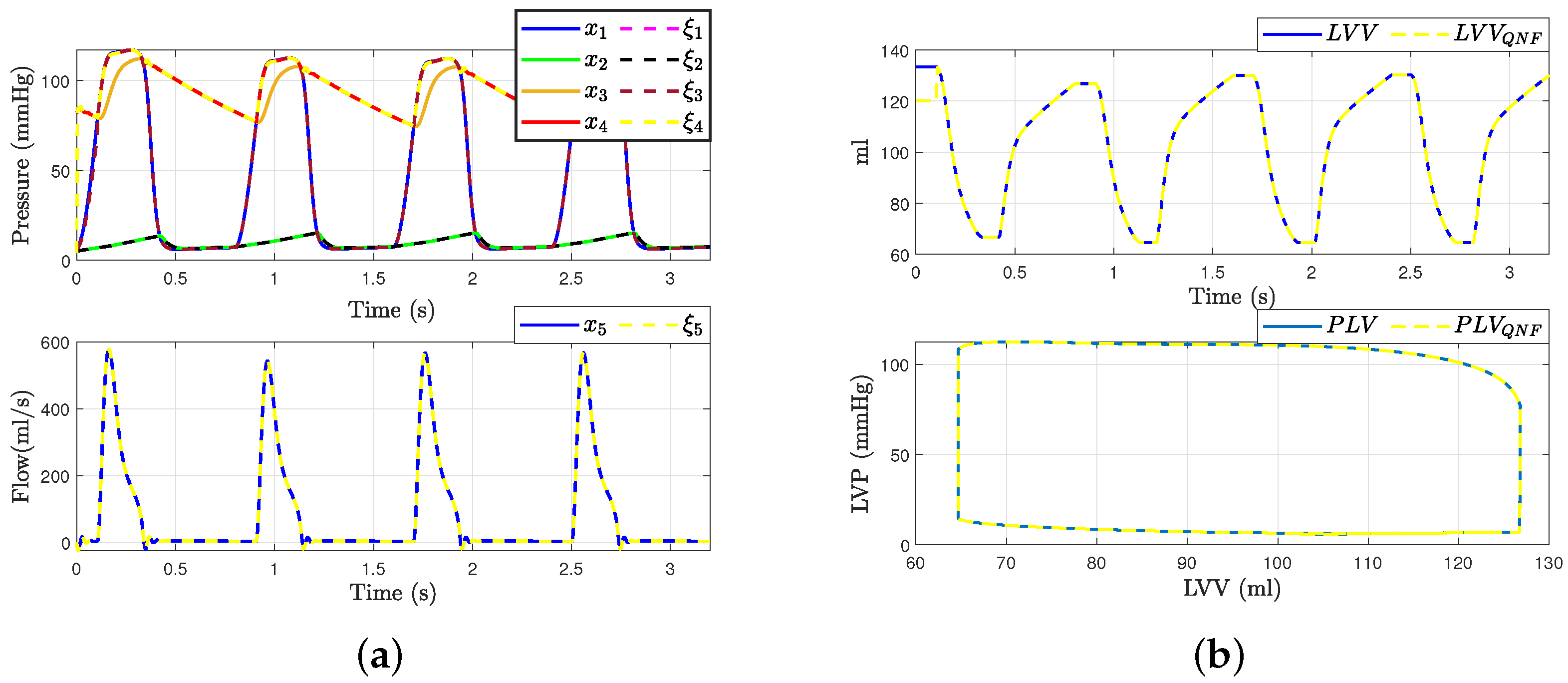
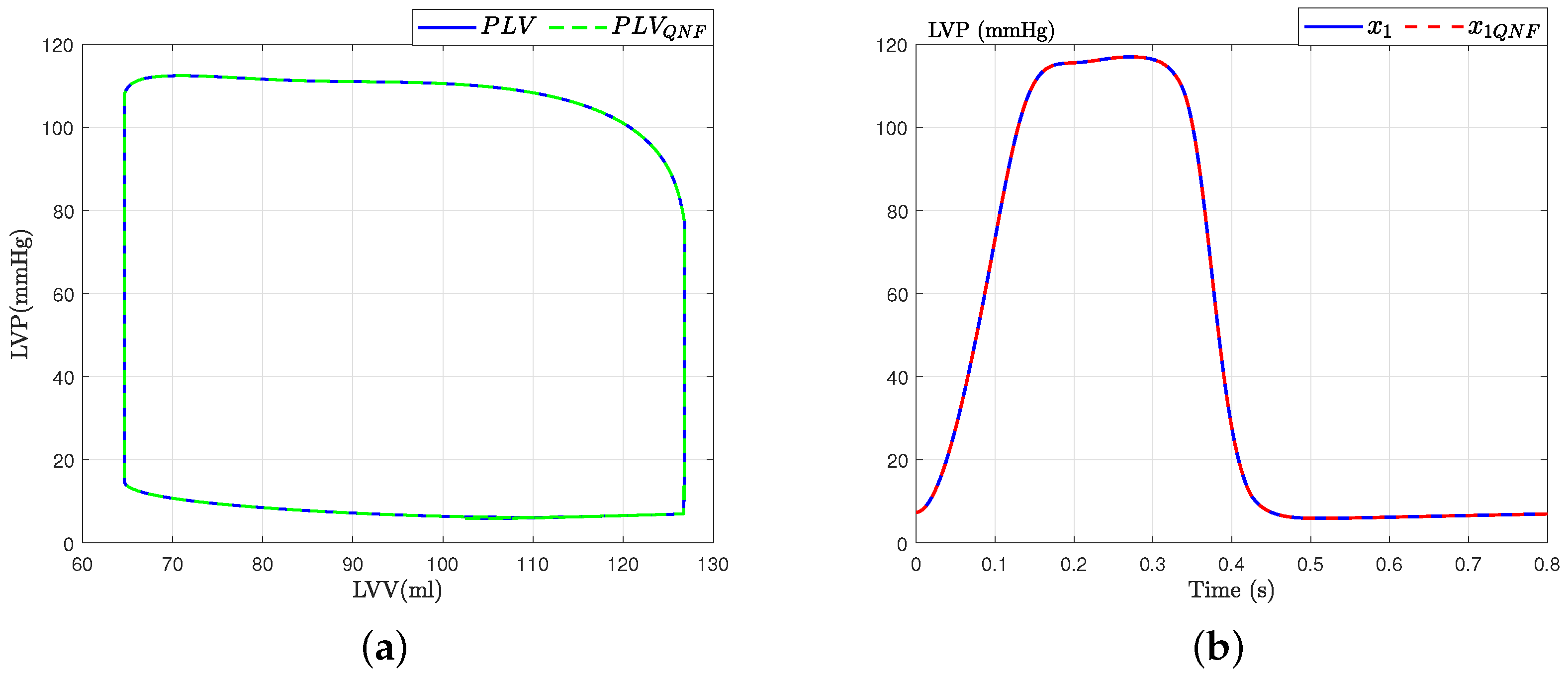
This section presents the validation process for the quadratic normal form of the CVS model obtained, drawing upon previously established validations and incorporating diverse analytical perspectives, as detailed in seminal works such as [6,17]. Initially, the model’s accuracy is substantiated by juxtaposing the waveforms of principal variables, as depicted in Figure 4, against empirical data from healthy subjects reported in [6]. Subsequently, the model’s robustness is assessed through its responsiveness to alterations in preload and afterload factors, ensuring its consistency and reliability in simulating physiological conditions.
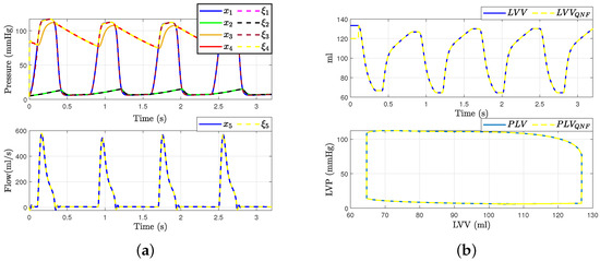
Figure 4.
Hemodynamic waveforms of the CVS model (4) compared with experimental data presented in [6]. (a) Original states and QNF states of CVS; (b) Left ventricular volume (LVV) and preload volume (PLV) in original and QNF system.
With these results, we can affirm that the quadratic normal form obtained offers a novel alternative for the representation of the classical model presented in the literature. Additionally, it is crucial to emphasize that a significant advantage of the quadratic normal form is its capacity to enable the design of observers. These observers can estimate the states of the system that are not directly measurable and apply other control theory concepts. An example of such an application, as discussed in this work, is fault detection and estimation.
The validation of the model also involves a dynamic analysis concerning preload and afterload factors. To evaluate this aspect, we analyze the preload and afterload signals generated by both the original and the quadratic normal form of the CVS model. Figure 5b displays the left ventricular pressure data and the corresponding pressure–volume loop obtained from our model using a volume of mL. It is observed that the dynamics obtained are consistent with those described in [6].
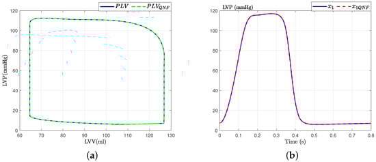
Figure 5.
PV loops for state variable : Left ventricular pressure. (a) PV-loops; (b) Left ventricular pressure.
4. Sliding Mode Observer Design
In this subsection, we will outline the structure of the observer. For a deeper exploration into the design and analysis of observability, readers are encouraged to consult the works cited in [27]. The observer structure presented here accounts for quadratic observability singularities that arise due to state separation or universal input. This methodology is derived from the step-by-step sliding mode approach as detailed in references [28,29,30]. We assume that the states and are directly measurable, but the others are not. The sliding mode observer is described as follows:
In system (9), the auxiliary components are calculated algebraically as follows:
with the following conditions:
If and then otherwise ,
If and then otherwise .
And, to ensure observability is not lost near the observability singularity, you must accurately set and , such that:
If 1 then otherwise , If 1 then otherwise .
Which gives:
Remark 2.
The quality of the estimation of depends on the choice of and . Therefore, it is essential to adjust and within a small neighborhood of the singularity to ensure that the structure without feedback is applied for the minimum amount of time necessary.
Remark 3.
Since and cannot be equal to one at the same time, also , and then when and , we use the quadratic term to recover the information of in this case
and when and , we use the quadratic term to recover the information of in this case
Proof.
The proof of convergence for the observation error is detailed in our article [19]. In it, the stability and convergence analysis of the observer employs equivalent vector methods [31]. The strategy for ensuring the observer’s convergence is implemented step by step across different sliding surfaces. This approach guarantees the convergence of the observation error to zero in three steps and in finite time, in the Lyapunov sense, as further supported by references [19,28,29,30]. □
5. Model for Anomaly Detection
In this section, we will only present the adaptation of the model (8) by including the following fault vector F, which describes the variations affecting the mitral valve and the aortic valve . In the context of the cardiovascular system, variations affecting the mitral valve and the aortic valve are significant contributors to valvular heart diseases, which are a leading cause of cardiovascular morbidity and mortality. We conceptualize the fault in the mitral valve () as the nominal value modeled as a percentile addition or subtraction to the input value (1 or 0) defined in Equation (6). Similarly, the fault in the aortic valve () is considered. Two simple tests were run to evaluate the performance of the proposed FDI methodology: 50% mitral regurgitation, 50% aortic regurgitation. The fault vector is defined by the following equation:
where and are the nominal values of the real state of the mitral and aortic valves, respectively, and are the faults corresponding to the mitral and aortic valves, respectively. The faulty model of the CVS have the following form:
Remark 4.
In observer design, and are considered as bounded unknown inputs [29,30].
The bank of two observers and the residual generator proposed are associated with the SMO designed previously in [19]. In this paper, residual generation is achieved by two single step-by-step sliding mode observers where the faults has been estimated by the observers. In this study, residual generation is obtained through single-step sliding mode observers, which estimate faults and then detect anomalies in the dynamic behavior of the cardiovascular system.
5.1. Residual Generation of Anomalies
The most common valve pathologies are related to the aortic and mitral valves. In both cases, these involve a defect in the closure of the valve, known as valve regurgitation. Aortic valve regurgitation refers to a defect in the valve closure that leads to backward leakage into the left ventricle during diastole. Patients with aortic regurgitation exhibit PV loops with increased amplitude and displacement to the right, indicating that the stroke work is higher, and the pressure–volume area is also increased compared to a healthy case. Similarly, mitral valve pathologies involve leakage during systole from the LV to the left atria (LA).
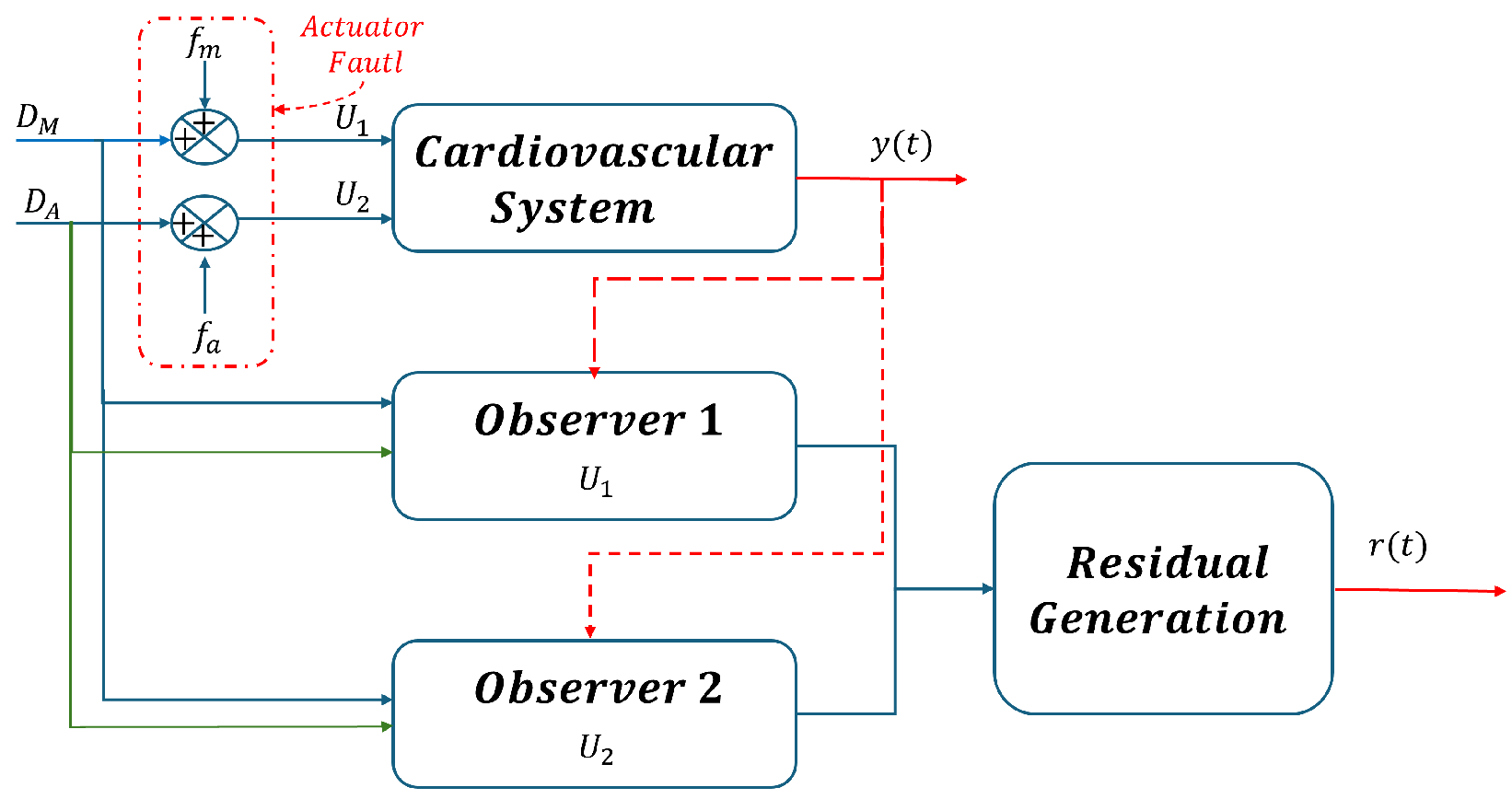
Based on this information, this section presents the design of the fault detection and isolation (FDI) system, this design is based on the assumption that only one fault can occur at any given time. Therefore, two simulation scenarios were considered for fault detection based on the analysis of the generated waveforms pressure. As shown in Figure 6, the first scenario is mitral regurgitation (), and in scenario 2, the fault is aortic regurgitation (). To meet this requirement effectively, the sliding mode observers presented in [19] are used, which enable precise estimation of sensor measurements.

Figure 6.
Bank of observers for all actuator faults estimation.
In Figure 6, the denotes the output vector of CVS, where and . These outputs serve as inputs to the observer, as they are the signals required for the observer to initiate the estimation process.
In this paper, the residuals are defined as the difference between the output variables represents that the most basic residual can be expressed as:
Define as the state estimation error, where
The bank of two observers and the residual generator proposed is associated with the SMO designed previously in [19]. In this paper, the residual generation is achieved by the means of two single step-by-step sliding mode observer, where the faults have been estimated by the observers. When there is no fault, i.e., and , the error will asymptotically converge to the true state. We also observed that the residuals in the presence of an anomaly in the mitral valve are almost the same as the residuals in the aortic valve . However, the changes in the pressure and flow signals of the system are different. This is why, due to the robustness of the observer, we could implement failure isolation and determine when a failure occurs in the mitral and aortic valves.
Below, Table 3 presents a comprehensive signature for residual generation. This table is instrumental in understanding the nuanced differences in residual patterns, which are key to our failure isolation strategy. Each signature has been meticulously derived to ensure the precise detection and localization of anomalies within the mitral and aortic valves, highlighting the sophisticated nature of our observer’s diagnostic capabilities.
Table 3.
Signature for the residual generation.
5.2. Simulation Results
For the initial condition, we refer to those specified in [17], defined as follows:
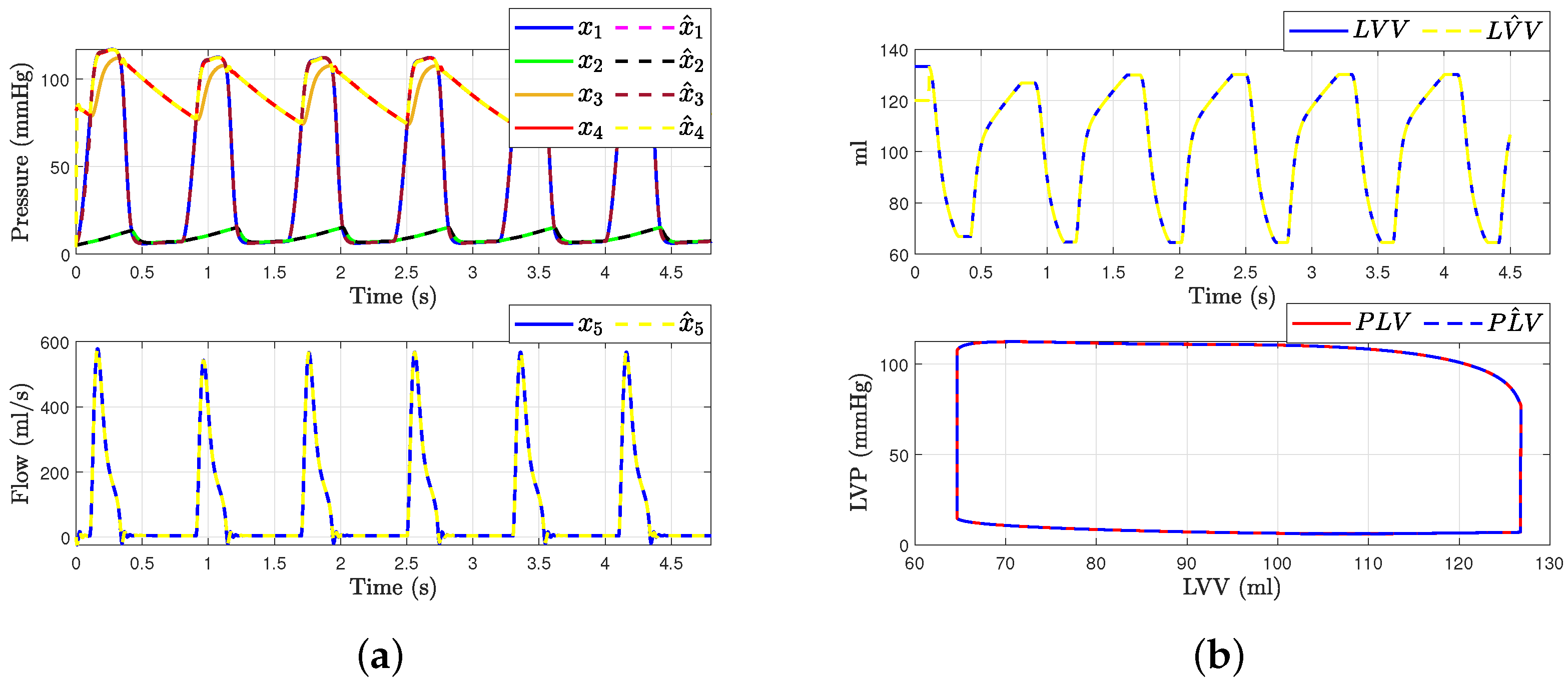
Figure 7 shows the hemodynamic waveforms for a healthy individual with a heart rate (HR) of 75 bpm. The waveforms are consistent, as will be explained. The systolic pressure (LAP) and diastolic pressure (LVP) were measured at 117 mmHg and 77 mmHg, respectively. The ascending aorta pressure (AoP), resulting from the opening and closing of the aortic valve and the pressure wave propagation along the aorta, presented a delayed waveform. From the transformation presented in Equation (1), we can derive the estimated states , , and from the measurable outputs and . Figure 7a presents the states of systems (4) and the observer (9). It demonstrates how the state estimation converges completely for all states within a time frame of 0.2 s.
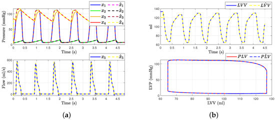
Figure 7.
Hemodynamic waveforms of the CVS model (4) compared with experimental data presented in [6]. (a) shows original states and observer states of CVS for a normal heart and (b) shows left ventricular volume (LVV) and preload volume (PLV) in original and SMO of CVS.
Then, the left ventricle volume and preload volume (LVV) in Figure 7b represent the result of changing afterload conditions. Even with variations in preload and afterload, the relationship between end-systolic pressure and left ventricular volume should be roughly linear if the model functions as predicted. This relationship is known as the end-systolic pressure–volume relationship. By employing an especially built sliding mode observer to estimate the system’s state , we were able to determine the left ventricle’s volume and preload volume using expression (1). This is because the state is described by recalling Frank–Starling’s law, allowing us to gain more insight into the hemodynamic behavior of the heart in a healthy individual. The conditions were simulated with mmHg/mL, = 0.05 mmHg/mL, and = 10 mL.
Remark 5.
These data are compared and confirmed with the results described in [6,7,20], where the aortic pressure and flow waveforms are all consistent with hemodynamics data on healthy individuals.
In the following discussion, two different fault scenarios are presented: Scenario 1 involves mitral regurgitation, while Scenario 2 involves aortic regurgitation.
5.3. Scenario 1: Mitral Regurgitation
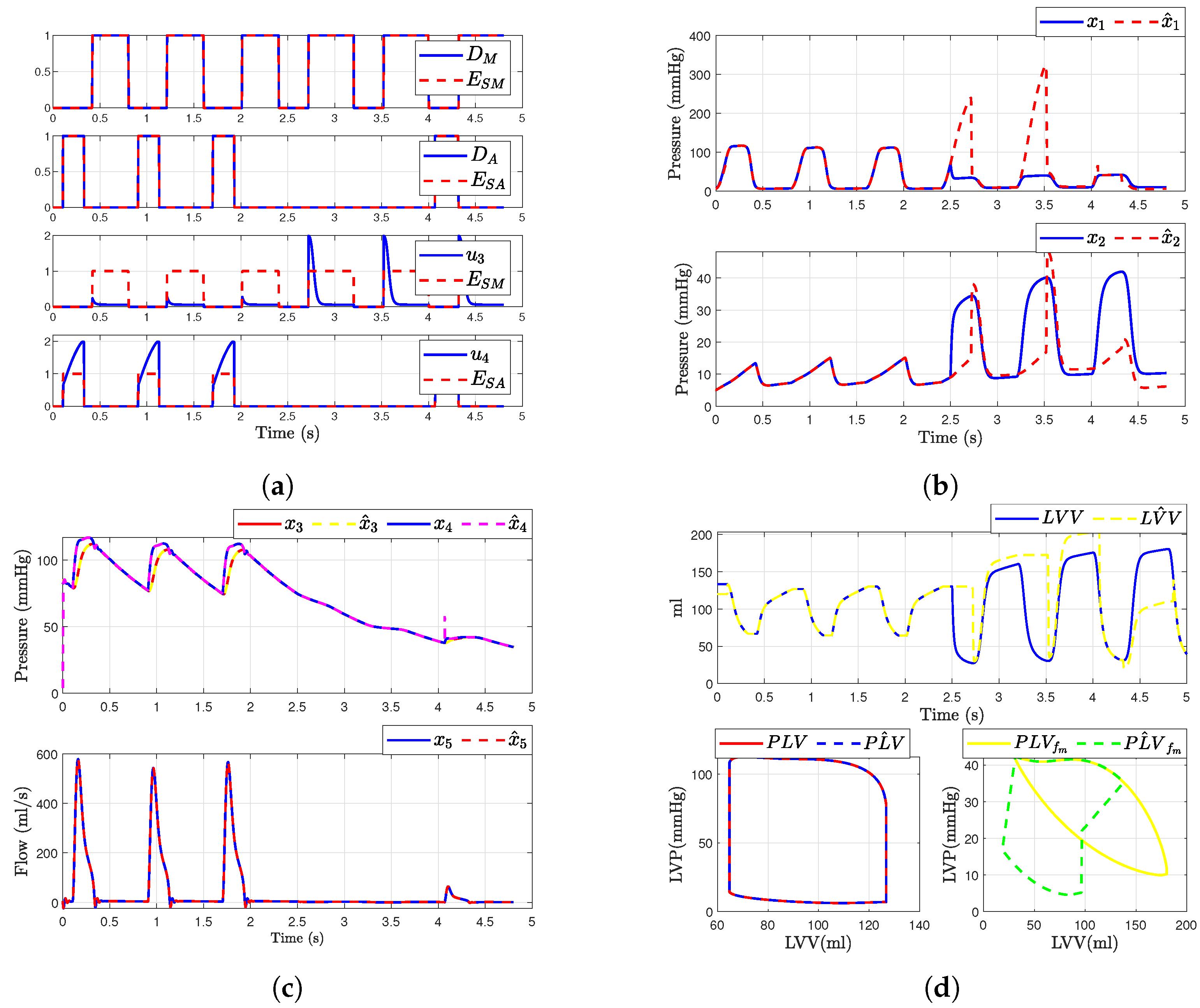
In this scenario, we consider a regurgitation in the mitral valve (i.e., when and ). The simulation of the mitral valve fault was modeled by adding a binary value or to the input . This modification was introduced at time corresponding to the fourth cardiac cycle. Figure 8 illustrates the outcomes following the fault occurrence in the mitral valve. It is observed that, post-fault, the dynamics of the aortic valve, and are altered due to their dependence on and . Figure 8b,c presents the simulated hemodynamic waveforms for an individual with heart failure. The simulation indicates changes in the dynamic system upon fault occurrence, with a decrease in blood flow waveforms and alterations in pressure waveforms.
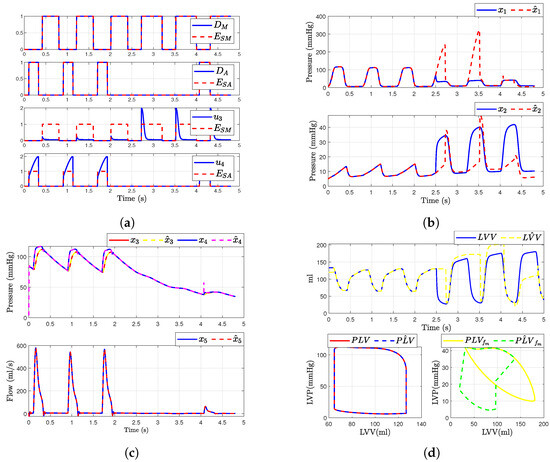
Figure 8.
Simulated hemodynamic waveforms for a failing heart. (a) States of input with fault ; (b) Original states and observer states of CVS for an unhealthy heart ; (c) Original states and observer states of CVS for an unhealthy heart ; (d) Left ventricular volume (LVV) and preload volume (PLV) in original and SMO of CVS.
Additionally, we show that the sliding mode observer can adapt to the change in the system dynamics. The observer can reconstruct the unobservable state when the failure occurs, but only states , , and are able to convergent again to the true state, as shown in Figure 8c. Furthermore, assuming that the heart is healthy, we were able to determine the left ventricular volume and preload volume using the response described by expression (1); providing that the heart is healthy, as shown in Figure 8d. Here is the original model and is the estimated signal provided by the observer (for ). On the other hand, when the failure occurs, the SMO is not able to estimate the volume correctly due to the loss of , as illustrated in the figure showing the failure in the original model and (Figure 8d).
5.4. Case 2: Aortic Regurgitation
In this scenario, we consider a regurgitation in the aortic valve (i.e., when and ). The simulation of fault in the aortic valve was modeled by adding a binary value or to the input . This change was introduced at the time s. Figure 9 represents the results after the fault occurs in the aortic valve. It is evident that, after the fault occurs in the aortic valve, there is also a change in the mitral valve dynamics. Additionally, and exhibit altered dynamics due to their dependence on and . Figure 9 presents the simulation waveforms of the hemodynamics for an individual with aortic regurgitation. We observe changes in the system dynamics when the failure occurs, including variations in blood flow waveforms and an increase in pressure waveforms.
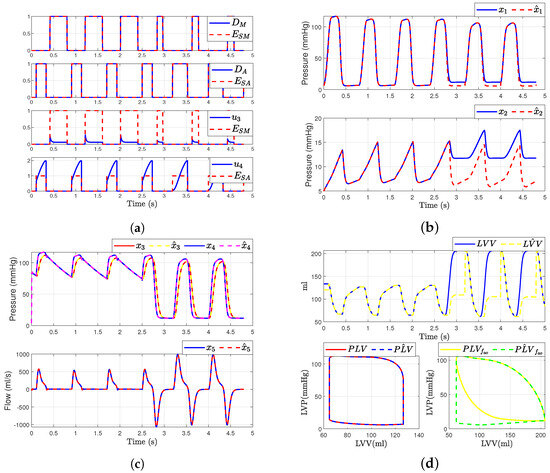
Figure 9.
Simulated hemodynamic waveforms for a failing heart. (a) Input with fault ; (b) Original states and observer states of CVS for an unhealthy heart ; (c) Original states and observer states of CVS for an unhealthy heart ; (d) Left ventricular volume (LVV) and preload volume (PLV) in original and SMO of CVS.
However, we demonstrate that the SMO has the capacity to adapt to the change in in system dynamics. Furthermore, the observer is able to reconstruct the unobservable state when the failure occurs; however, only the states , , and can be convergent again to the true state, while states and have a constant error, as depicted in Figure 9b. Additionally, we were able to determine the left ventricular volume and preload volume using the response described by expression (1), assuming that the heart is healthy, as illustrated in Figure 9d. Here is the original model and is the estimated signal provided by the observer (for ). On the other hand, when a failure occurs, the SMO is unable to accurately estimate the volume due to the loss of , as shown in the comparison between the original model and the observer-estimated model (Figure 9d).
In summary, the results align well with the hemodynamic parameters reported in the existing literature and experimental data, which support the validity of the proposed model and demonstrate its capability to produce results that are comparable to medical data. However, a larger-scale study with a greater number of tests would be necessary to obtain more precise results.
6. Conclusions
This study presents a comprehensive mathematical model of the cardiovascular system capable of simulating both normal and pathological states, specifically focusing on fault detection and isolation. The proposed model, which incorporates electrical analogies, offers a novel representation by transforming the cardiovascular system into a QNF. This form facilitates the design of a sliding mode observer, enhancing the model’s ability to estimate system states and detect anomalies such as valvular heart diseases, which are significant risk factors for cardiovascular diseases.
Our results indicate that the SMO can adapt to changes in system dynamics and reconstruct unobservable states when faults occur. The observer successfully estimated the states , , and , while and showed persistent errors under fault conditions. The model’s validity was affirmed through simulations that replicated hemodynamic parameters that are consistent with the existing literature and experimental data. Additionally, the SMO demonstrated its effectiveness in scenarios of aortic and mitral valve regurgitation by accurately reconstructing the system dynamics post-failure. The results obtained were validated by comparing the data and the simulations presented in [6,7,20].
The findings underscore the potential of the proposed model and observer in clinical decision support, offering a less invasive, economical, and efficient alternative for monitoring cardiovascular health and diagnosing pathologies. However, further studies with larger datasets and a higher number of tests are recommended to refine the model and enhance the precision of the results.
Overall, this work contributes significantly to the field of cardiovascular modeling, providing a robust tool for understanding and managing cardiovascular diseases through advanced fault detection and isolation techniques.
Author Contributions
All co-authors contributed to this work. D.A.S.-C. and L.B.-B. conceived the idea, wrote the original draft, contributed to the investigation and analysis, performed the simulations, edited the manuscript, and contributed to the illustrations. M.D. and C.M.A.-Z. conceived the idea, contributed to the editing and supervised the manuscript. G.V.G.R. provided support in obtaining the data and revised the manuscript. All authors have read and agreed to the published version of the manuscript.
Funding
This research was funded by CONAHCyT, proyect number 320056: Sostenibilidad y Control Automatico.
Data Availability Statement
Experimental data associated with this article will be made available upon request.
Acknowledgments
The authors acknowledge the support provided by CONAHyT and Tecnológico Nacional de México.
Conflicts of Interest
The authors declare no conflicts of interest.
Abbreviations
The following abbreviations are used in this manuscript:
| CVD | Cardiovascular disease |
| WHO | World Health Organization |
| CVS | Cardiovascular system |
| LVP | Left ventricular pressure |
| LV | Left ventricle |
| LVV | Left ventricular volume |
| EDV | End-diastolic volume |
| ESV | End-systolic volume |
| SMO | Sliding mode observer |
| FDI | Fault detection and isolation |
| PV | Pressure–volume |
| PVA | Pressure–volume area |
| LA | Left atria |
| Heart rate | |
| LAP | Left atrial pressure |
| AoP | Ascending aorta pressure |
| F | Total flow |
References
- World Health Organization. Cardiovascular Diseases (CVDs). Available online: https://www.who.int/news-room/fact-sheets/detail/cardiovascular-diseases-(cvds) (accessed on 8 May 2024).
- Chen, C.; Ting, C.-T.; Nussbacher, A.; Nevo, E.; Kass, D.A.; Pak, P.; Wang, S.-P.; Chang, M.; Yin, F.C.P. Validation of carotid artery tonometry as a means of estimating augmentation index of ascending aortic pressure. Hypertension 1996, 27, 168–175. [Google Scholar] [CrossRef]
- Fónod, R.; Krokavec, D. Actuator fault estimation using neuro-sliding mode observers. In Proceedings of the IEEE 16th International Conference on Intelligent Engineering Systems (INES), Lisbon, Portugal, 13–15 June 2012; pp. 405–410. [Google Scholar]
- Ledezma, F.D.; Laleg-Kirati, T.M. Detection of Cardiovascular Anomalies: Hybrid Systems Approach. IFAC Proc. Vol. 2012, 45, 222–227. [Google Scholar] [CrossRef]
- Laleg-Kirati, T.M.; Belkhatir, Z.; Ledezma, F.D. Application of Hybrid Dynamical Theory to the Cardiovascular System. In Hybrid Dynamical Systems; Djemai, M., Defoort, M., Eds.; Springer: Cham, Switzerland, 2015; pp. 315–328. [Google Scholar]
- Traver, J.; Nuevo-Gallardo, C.; Tejado, I.; Fernández-Portales, J.; Ortega-Morán, J.F.; Pagador, J.B.; Vinagre, B.M. Cardiovascular circulatory system and left carotid model: A fractional approach to disease modeling. Fractal Fract. 2022, 6, 64. [Google Scholar] [CrossRef]
- Diaz Ledezma, F.; Laleg-Kirati, T.M. A first approach on fault detection and isolation for cardiovascular anomalies detection. In Proceedings of the 2015 American Control Conference (ACC), Chicago, IL, USA, 1–3 July 2015; pp. 5788–5793. [Google Scholar]
- El Khaloufi, G.; Chaibi, N.; Alaoui, S.; Boumhidi, I.; Driss, E.-J. Design of Observer for Cardiovascular Anomalies Detection: An LMI approach. In Proceedings of the 2022 International Conference on Intelligent Systems and Computer Vision (ISCV), Fez, Morocco, 18–20 May 2022. [Google Scholar]
- Ghasemi, Z.; Jeon, W.; Kim, C.-S.; Gupta, A.; Rajamani, R.; Hahn, J.-O. Observer-based deconvolution of deterministic input in coprime multichannel systems with its application to noninvasive central blood pressure monitoring. J. Dyn. Syst. Meas. Control 2020, 142, 091006. [Google Scholar] [CrossRef] [PubMed]
- Ortiz-Rangel, E.; Guerrero-Ramírez, G.V.; García-Beltrán, C.D.; Guerrero-Lara, M.; Adam-Medina, M.; Astorga-Zaragoza, C.M.; Reyes-Reyes, J.; Posada-Gómez, R. Dynamic modeling and simulation of the human cardiovascular system with PDA. Biomed. Signal Process. Control 2022, 71, 103151. [Google Scholar] [CrossRef]
- Laubscher, R.; van der Merwe, J.; Liebenberg, J.; Herbst, P. Dynamic simulation of aortic valve stenosis using a lumped parameter cardiovascular system model with flow regime dependent valve pressure loss characteristics. Med. Eng. Phys. 2022, 106, 103838. [Google Scholar] [CrossRef] [PubMed]
- Simaan, M.A.; Ferreira, A.; Chen, S.; Antaki, J.F.; Galati, D.G. A dynamical state space representation and performance analysis of a feedback-controlled rotary left ventricular assist device. IEEE Trans. Control. Syst. Technol. 2018, 17, 15–28. [Google Scholar] [CrossRef]
- Ferreira, A.; Chen, S.; Simaan, M.A.; Boston, J.R.; Antaki, J.F. A nonlinear state-space model of a combined cardiovascular system and a rotary pump. In Proceedings of the 44th IEEE Conference on Decision and Control, Seville, Spain, 15 December 2005; pp. 897–902. [Google Scholar]
- Korakianitis, T.; Shi, Y. A concentrated parameter model for the human cardiovascular system including heart valve dynamics and atrioventricular interaction. Med. Eng. Phys. 2006, 28, 613–628. [Google Scholar] [CrossRef] [PubMed]
- Simaan, M.A. Modeling and control of the heart left ventricle supported with a rotary assist device. In Proceedings of the 47th IEEE Conference on Decision and Control, Cancun, Mexico, 9–11 December 2008; pp. 2656–2661. [Google Scholar]
- Astorga-Zaragoza, C. Observer-based monitoring of the cardiovascular system. IEEE Trans. Circuits Syst. II Express Briefs 2019, 67, 501–505. [Google Scholar] [CrossRef]
- Belkhatir, Z.; Laleg-Kirati, T.-M.; Tadjine, M. Residual generator for cardiovascular anomalies detection. In Proceedings of the European Control Conference (ECC), Strasbourg, France, 24–27 June 2014; pp. 1862–1868. [Google Scholar]
- Ramírez-Rasgado, F.; Hernández-González, O.; Astorga-Zaragoza, C.M.; Farza, M.; Barreto-Arenas, O.; Guerrero-Sánchez, M.E. Observer-based supervision of the cardiovascular system with delayed measurements. In Proceedings of the Congreso Nacional de Control Automático, Tuxtla Gutiérrez, Mexico, 12–14 October 2022. [Google Scholar]
- Serrano-Cruz, D.; Boutat-Baddas, L.; Darouach, M.; Zaragoza, C.M.A.; Ramirez, G.V.G. Sliding mode observer design for fault estimation in cardiovascular system. In Proceedings of the Congreso Nacional de Control Automático, Acapulco, Mexico, 25–27 October 2023. [Google Scholar]
- Simaan, M.A. Rotary heart assist devices. In Springer Handbook of Automation; Nof, S., Ed.; Springer: Berlin/Heidelberg, Germany, 2009; pp. 1409–1422. [Google Scholar]
- Mensah, G.A.; Roth, G.A.; Fuster, V. The global burden of cardiovascular diseases and risk factors: 2020 and beyond. J. Am. Coll. Cardiol. 2019, 74, 2529–2532. [Google Scholar] [CrossRef] [PubMed]
- Aluru, J.S.; Barsouk, A.; Saginala, K.; Rawla, P.; Barsouk, A. Valvular heart disease epidemiology. Med. Sci. 2022, 10, 32. [Google Scholar] [CrossRef] [PubMed]
- Hollenberg, S.M. Valvular Heart Disease in Adults: Etiologies, Classification, and Diagnosis. FP Essent. 2017, 457, 11–16. [Google Scholar] [PubMed]
- Manoliu, V. Modeling cardiovascular hemodynamics in a model with nonlinear parameters. In Proceedings of the E-Health and Bioengineering Conference (EHB), Iasi, Romania, 19–21 November 2015; pp. 1–4. [Google Scholar]
- Boutat-Baddas, L.; Boutat, D.; Barbot, J.; Tauleigne, R. Quadratic observability normal form. In Proceedings of the 40th IEEE Conference on Decision and Control (Cat. No.01CH37228), Orlando, FL, USA, 4–7 December 2001; Volume 3, pp. 2942–2947. [Google Scholar]
- Boutat-Baddas, L. Analyse des singularités d’observabilité et de détectabilité: Application à la synchronisation des circuits éléctroniques chaotiques. Ph.D. Thesis, Université de Cergy-Pontoise, Cergy, France, 2002. [Google Scholar]
- Serrano-Cruz, D.A.; Boutat-Baddas, L.; Darouach, M.; Astorga-Zaragoza, C.-M. Observer design for a nonlinear cardiovascular system. In Proceedings of the 9th International Conference on Systems and Control, Caen, France, 24–26 November 2021; pp. 294–299. [Google Scholar]
- Barbot, J.; Boukhobza, T.; Djemai, M. Sliding mode observer for triangular input form. In Proceedings of the 35th IEEE Conference on Decision and Control, Kobe, Japan, 13 December 1996; Volume 2, pp. 1489–1490. [Google Scholar]
- Barbot, J.; Floquet, T. Iterative higher order sliding mode observer for nonlinear systems with unknown inputs. Dyn. Contin. Discret. Impuls. Syst. 2010, 17, 1019–1033. [Google Scholar]
- Floquet, T.; Barbot, J.-P. Super Twisting Algorithm-Based Step-by-Step Sliding Mode Observers for Nonlinear Systems with Unknown Inputs. Int. J. Syst. Sci. 2007, 38, 803–815. [Google Scholar] [CrossRef]
- Draženović, B. The invariance conditions in variable structure systems. Automatica 1969, 5, 287–295. [Google Scholar] [CrossRef]

Disclaimer/Publisher’s Note: The statements, opinions and data contained in all publications are solely those of the individual author(s) and contributor(s) and not of MDPI and/or the editor(s). MDPI and/or the editor(s) disclaim responsibility for any injury to people or property resulting from any ideas, methods, instructions or products referred to in the content. |
© 2024 by the authors. Licensee MDPI, Basel, Switzerland. This article is an open access article distributed under the terms and conditions of the Creative Commons Attribution (CC BY) license (https://creativecommons.org/licenses/by/4.0/).