Abstract
We obtain an accurate analytic approximation for the Bessel function using an improved multipoint quasirational approximation technique (MPQA). This new approximation is valid for all real values of the variable x, with a maximum absolute error of approximately 0.009. These errors have been analyzed in the interval from to , and we have found that the absolute errors for large x decrease logarithmically. The values of x at which the zeros of the exact function and the approximated function occur are also provided, exhibiting very small relative errors. The largest relative error is for the second zero, with , and the relative errors continuously decrease, reaching for the eleventh zero. The procedure to obtain this analytic approximation involves constructing a bridge function that connects the power series with the asymptotic approximation. This is achieved by using rational functions combined with other elementary functions, such as trigonometric and fractional power functions.
1. Introduction
The applications of Bessel functions are common in various fields of science, such as electrodynamics, physics, chemistry, and engineering [1,2,3,4]. As such, accurate approximate analytic functions for and have been obtained recently [5,6]. Furthermore, since integer-order functions are the most significant, we aim to derive a precise analytic approximation for . The same technique, the multipoint quasirational approximation (MPQA) [7], has been applied in previous works but with important improvements for this new function. In the present article, we bridge both the asymptotic expansion and the power series via an analytic approximation. Additionally, we introduce an improvement that may be crucial for future applications. The final approximation combines rational and elementary functions, resulting in a simple function that is easy to calculate with a very low absolute error. Moreover, it provides a very close solution for the zeros of both the exact and approximate functions with a very small relative error. An important aspect of the present approximation is the symmetry preservation, rendering the approximation valid for both negative and positive values of x. This means that the approximate function is constructed as an even function, like the original function , meaning that the same approximation for positive values of x is also valid for negative values. In the initial approximations of [8], this symmetry preservation was not considered, limiting the approximation to positive values of x only. It is important to note that in the Padé method [9,10], power series are used, and the approximation is obtained through rational functions, which are quotients of polynomial functions. In our new technique, asymptotic expansions are as important as the power series. Since these expansions involve additional functions, such as exponential, trigonometric, hyperbolic, and other elementary functions, new types of functions must be used in combination with rational and polynomial functions. This new technique simplifies the approximations and can be applied to all real values of the variable, avoiding the usual restrictions. An additional improvement is to consider the zeros of the function to create new equations for the approximation parameters. The structure of the paper is as follows: First, in Section 2, a detailed description of the method to obtain the new approximation will be presented. The results and errors of the approximation will be discussed in Section 3. The analysis of the zeros of the approximation and relative errors will also be carried out in that section. Finally, Section 4 will be devoted to the conclusion.
2. Theoretical Analysis
The power series of the Bessel function is
and the asymptotic expansion is given by
where , and
These equations are found in many mathematical texts, particularly in Refs. [1,2,3,4]. Considering these series, the approximate analytic function is structured as
In the MPQA technique, the approximation is a quotient of rational functions combined with elementary functions, derived from the asymptotic expansions, which explains the appearance of and . The unusual term here is the radical term , introduced to preserve the symmetries of . The main symmetry is that the function is even in x, starting from the power , which is maintained by and . Furthermore, when x tends to infinity, the asymptotic behavior of Equation (2) approaches . To maintain this symmetry using even powers of x, we use . However, in the numerator, the term “” has the same degree as “”, but the factor x in must be compensated by another term in the denominator, which is now , explaining the term in the denominator. The problem arises with at the end, and thus the term would result in a term with instead of . To avoid this, we use instead of . Consequently, to balance the polynomial terms, we also include . These modifications result in better approximation accuracy.
Now, let us determine the parameters. Three equations are obtained by matching the power series terms of both and . To avoid nonlinear equations, the first step is to rationalize by multiplying by . By identifying the first terms of the expansions in Equations (1) and (4), we obtain
where the initial coefficient 4 arises from , and the power series expansions of , , , and are used:
The following equations are obtained in the zeroth, second, and fourth orders in x:
In the second step, the asymptotic expansion must be considered, and by identifying terms, the following equations are obtained with considered a positive number:
There are five equations, and excluding the parameters , there are six parameters. There are several ways to derive the last equation, for instance, using another term of the power series or the asymptotic expansion. However, we find the best result by imposing coincidence in the first zero of and . Thus, the new additional equation is:
where is the value of the first zero of the Bessel function , that is
The explicit value of is well known to be
considering five digits. The explicit form of Equation (14) is
which can be simplified as
To avoid problems with the so-called “defects” in the Padé method, it is important to impose the condition that q must be positive. The explanation can be expressed as follows: the defects in the Padé technique correspond to one zero in the real axis in the denominator, usually accompanied with a nearby zero in the numerator. In our technique, we use also rational functions as in Padé, but now since all our functions must be even, then our denominator is . If q is negative, zeros in the real axis will be obtained, but if q is positive, the zeros will be complex numbers, out of the real axis. To achieve this, it is convenient to obtain q as a function of . By using the above equations, the result is expressed as
where is given by:
and is given by
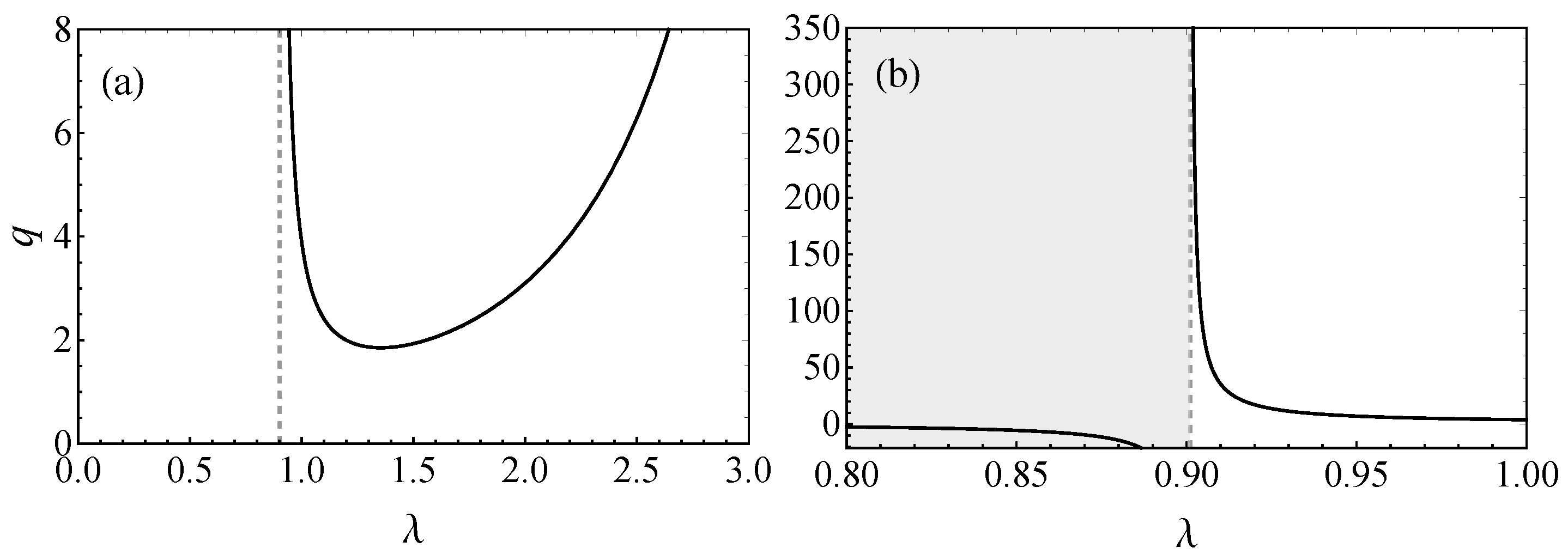
In Figure 1, q is shown as a function of . The optimal is denoted as , which is the value of producing the smallest maximum absolute errors. The procedure is to introduce a value of where q is not negative and to calculate all the parameters of the approximation. Once this is complete, the next step is to determine the maximum absolute error for each . The best will be the one producing the smallest maximum absolute error, which in this case is , yielding a maximum absolute error of for , with a relative error at this point of and .

Figure 1.
The figure in (a) shows the values of wherein , and the one in (b) shows both regions, separated by a vertical line at , and the grey color is where , which is for .
In this work, maximum absolute errors are considered instead of relative ones because the functions have zeros. The errors near the maximum error are now the values of the parameters p and q determined with , and these are shown in Table 1.

Table 1.
Values of parameters of the approximation.
3. Results
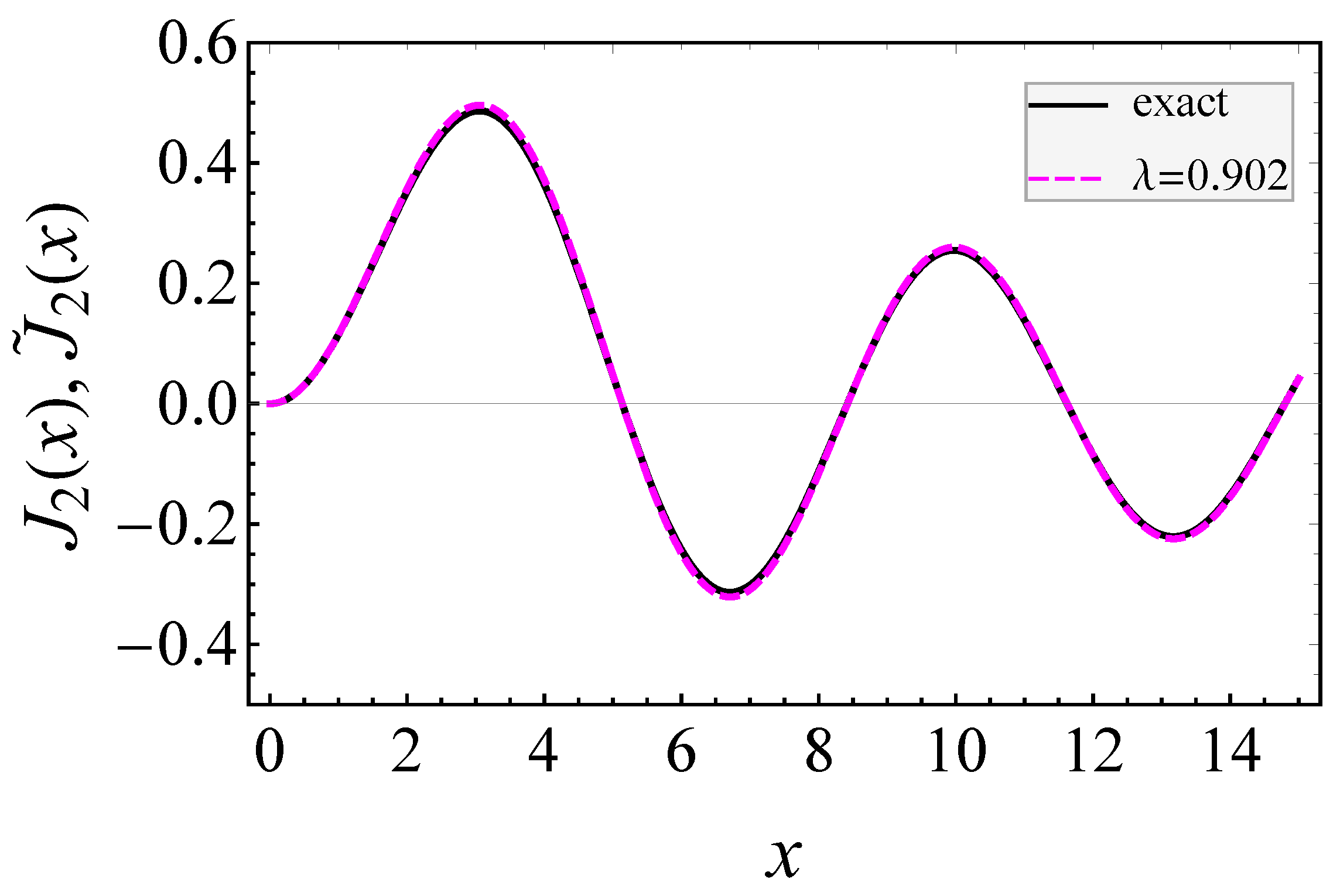
It is noteworthy that a plot of the function and the approximation, on a typical scale, shows only small differences as seen in Figure 2.

Figure 2.
Comparison between the exact function (solid line) and the approximate function (dashed line).
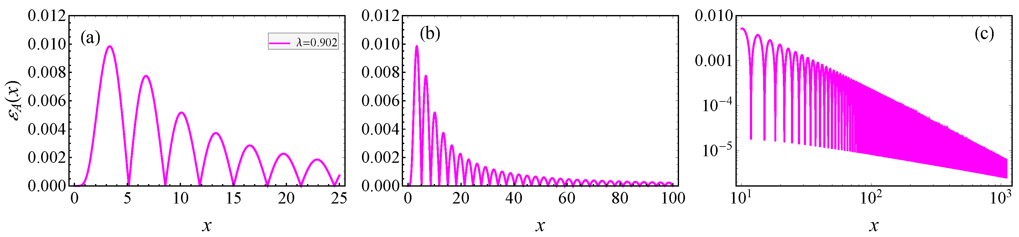
A more interesting result is obtained by plotting the absolute error as a function of the variable x as shown in Figure 3. This figure clearly illustrates that the errors are very small for both small and large values of the variable x. The maximum error occurs at intermediate values. Note that in Figure 3, the range of the variable x in Figure 3b is four times that in Figure 3a, and in Figure 3c the variable is logarithmic as well as the corresponding errors.
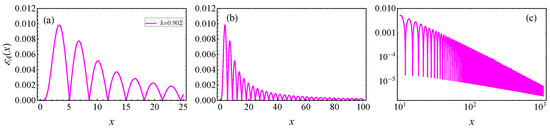
Figure 3.
Absolute errors for . Panels (a) and (b) display from to and to , respectively. Panel (c) displays from to using a logarithmic scale.
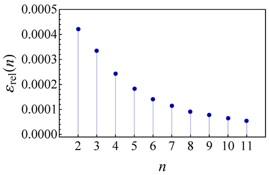
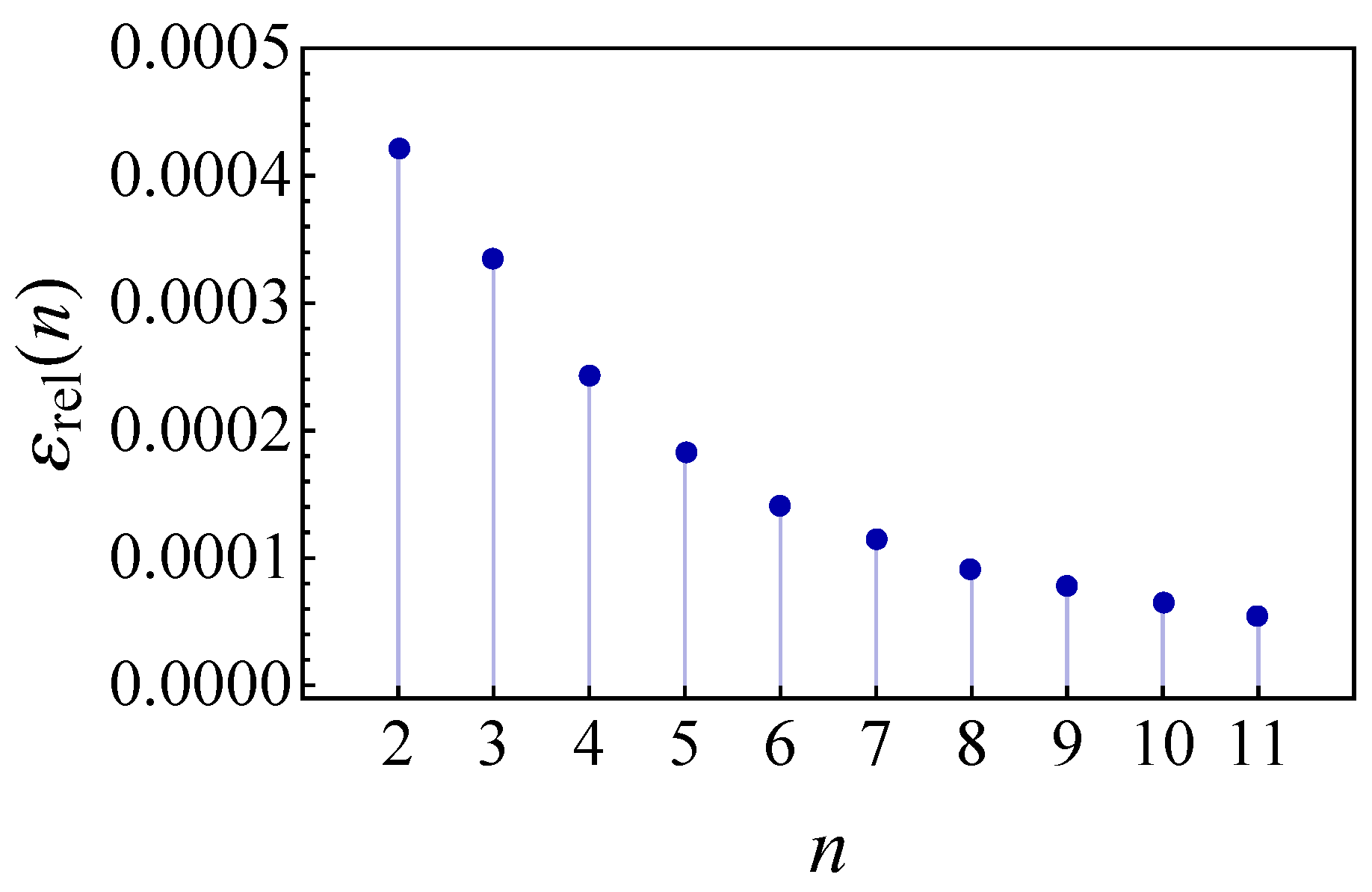
In Table 2, the zeros of the exact function and the approximated function are compared. The first zero is not considered because it coincides with five digits through Equation (17), and each value and is written with only five digits. The relative error of each one, except the first one, is given in the last column of the table. The largest relative error is at the second zero. The formula for the relative error is
where is the n-zero of , and is the corresponding one of . In Figure 4, the relative errors are shown.
Table 2.
Zeros of and .
One important difference between the present technique and the Padé method is that the radius of convergence of the power series is not important for our approximation. The approximations obtained by the present technique are valid for positive and negative values of x since the symmetries are preserved. Another significant point is that the usual problems with the so-called “defects” in the Padé method, which involve a zero in the denominator and another one near the numerator, never appear in the present method. Additionally, by simultaneously using the power series and asymptotic expansions, the relative and absolute errors for small and large values of the variable are minimal, and the largest errors occur at intermediate values of x.
Finally, it is noteworthy that the results obtained are valid for positive and negative values of x, as is an even function as indicated in the paragraph following Equation (4).
We now comment on the comparison between our results with other important approximations previously published, different from the power series and asymptotic expansions already considered. The most notable among these are the so-called polynomial expansions [11,12,13]. These approximations, particularly for , , , and other integer orders, although not specifically for , are derived similarly and yield similar results. These approximations are highly accurate for small values of x, typically for , with errors lower than . However, they fail for larger values of x as demonstrated in Ref. [12]. In contrast, our approximation is valid for all values of x, with the largest error of occurring at an intermediate value of about . Our errors are minimal for small values of x and also for very large values of x (i.e., as ), a characteristic of all approximations using the MPQA technique, which becomes exact for small and large values of the variables as they coincide with the power and asymptotic expansions. Typically, the MPQA method yields good approximations for all positive values of the variable [7]. Moreover, since symmetry is preserved, our approximation is valid for all real values of the variable.
4. Conclusions
A very precise approximation for the Bessel function has been obtained, valid for all real values of the variable x. The method presented here is an improvement on the MPQA technique. In the present method, the structure of the denominator is simpler than in previous approximations for other Bessel functions of the integer order. To obtain the present approximation, both the power series and asymptotic expansion are simultaneously used as is usual in the MPQA method. However, we have improved the method by including an additional approach to derive some of the parameter equations using the zeros of the exact function. The maximum absolute error obtained here is at . However, the errors outside a small interval around this value are much smaller (see Figure 3a), and decreasing logarithmically with x as it is shown in the range from to (see Figure 3c).
It is also noteworthy that the zeros of both and are very close, with the maximum relative error in the position of the zeros being for the second zero. These errors also decrease quickly as it is presented from the second to eleventh zero. Approximations are not usually common in applications of Bessel functions; we believe this is because all previous approximations were for a limited range of the variable. We think that now, with the approximation being valid for all real values of the variable, there is a good possibility that the present approximation could be used in applications where Bessel functions appear in physics and engineering [14,15,16]; see, for instance, Equations (5), (6) and (A1) in Ref. [16], where our results can be considered to give an explicit and analytical expression for .
Author Contributions
Conceptualization, P.M.; all authors contribute equally to the methodology, software, validation, formal analysis, investigation, writing—original draft preparation, writing—review, and editing. All authors have read and agreed to the published version of the manuscript.
Funding
F.C.-P. thanks the University of Antofagasta for the financial support through projects ANT20992 and Semillero SEM18-02. He is also grateful for the ANID-Chile Ph.D. Scholarship number 2023-21230379. J.P.R.-A is grateful for the financial support of FONDECYT Iniciación grant No. 11240637.
Data Availability Statement
The raw data supporting the conclusions of this article will be made available by the authors on request.
Acknowledgments
We thank posthumously the collaboration of the late Fernando Maass, a distinguished scientist and former head of the Physics Department at the University of Antofagasta, Chile. F.C.-P. also acknowledges the partial support as a graduate student in the “Doctorado en Física Mención Física-Matemática” Ph.D. program at the University of Antofagasta. We also thank Nancy Ponzio and Oscar Avalos-Ovando for improving the English of the manuscript.
Conflicts of Interest
The authors declare no conflicts of interest.
References
- Watson, G.N. A Treatise on the Theory of Bessel Functions, 2nd ed.; Cambridge University Press: Cambridge, UK, 1966. [Google Scholar]
- Jackson, J.D. Classical Electrodynamics, 3rd ed.; John Willey and Sons, Inc.: New York, NY, USA, 1998; pp. 111–119. [Google Scholar]
- Khosravian-Arab, H.; Dehghan, M.; Eslahchi, M.R. Generalized Bessel functions. Theory and their applications. Math. Method. Appl. Sci. 2017, 40, 6389–6410. [Google Scholar] [CrossRef]
- Rothwell, E.J. Exponential Approximation of the Bessel Functions I0(x), I1(x), J0(x), J1(x), Y0(x) and H0(x) with Applications to Electromagnetic Scattering, Radiation and Diffraction [EM Programmer’s Notebooks]. IEEE Antennas Propag. Mg. 2009, 51, 138–147. [Google Scholar] [CrossRef]
- Maass, F.; Martin, P.; Olivares, J. Analytic Approximation to the Bessel Function J0(x). Comput. Appl. Math. 2020, 39, 222. [Google Scholar] [CrossRef]
- Maass, F.; Martin, P. Precise analytic approximations for the Bessel function J1(x). Results Phys. 2018, 8, 1234–1238. [Google Scholar] [CrossRef]
- Martin, P.; Castro, E.; Paz, J.L.; De Freitas, A. Multipoint quasi-rational approximations in Quantum Chemistry. In New Developments in Quantum Chemistry; Paz, J.L., Hernandez, J.A., Eds.; Transworld Research Network: Kerala, India, 2009; Chapter 3; pp. 55–76. [Google Scholar]
- Martin, P.; Guerrero, L. Fractional approximations for the Bessel function J0(x). J. Math. Phys. 1985, 26, 705–707. [Google Scholar] [CrossRef]
- Baker, G.A., Jr.; Travers-Morris, P. Padé Approximants; Cambrige University Press: Cambrige, UK, 1996. [Google Scholar]
- Peker, H.A. An Introduction to Padé Approximation. In Current Studies in Basic Sciences, Engineering and Tecnology; ISRES Publishing: Konya, Turkey, 2021; pp. 143–155. [Google Scholar]
- Abramowitz, M.; Stegun, I.A. Handbook of Mathematical Functions; National Bureau of Standards: Washington, DC, USA, 1972; pp. 481–482. [Google Scholar]
- Millane, R.P.; Eads, J.L. Polynomial approximations to Bessel Functions. IEEE Trans. Antenna Propagat. 2003, 51, 1398–1400. [Google Scholar] [CrossRef]
- Li, L.; Li, F.; Gross, F.B. A New Polynomial Approximations for Jv Bessel Functions. Appl. Math. Comp. 2006, 183, 1220–1225. [Google Scholar] [CrossRef]
- Relton, F.E. Applied Bessel Functions; Blackie and Son Limited: London, UK, 1946; pp. 124–151. [Google Scholar]
- Idris, F.A.; Buhari, A.L.; Adamu, T.U. Bessel Functions and Their Applications: Solution to Schrodinger Equation in a Cylindrical Function of the Second Kind and Hankel Functions. Int. J. Novel Res. Phys. Chem. Math. 2016, 3, 17–31. [Google Scholar]
- Eszes, A.; Szabó, Z.S.; Ladányi-Turóczy, B.; Kalácska, I. A Low Side Lobe Level Parabolic Antenna for Meteorological Applications. Prog. Electromagn. Res. Lett. 2024, 115, 91–98. [Google Scholar] [CrossRef]
Disclaimer/Publisher’s Note: The statements, opinions and data contained in all publications are solely those of the individual author(s) and contributor(s) and not of MDPI and/or the editor(s). MDPI and/or the editor(s) disclaim responsibility for any injury to people or property resulting from any ideas, methods, instructions or products referred to in the content. |
© 2024 by the authors. Licensee MDPI, Basel, Switzerland. This article is an open access article distributed under the terms and conditions of the Creative Commons Attribution (CC BY) license (https://creativecommons.org/licenses/by/4.0/).