Enhancing LS-PIE’s Optimal Latent Dimensional Identification: Latent Expansion and Latent Condensation

Abstract

The Latent Space Perspicacity and Interpretation Enhancement (LS-PIE) framework enhances dimensionality reduction methods for linear latent variable models (LVMs). This paper extends LS-PIE by introducing an optimal latent discovery strategy to automate identifying optimal latent dimensions and projections based on user-defined metrics. The latent condensing (LCON) method clusters and condenses an extensive latent space into a compact form. A new approach, latent expansion (LEXP), incrementally increases latent dimensions using a linear LVM to find an optimal compact space. This study compares these methods across multiple datasets, including a simple toy problem, mixed signals, ECG data, and simulated vibrational data. LEXP can accelerate the discovery of optimal latent spaces and may yield different compact spaces from LCON, depending on the LVM. This paper highlights the LS-PIE algorithm’s applications and compares LCON and LEXP in organising, ranking, and scoring latent components akin to principal component analysis or singular value decomposition. This paper shows clear improvements in the interpretability of the resulting latent representations allowing for clearer and more focused analysis.

1. Introduction

The daily application of data science and statistical learning methods warrants automating the discovery of useful latent spaces from linear latent variable models (LVMs). While linear LVMs are often far less complex than large-scale deep neural nets, the latent representations they find can still prove noisy and difficult to interpret, meaning that relationships between variables or which variables are more meaningful in analysis can be hard to find. LVMs can be categorised into reconstruction- and interpretation-centred models [1]. Ironically, these reconstruction-centred models like principal component analysis (PCA) allow for easier interpretation as their latent components are ordered according to the variance explained. Interpretation-centred models, such as Fast Independent Component Analysis (FastICA), attempt to identify interpretable latent presentations (e.g., independent variance contributing sources) but return the latent components unordered. This leads to less interpretable latent spaces, limiting the uptake of ICA in research and industry compared to reconstruction-focused approaches. Independent components (ICs) from FastICA are often noisy and solved sequentially without returning ordered ICs. While this method works well for signal reconstruction, it can lead to single sources spread across multiple ICs, making latent vectors inherently noisy and less interpretable. Figure 1a shows a 3D latent space from which various 2D latent representations can be constructed by projecting the data onto different planes. Different combinations of latent variables lead to more or less structure in the latent space as shown in Figure 1b–d.

This paper extends the optimal latent discovery approaches of the Latent Space Perspicacity and Interpretation Enhancement (LS-PIE) framework. In a previous study [2], we proposed condensing a high-dimensional latent space using latent clustering (LC) into an optimal sub-dimensional latent space, referred to as latent condensing (LCON). In this study, we extend the optimal latent discovery approaches of LS-PIE by proposing latent expansion (LEXP), where we start with a low-dimensional latent space that we gradually expand to an optimal latent space as shown in Figure 2. We successively add latent directions until the explanatory power of the smallest component falls below a user-defined threshold.

For LEXP, at each extension, the total explanatory power of the latent space can be measured, which is iteratively extended, ensuring minimal computation of the latent directions. Depending on the LVM, this approach typically requires less computational time and power than LCON. Both LCON and LEXP can discover optimal latent representations according to user-defined metrics. The proposed extension, LEXP, complements and simplifies the discovery of the latent spaces to enhance their interpretability.

In addition to extending the interpretability of latent spaces by introducing an additional optimal latent discovery approach, this study investigates the similarities and differences between LCON and LEXP on multiple datasets. These include a simple toy problem, complex mixed signals, and two real-world examples in the form of ECG data and simulated vibrational data generated using the SAFE model. In addition, some LVMs such as FastICA split information sources over multiple ICs with an increase in the number of ICs. LCON and LEXP can be used to recover the optimal latent dimensions and directions. This paper improves on the ability of the already proposed methods laid out in the previous paper to generate interpretable components. The simplification of the approach to two methods that utilise the existing methods proposed in the previous paper allows us to analyse and simplify latent spaces with minimal required user input. This allows for the recovery of more optimal representations without requiring time-consuming user-based analysis.

2. Background

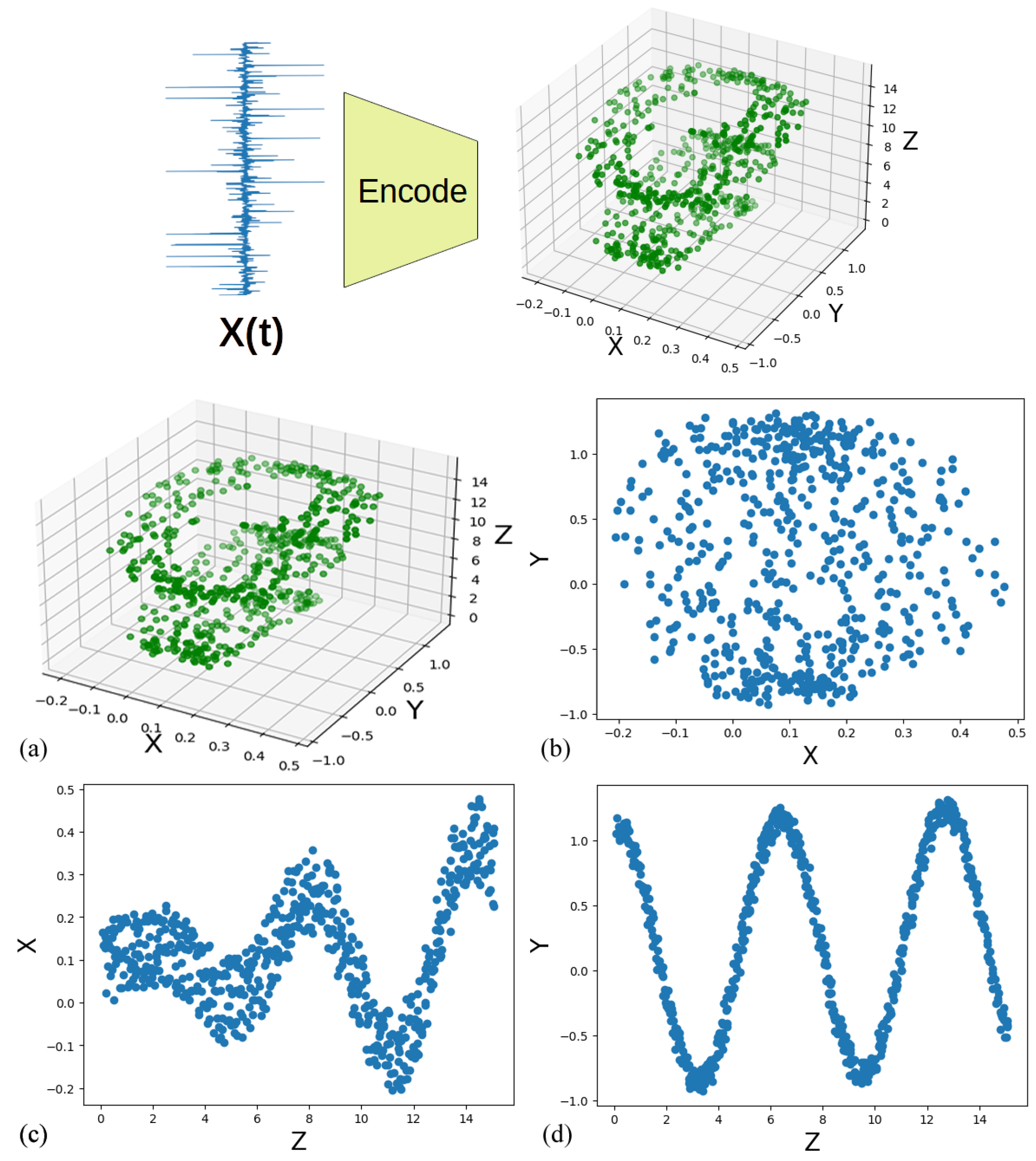
2.1. Latent Spaces

One of the most enduring problems of data science is the “Curse of Dimensionality”, wherein the sparseness of collected data increases exponentially as the number of dimensions increases. This increased sparseness and size of the data space leads to difficulty interpreting results. Many methods have been proposed to extract lower-dimensional representations of higher-dimensional data or latent spaces to counteract this. A latent space, or a latent feature or embedding space, represents compressed data. In this space, items that resemble each other are positioned closer to each other than less similar items. The latent spaces used by latent models are usually of a lower dimension than the original feature space. This is a simple and convenient form of dimensionality reduction [3].

2.2. Latent Vector Models

Many methods can be classified as latent vector models to extract latent spaces. By mapping given data onto a simplified latent space, these models can make predictions, generate new data, and generally simplify the analysis of large datasets. Figure 3 shows the standard structure of LVMs, taking raw training data and compressing it to a latent representation, which can then be sampled to reconstruct the input vector. Once a model has been trained, the latent space can be sampled to generate new data. These latent spaces allow for analysing vast amounts of data in a reduced format while retaining as much information about the dataset as possible. This will enable us to generate interpretable latent space representations of the input data. Two common methods to extract latent spaces are variance-driven PCA and interpretation-driven ICA [4,5,6,7]. Hence, PCA and ICA utilise different independence measures in the latent extraction process [8]. Blind source separation (BSS) is closely related to ICA [9,10]. BSS algorithms allow users to extract useful, statistically independent information from large amounts of mixtures with little or no prior information.

2.2.1. PCA

PCA is a linear dimensionality reduction technique that seeks to find a dataset’s principal components (PCs) using the covariance matrix and maximising the variance. This allows us to extract a lower-dimensional representation of higher-dimensional data while retaining optimal linear reconstructability [7,11]. One of the main features of PCA is the generation of ranked components based on the explained variance of each component. This allows us to calculate the fewest linear latent components for a given reconstruction quality. This means that the extracted latent components are clear in their meaning and easily interpretable, as the variance is often used as a stand-in for explained information, implying that signals with higher variance capture more of the information about the original signal; this means that the sorted components are organised from most to least explained information. PCA is, however, limited in its application in many fields as the algorithm assumes that the data process obeys a Gaussian distribution. In cases where the generative processes are non-Gaussian, methods such as PCA can cause false alarms and therefore, non-Gaussian approaches are needed.

2.2.2. ICA

Independent component analysis (ICA) is a computational method that separates multivariate signals into their additive sub-components. The ICA method of separating a multivariate signal into additive components aims to maximise the statistical independence of these resulting ICs, often using a non-Gaussianity measure as a proxy [6,12,13]. For this reason, it is commonly used as a separation method for mixed signals from multiple sources. This can be seen in its application in solving the “cocktail party problem”, wherein mixed signals from multiple sources are split to extract the source signals. ICA is applied as its maximisation of independence allows for the recovery of statistically distinct signals. It differs from other methods like PCA. In this aspect, PCA aims to maximise the variance rather than a measure of independence [14].

The two main drawbacks of ICA, specifically FastICA, in latent space extraction are the lack of sorting of the ICs and splitting single sources over multiple ICs. This means that the returned ICs are un-ranked and the source information dispersed. This paper proposes a method to generate sorted ICs to put the FastICA algorithm on an equal footing with other linear latent space extraction methods, such as PCA or singular value decomposition (SVD), all of which organise their latent spaces [12].

Methods have been applied to improve the efficiency of the ICA algorithm, such as robustification methods to minimise the effect of outliers. These have included outlier rejection rules and pre-processing steps to improve the separability of the recorded data [15]. Combinations of PCA and ICA have been widely embraced, often using PCA as a pre-processing step for the ICA process. By pre-processing the data using PCA, we transform the data according to the explained variance; this limits our analysis in a way similar to PCA [16].

2.3. Latent Clustering

Clustering methods have been proposed to improve the efficacy of ICA [17]. Methods using Tree-Dependent Component Analysis (TDCA) have been suggested to enhance the classes of dependencies derived by ICA. The TDCA combines graphical models and the Gaussian Stationary contrast function to derive richer dependency classes. A large portion of the focus on ICA and clustering has focused on using ICA in pattern recognition and image classification analysis. Unsupervised methods such as Expectations Maximisation, K-Means, and fuzzy C-Means have all shown satisfactory results when applied to the analysis of MRI imaging. However, these clustering methods are not reliable in terms of accurate classification in pathological analysis [18,19,20]. These methods depend on constructing a similarity graph based on a transformation from a given set X to a set of pairwise distances D or similarities S. Different methods utilise different distance and connection methods to generate different graphs. Different choices of similarity function can lead to the formation of different neighbourhoods and clusterings. For spectral clustering, the local behaviour of these algorithms is more important than the “long-range” behaviours. Therefore, algorithms such as Gaussian Similarity functions can be used.

Similarly, attempts have been made using neural networks to simplify and avoid the local maxima. To adapt the FastICA algorithm to more highly non-linear data, neural networks trained using genetic algorithms have used mutual information maximisation to perform ICA [21].

These methods focus on improving the outputs of the FastICA models, focusing little on the models’ latent spaces.

2.4. Pre-Processing—Hankelisation

A limitation of the FastICA algorithm is the requirement for multidimensional input data. A transformation function is needed to apply the algorithm to single-dimensional time series inputs. From [22], the following method is derived: A single observation of a single channel time series data $\mathbf{x}\in R^{m+n-2}$ can be transformed to enable LVMs to operate on the data [23].

$$\mathit{H}=\left[\begin{array}{ccccc}{x}_0& x_1& x_2& \cdots & x_{n-1}\\ x_1& x_2& x_3& \cdots & x_n\\ x_2& x_3& x_4& \cdots & x_{n+1}\\ ⋮& ⋮& ⋮& \ddots & ⋮\\ x_{m-1}& x_m& x_{m+1}& \cdots & x_{m+n-2}\end{array}\right],$$

This resulting matrix is a symmetric matrix with constant diagonals. This allows for a decomposition of a single-dimensional matrix into multiple shorter signals which can then be clustered. This method has only one variable other than the input signal: the choice of the Hankel window length [18].

3. Materials and Methods

The algorithmic structure of the two optimal latent discovery approaches, LCON and LEXP, is laid out in detail. LS-PIE application is complemented with Hankelisation to increase the dimensionality of lower-dimensional signals and allow for a more in-depth latent analysis. With this addition, the two approaches are showcased in their application to crafted sinusoidal datasets, such as ECG data and SAFE vibrational analysis data.

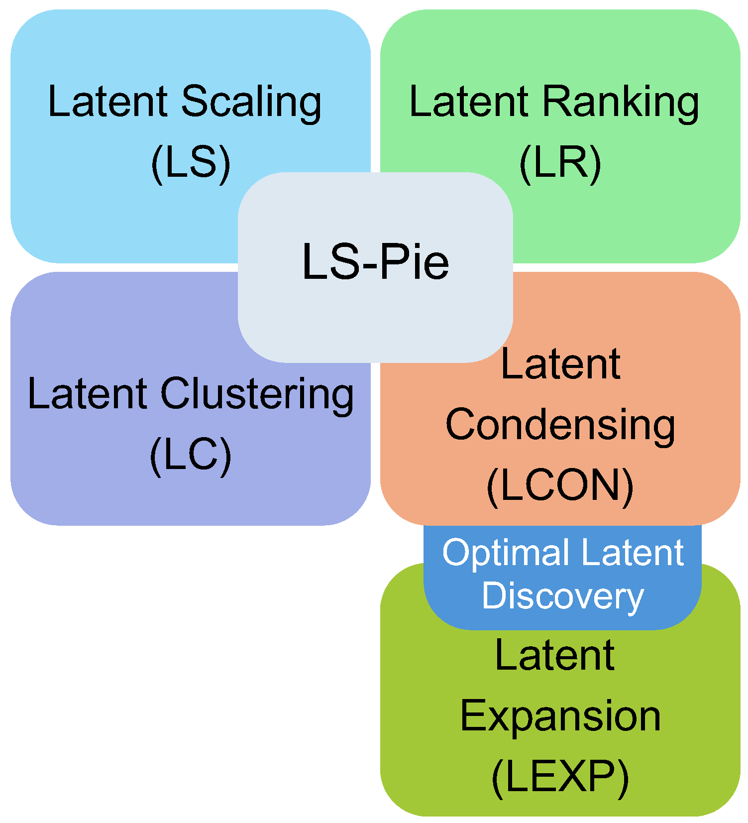
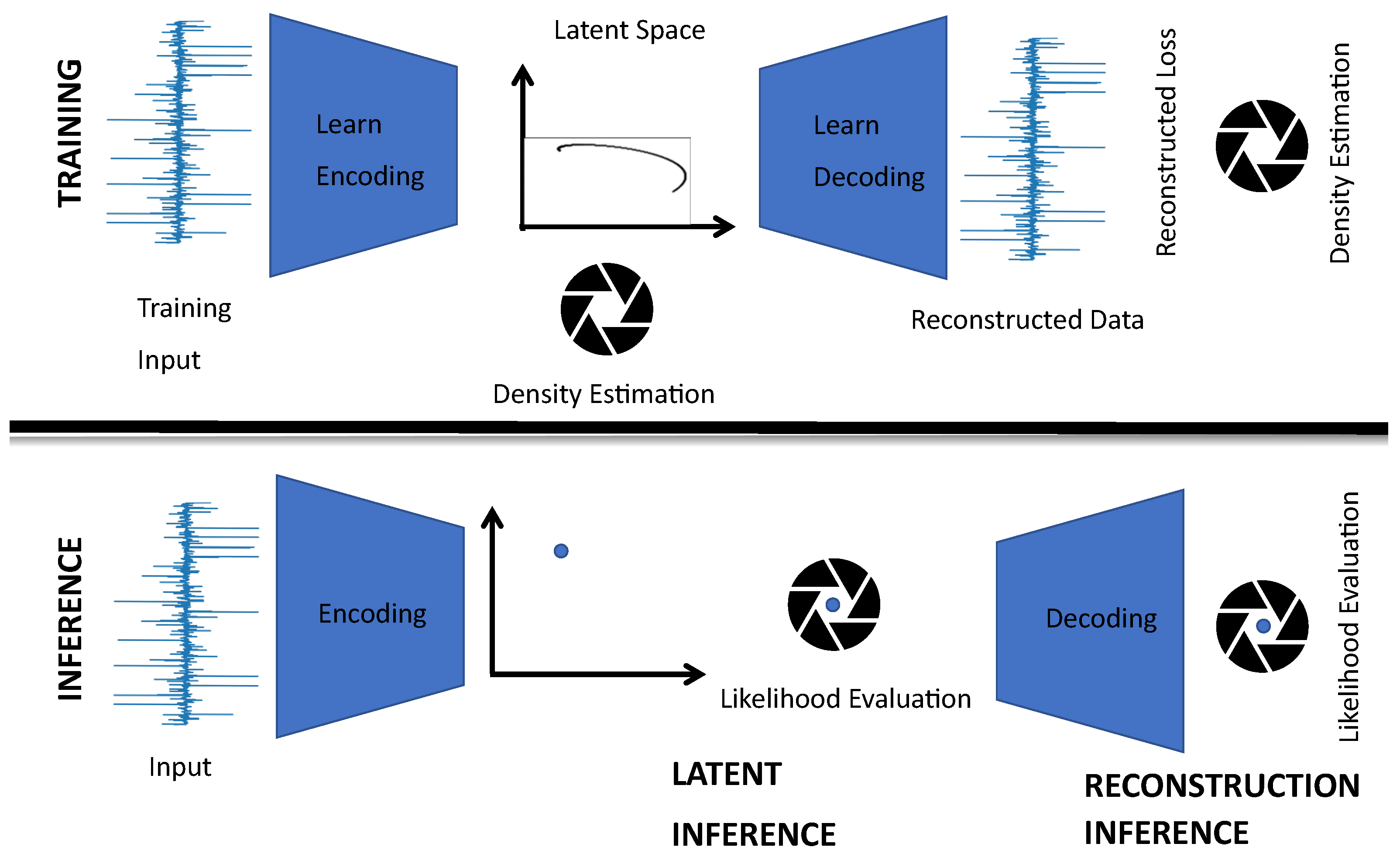
3.1. Optimal Latent Discovery Framework

The main framework for optimal latent discovery is shown in Figure 4, indicating latent condensing (LCON) [2] and latent expansion (LEXP).

In this paper we extend the already proposed LCON method suggested in paper one and we propose the LEXP approach, these two methods allow us to return organised and interpretable latent spaces. By sorting the returned features we can maximise the information contained within minimum features, extending the latent organisation present in PCA to other LVMs as well as allowing for the re-ranking and reorganising of latent spaces according to user preference.

3.2. Optimal Latent Discovery

Optimal latent discovery aims to find the optimal latent space, including its dimensionality, according to a specified user metric. LS-PIE currently supports latent condensing (LCON), as proposed in our previous study [2], briefly discussed in Section 3.2.1. This study proposes a second optimal latent discovery approach, latent expansion (LEXP), as outlined in Section 3.2.2.

These algorithms are designed to be applied to matricised input data. In this paper, we specifically apply the Hankel transform to single-dimensional time series:

$$\mathbf{H}=H\left(\overline{X}\left(t\right)\right)$$

If we already have multi-channel data, as is the case with the heartbeat data, we do not need to pre-transform the data.

$$\mathbf{H}=\mathbf{X}$$

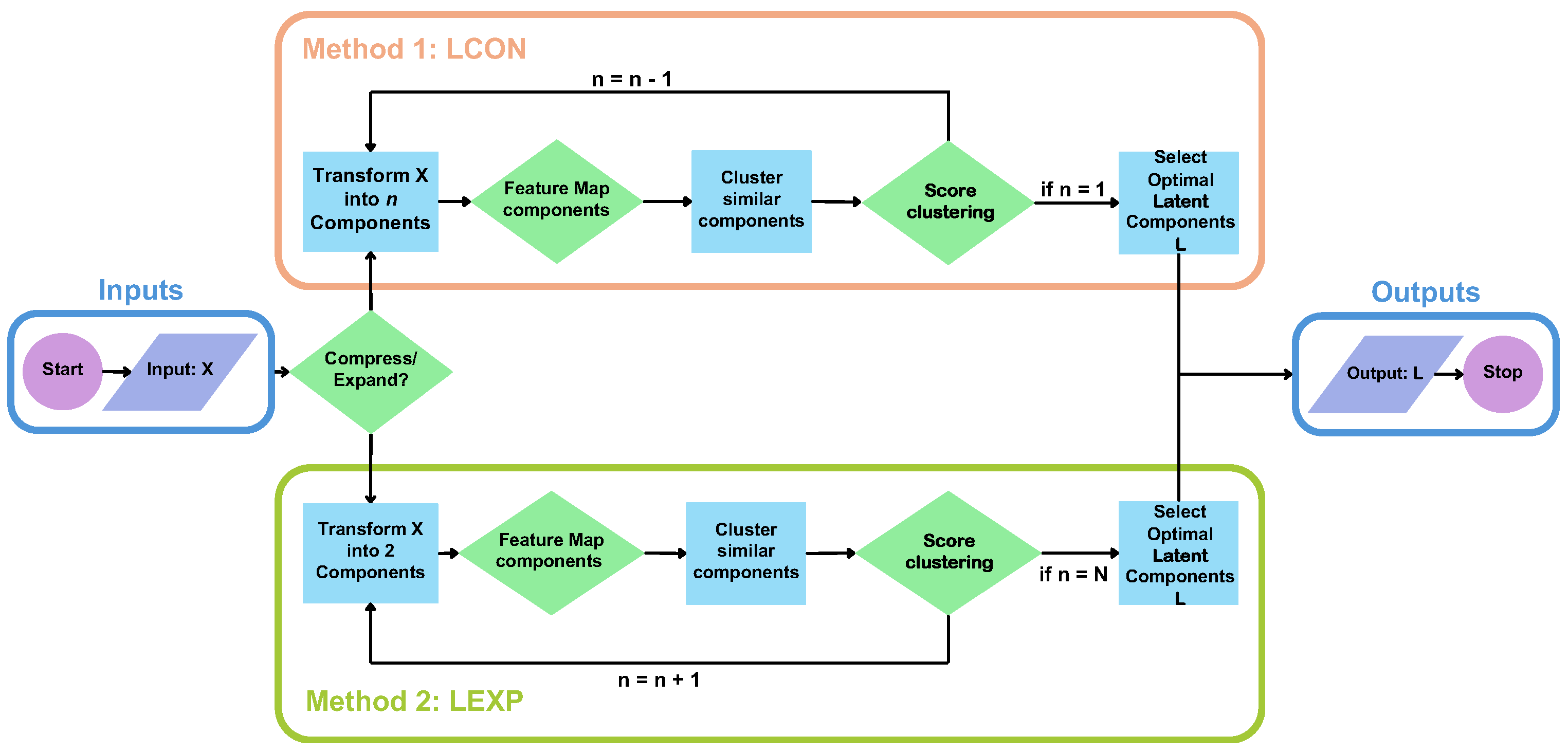
3.2.1. Latent Condensing (LCON)

Latent condensing (LCON) aims to condense a high-dimensional latent space into an optimal-dimensional latent space using a specified user metric. LCON can be achieved using a variety of approaches and for numerous metrics. LCON is conveniently realised using latent clustering (LC). Although LC finds a prescribed number of clusters, LCON automates the cluster dimensionality using one of two main strategies by

• selecting clustering algorithms that find the optimal number of latent clusters such as balanced iterative reducing and clustering using hierarchies (BIRCH) [24,24], density-based spatial clustering of applications with noise (DBSCAN) [25,26], Ordering Points To Identify the Clustering Structure (OPTICS) [27,28], Mean Shift [29] and Affinity Propagation [30,31];
• systematically reducing the latent dimensions and minimising or maximising a selected clustering index to find the optimal number of clusters.

From the algorithm in Algorithm 1, we can see that the method utilises two separate approaches to compressing the latent representation. In both cases, we first transform the data into the maximum number of components using an LVM, in this paper utilising FastICA, and then we map the resulting latent components to a feature space using a feature mapping function, in this case, explained variance. We can then proceed with one of two approaches: The first, the manual approach, decreases the number of components solved for in regular increments, 1 being the most thorough. We can then use the metric to select the optimal number of components from our list.

The second, the automated approach (and the one we utilise in this paper), relies on automatic algorithmic clustering. In this case, selective clustering algorithms can automatically identify the optimal number of latent components. This paper uses the BIRCH and DBSCAN algorithms for this purpose. We utilise our LVMs to resolve the maximum number of components and cluster similar components based on their ranking metric. We can then combine similar components and re-score them to find their final scores/magnitudes.

There are several clustering indexes and approaches that can be used to determine the optimal number of clusters. The Average Silhouette Method (ASM) finds the number of clusters that maximises the average silhouette coefficient [32]. The Elbow Methods (EM) determine the optimal within-cluster sum of squares (WSS) [33]. A gap statistic can be maximised for the total within-cluster variation for different numbers of clusters with their expected values under the null reference distribution of the data [34]. Minimising the Davies–Bouldin Index measures the average similarity ratio of each cluster with the cluster that is most similar to it [35]. Maximising the Calinski–Harabasz Index (CHI), also known as the Variance Ratio Criterion (VRC), measures the ratio of the sum of between-cluster dispersion and within-cluster dispersion [36].

The method proposed in Algorithm 1 is especially effective when applied to methods such as FastICA wherein increased component numbers lead to the splitting of components. However, with these methods, calculating larger numbers of components requires more computational expense.

For methods such as PCA, where successive components are orthogonal, we can very easily compare successive components from the maximally extracted components.

For the course of this paper, we utilise the automatic method within Algorithm 1, maximally decomposing the inputs and then clustering using selected clustering strategies. While this reduces the optimality of the eventual solution, it significantly reduces the computational time. This is due to the unique solutions generated by each iteration of the FastICA algorithm. The application of clustering methods allows for the optimisation of latent condensing.

Algorithm 1 Latent Condensing (LCON) for Hankelised Time Series Data
Require: Hankelised or multi-channel time series data matrix $\mathbf{H}$, latent variable model LVM, clus-tering algorithm C, feature mapping function f, distance metric d, cluster scoring function s, specified or maximum number of latent vectors m, clustering approach $Automatirc$ or not Ensure: Best feature clustering ${\mathbf{R}}_{best}$, cluster score $S_{best}$ and latent components ${\mathbf{L}}_{best}$   1: $S_{best}\leftarrow -\infty$   2: ${\mathbf{R}}_{best}\leftarrow \varnothing$   3: for $k\leftarrow m$ to 1 do
4:     $\mathbf{L}\leftarrow LVM(\mathbf{H},k)$   5:     $\tilde{\mathbf{F}}\leftarrow f\left(\mathbf{L}\right)$   6:     $\mathbf{F}\leftarrow scale\left(\tilde{\mathbf{F}}\right)$   7:     if Automatic then   8:         ${\mathbf{R}}_{auto},{\mathbf{L}}_{auto}\leftarrow C(\mathbf{F},d,\mathbf{L})$	▹ Decompose $\mathbf{H}$ into k latent vectors ▹ Map latent vectors to feature space ▹ User-specified feature space scaling ▹ Automatic feature clustering ${\mathbf{R}}_{auto}$ using user-specified
distance metric d to find protype latent vectors ${\mathbf{L}}_{auto}$
9:         $S_{auto}\leftarrow s({\mathbf{R}}_{auto},{\mathbf{L}}_{auto})$	▹ Cluster scoring
10:         if $S_{auto}>S_{best}$ then 11:            $S_{best}\leftarrow S_{auto}$ 12:            ${\mathbf{R}}_{best}\leftarrow {\mathbf{R}}_{auto}$ 13:            ${\mathbf{L}}_{best}\leftarrow {\mathbf{L}}_{auto}$ 14:         end if 15:     else 16:         for $j\leftarrow k$ to 1 do
17:            ${\mathbf{R}}_j,{\mathbf{L}}_j\leftarrow C(\mathbf{F},d,\mathbf{L})$ 18:            $S_j\leftarrow s({\mathbf{R}}_j,{\mathbf{L}}_j,\mathbf{H})$	▹ Cluster into j clusters using distance metric d ▹ Cluster scoring
19:            if $S_j>S_{best}$ then 20:                $S_{best}\leftarrow S_j$ 21:                ${\mathbf{R}}_{best}\leftarrow {\mathbf{R}}_j$ 22:                ${\mathbf{L}}_{best}\leftarrow {\mathbf{L}}_j$ 23:            end if 24:         end for 25:     end if 26: end for                   return ${\mathbf{R}}_{best}$, $S_{best}$, ${\mathbf{L}}_{best}$
Feature mapping function f:           $f\left(\mathbf{L}\right)=\left[f_i\right]$, where $f_i$ are selected individual feature functions that could include:
0. Identity: $\mathbf{I}\mathbf{L}=\mathbf{L}$	▹ Keeps original vector unchanged
1. Variance: $f_1\left(\mathbf{L}\right)=\left[\mathrm{Var}\left({\mathbf{L}}_{\mathbf{j}}\right)\right],j=1,\cdots ,k$           2. Kurtosis: $f_2\left(\mathbf{L}\right)=\left[\mathrm{Kurt}\left({\mathbf{L}}_j\right)\right],j=1,\cdots ,k$           3. Spectral centroid: $f_3\left(\mathbf{L}\right)={\displaystyle \frac{{\sum }_{j=0}^{N/2}(j·\frac{f_s}{N})·\left|\mathrm{FFT}{\left(\mathbf{L}\right)}_j\right|}{{\sum }_{j=0}^{N/2}\left|\mathrm{FFT}{\left(\mathbf{L}\right)}_j\right|}}$           4. Entropy: $f_4\left(\mathbf{L}\right)=-{\sum }_k{p}_{k}log{p}_k$, where $p_k$ is the probability of the k-th element in ${\mathbf{L}}_j$           Distance metrics d for clustering:           - Euclidean distance: $d(\mathbf{x},\mathbf{y})={\parallel \mathbf{x}-\mathbf{y}\parallel }_2$ [37]           - Manhattan distance: $d(\mathbf{x},\mathbf{y})={\parallel \mathbf{x}-\mathbf{y}\parallel }_1$ [38]           - Cosine distance: $d(\mathbf{x},\mathbf{y})=1-{\displaystyle \frac{\mathbf{x}·\mathbf{y}}{{\parallel \mathbf{x}\parallel }_2{\parallel \mathbf{y}\parallel }_2}}$ [39]           - Mahalanobis distance: $d(\mathbf{x},\mathbf{y})=\sqrt{{(\mathbf{x}-\mathbf{y})}^T{\mathbf{S}}^{-1}(\mathbf{x}-\mathbf{y})}$, where $\mathbf{S}$ is the covariance matrix [40]           Cluster scoring functions s:           1. Silhouette score: $s(\mathbf{R},\mathbf{L},\mathbf{H})={\displaystyle \frac{1}{\left|\mathbf{L}\right|}}{\sum }_{{\mathbf{L}}_j\in \mathbf{L}}{\displaystyle \frac{b\left({\mathbf{L}}_{\mathbf{j}}\right)-a\left({\mathbf{L}}_{\mathbf{j}}\right)}{max(a\left({\mathbf{L}}_{\mathbf{j}}\right),b\left({\mathbf{L}}_{\mathbf{j}}\right))}}$           $a\left({\mathbf{L}}_{\mathbf{j}}\right)$ is the mean intra-cluster distance, and $b\left({\mathbf{L}}_{\mathbf{j}}\right)$ is the mean nearest-cluster distance           2. Variance-based: $s(\mathbf{R},\mathbf{L},\mathbf{H})={\displaystyle \frac{1}{\left|\mathbf{L}\right|}}{\displaystyle \frac{\mathrm{tr}\left({\mathbf{L}}^T{\mathbf{H}}^T\mathbf{H}\mathbf{L}\right)}{\mathrm{tr}\left({\mathbf{H}}^T\mathbf{H}\right)}}$           3. Kurtosis-based: $s(\mathbf{R},\mathbf{L},\mathbf{H})={\displaystyle \frac{1}{\left|\mathbf{L}\right|}}{\sum }_{j=1}^{\left|\mathbf{L}\right|}\left|\mathrm{Kurt}\left({\mathbf{L}}_j^{\mathrm{T}}\mathbf{H}\right)\right|$           4. Frequency-based: $s(\mathbf{R},\mathbf{L},\mathbf{H})={\displaystyle \frac{1}{\left|\mathbf{L}\right|}}{\sum }_{j=1}^{\left|\mathbf{L}\right|}{\displaystyle \frac{{\sum }_k{(f_k-{\mu }_j)}^2\left|\mathrm{FFT}{\left(\left({\mathbf{L}}_j^T\mathbf{H}\right)\right)}_k\right|}{{\sum }_k\left|\mathrm{FFT}{\left(\left({\mathbf{L}}_j^T\mathbf{H}\right)\right)}_k\right|}}$           ${\mu }_j$ is the mean frequency for the j-th latent component

Due to source-based LVMs, such as the FastICA algorithm, each component will be a small fraction of larger sources, which are split to generate more components. These can then be clustered using summative dimensionality methods. In this paper, we apply either the DBSCAN algorithm to extract natural clusters or the BIRCH algorithm to extract a specified number of components. These two clustering methods are applied due to their comprehensive implementations in Python as well as their simplicity of application on datasets; however, any method to reduce the dimensionality of the resulting latent data can be used. The DBSCAN method is used as it does not require a number of components to be specified before application; the BIRCH method is used as it allows for the specification of a number of components as well as being able to handle noise components. The specific metric used to determine component similarity is user specified.

3.2.2. Latent Expansion (LEXP)

The second and, depending on the choice of LVM, less computationally expensive approach, LEXP, to improve linear latent spaces from latent vector models by systematically expanding the latent space. In Algorithm 2, we begin with the fewest possible components and then expand, increasing the dimensionality of our latent space. At each step, we evaluate the latent clusters according to a user-specified metric to ensure we find the optimal latent dimensionality and cluster within it.

Algorithm 2 Latent Expansion (LEXP) for Hankelised Time Series Data
Require: Hankelised or multi-channel time series data matrix $\mathbf{H}$, latent variable model        $LVM$, clustering algorithm C, feature mapping function f, distance metric d, cluster        scoring function s, specified or maximum number of latent vectors m Ensure: Best feature clustering ${\mathbf{R}}_{best}$, cluster score $S_{best}$ and latent components ${\mathbf{L}}_{best}$ 1: $S_{best}\leftarrow -\infty$ 2: ${\mathbf{R}}_{best}\leftarrow \varnothing$ 3: for $k\leftarrow 1$ to m do
4:     $\mathbf{L}\leftarrow LVM(\mathbf{H},k)$ 5:     $\tilde{\mathbf{F}}\leftarrow f\left(\mathbf{L}\right)$ 6:     $\mathbf{F}\leftarrow scale\left(\tilde{\mathbf{F}}\right)$ 7:     for $j\leftarrow 1$ to k do 8:         ${\mathbf{R}}_j,{\mathbf{L}}_j\leftarrow C(\mathbf{F},d,\mathbf{L})$ 9:         $S_j\leftarrow s({\mathbf{R}}_j,{\mathbf{L}}_j,\mathbf{H})$	▹ Decompose $\mathbf{H}$ into k latent vectors ▹ Map latent vectors to feature space ▹ User-specified feature space scaling ▹ Cluster into j clusters using distance metric d ▹ Cluster scoring
10:         if $S_j>S_{best}$ then 11:            $S_{best}\leftarrow S_j$ 12:            ${\mathbf{R}}_{best}\leftarrow {\mathbf{R}}_j$ 13:            ${\mathbf{L}}_{best}\leftarrow {\mathbf{L}}_j$ 14:         end if 15:     end for 16: end for          return ${\mathbf{R}}_{best}$, $S_{best}$, ${\mathbf{L}}_{best}$        Feature mapping function f: See Algorithm 1        Distance metrics d for clustering: See Algorithm 1        Cluster scoring functions s: See Algorithm 1

4. Numerical Analysis

LS-PIE with optimal latent discovery approaches, LCON and LEXP, is showcased for problems. For each problem, we apply both methods. First, we analyse a simple single-channel sinusoidal example problem to compare LCON and LEXP critically. We then analyse multi-channel signals for a foundation cocktail party problem. We consider two experimental datasets where we make the most of the LS-PIE module’s rank functionality. A real-life medical heartbeat data to demonstrate LS-PIE’s applicability to actual signal separation problems. To conclude, we consider SAFE-guided wave data to showcase the practicality of simplifying data representations and improving latent analysis.

4.1. Datasets Overview

4.1.1. Foundational Problem: Single-Channel

To show the effects of the LS-PIE module on the generated latent spaces, we consider a foundational example f$\left(t\right)=sin\left(2\pi t\right)$, uniformly sampled at ${\displaystyle \frac{4000}{12\pi }}$ samples per second using Hankelisation with a window length of 300. In turn, Figure 5(right) is a signal with decreasing frequency over time, expressed by $f\left(t\right)=sin\left(2\pi t^{0.85}\right)$.

4.1.2. Foundational Problem: Complex Mixed Signal

One of the main applications of source-based LVMs is extracting component sources from mixed signals. This is the classic “Cocktail Party Problem”, wherein the data are generated by mixing periodic signals and random noise. This is one of the foundational problems to which the FastICA can be applied to extract the component signals. In this case, a combination of sinusoids, square signals, and saw-tooth signals are used [41].

4.1.3. Experimental Data: ECG Heartbeat Categorisation

To showcase the application of the module to real-world, multi-channel data, we apply the module to a compiled ECG Heartbeat Categorisation Dataset. This dataset consists of 14,552 samples at 125 Hz fall within two categories: healthy and unhealthy.

This dataset has been used to train deep neural networks [42]. However, each of these samples is of a very high dimension, consisting of 188 data points requiring larger deep neural networks to analyse.

These data are available through PhysioNet as a combination of the MIT-BIH Arrhythmia Database and the PTB Diagnostic ECG Database. Optimal latent discovery is applied to examine the scores of the outputted components rather than the components themselves, as we wish to demonstrate the effect of an increasing component number on source-based LVMs like ICA compared to variance-based methods such as PCA.

4.1.4. Experimental Data: Vibration Guided Wave-Based Monitoring

Accurate guided wave system monitoring relies on precisely understanding mode propagation characteristics.

In this case, sets of material and geometric attributes were provided to a Semi-Analytical Finite Element (SAFE) model, with each observation generated considering a rail with uniform material properties described by a density, an elastic modulus, and a Poisson’s ratio [43]. The time series data are transformed into dispersion curves for the various isolated propagating modes [44]. These dispersion curves are scaled to cover a range of longitudinal speeds of sound of the rail material. This allows us to test the multi-channel methods on a variety of problems. The resulting dispersion curves can be hard to analyse as they are complex and highly non-linear. Finding lower-dimensional representations of these data simplifies the analysis of rail systems and allows for greater interpretability of both the SAFE models and the measured rail data [43,45].

4.2. Optimal Latent Discovery: Single Channel

For each of the single-channel signals, Hankelisation was used to increase the dimensionality of the data using a window length of 400. The data did not require normalisation. In this section, we show the resulting analysis using eight latent variables using PCA and ICA in Figure 5(left). Here, we expect identical results for PCA and ICA, merely a single-frequency Fourier sine–cosine decomposition as shown in Figure 6. Note the improvement in informativeness as LEXP is applied. In turn, note the improvement in the informativeness of the latent directions of LEXP and enhancement of LCON on ICA. For ICA, LCON combined the second- and third-ranked ICs. Here, we expect to see some differentiation in the latent directions between PCA and ICA, as shown in Figure 7. The improvement in the interpretation and informativeness of the latent directions using LS-PIE is evident. LS-PIE isolates and enhances the essential latent directions, which allows time for a critical interpretation of the latent directions and a comparison between LVMs.

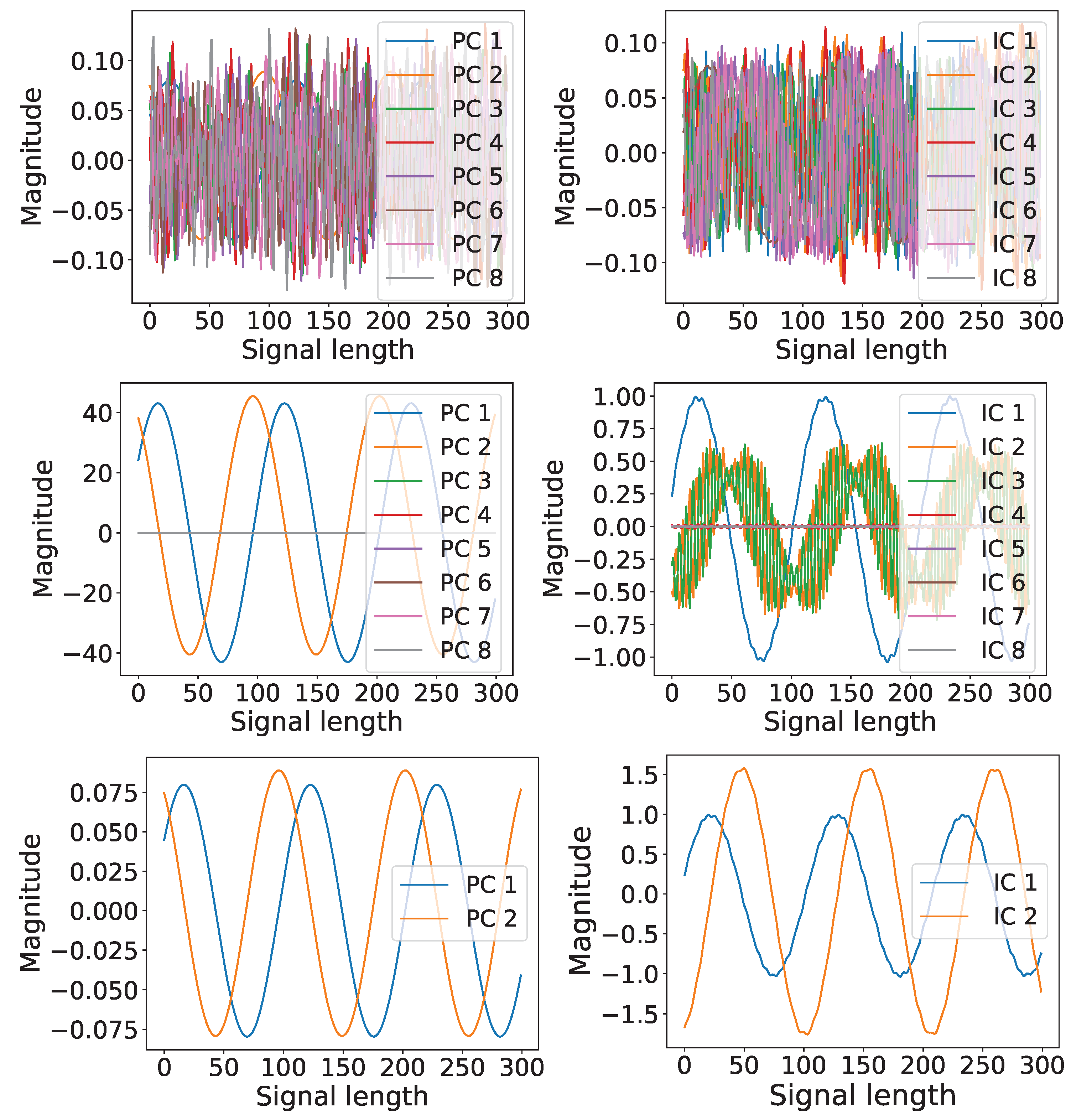
4.3. Optimal Latent Discovery: Complex Mixed Signals

The complex mixed signals did not require Hankelisation as a pre-processing step. In this case, the mean-centred, normalised data were used as an input to the LVMs applied.

While these methods are effective for analysing lower-dimensional mixed signals, we can also generate simulated examples with higher-dimensional mixed signals, as illustrated in Figure 8. By comparing the sorted and unsorted ICA in this figure, it is evident that ICA outperforms PCA in source separation or recovering mixed signals. Specifically, the LS-PIE-augmented FastICA method returns a scaled version of the input signals, successfully recovering the unmixed components. In contrast, PCA only extracts the largest single signal, flattening the rest of the mixed inputs. In this case, the application of LEXP allows us to recover a similar shape to the unsorted inputs.

We can also apply LCON to this problem using two clustering methods. In the first case, we can see in Figure 9 where we apply clustering to the data but allow it to recover the number of input signals. In this case, we recover very similar results to those of the LEXP due to the data’s limited dimensionality. However, in this case, the processed data do not match up as neatly to the original signals.

We can also apply LCON, allowing the cluster method to extract the number of components. This can be seen in Figure 10. In this case, we allow the DBSCAN algorithm to compress the latent space to one component maximally. This reduces the information as we cover only one signal; however, we can see that it acts as an approximation of all 10 input signals.

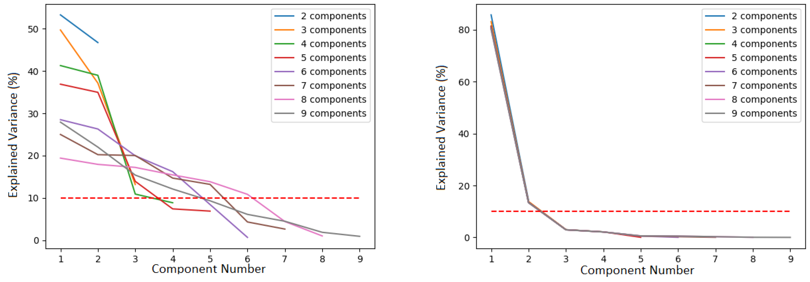
Comparison: Impact of Increasing Number of Components

From Figure 11, we can see the potential of automating the process of LS-PIE for some cutoff metric. In this case, if we choose an explained variance of less than 10% for the least informative component, we can see that this component is found for $n_{components}=3$. However, if we increase the number of solved components, the information in existing components drops. This contrasts with the solution found by variance-driven methods such as PCA, for which the explained variance per component is independent of the total number of components found.

This showcases a classic flaw with source-based LVMs, which can be countered by the combination of LS-PIE and automation, ensuring that sources are not overly decomposed.

4.4. Experimental Datasets: Heartbeat Data

The ECG data did not require Hankelisation as a pre-processing step as the signals were already multi-channel. In this case, the mean centring and normalisation were applied to the data before they were input to the LVMs. First, we apply LS-PIE-enhanced LVMs to normal and abnormal heartbeat sets. For this example, Hankelisation was not required, as each input sample could be taken as a channel, allowing us to rank/cluster without transforming. This would allow us to compress the dataset from 10,000+ signals sampled at 125 Hz into 10,000+ signals consisting of a limited number of predetermined components, in this case, three and four, respectively. The increased complexity of the abnormal heartbeat data leads to the generation of additional components.

This is shown in Figure 12. Here, we can see a distinct difference between the two sets, with normal heartbeats returning one large component and two smaller ones. At the same time, the unhealthy data generate two larger and two smaller components. This distinct difference means that the latent scaling algorithm should be able to function as pre-processing for classification. Hankelisation was not required in this case, as each input sample could be taken as a channel.

From Figure 13, we can see that the clustering functionality overly compensates for the noise in the data, gathering all meaningful information into a single signal while returning two noise signals. This means that the statistically significant distribution generated by the ranked LS-PIE functionality is absent in the clustered signals.

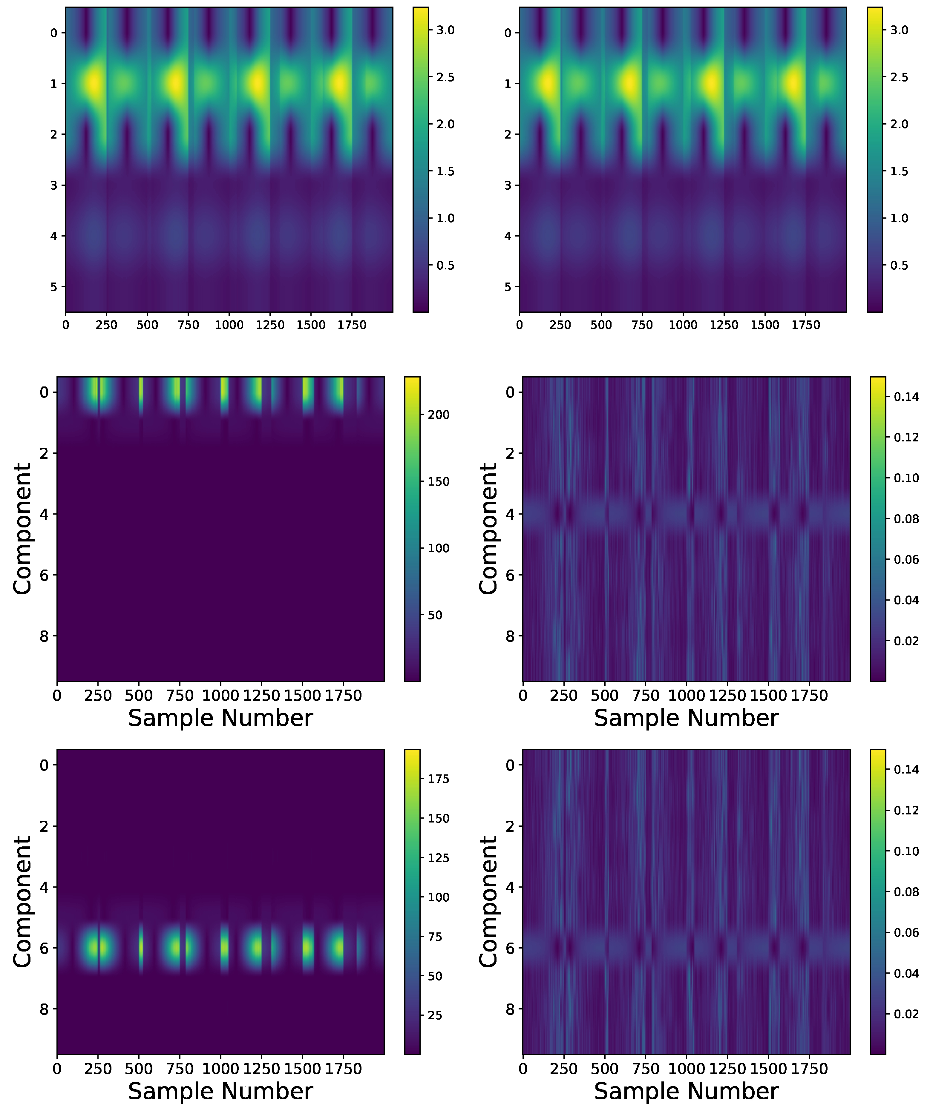
Comparison: LCON and LEXP

This section clearly shows the improvements added using the LS-PIE functionality to improve the analysis of large datasets. From Figure 14, we can see an even clearer representation in the difference between LCON and LEXP. In the case of noisy, less linear data, the ranking functionality was able to separate clear differences in magnitude between the two data types, whereas the clustered method overcompensated, forcing all the information into one meaningless vector. However, both of these contain more information than undirected FastICA decomposition; in this case, the components were over-decomposed, and the information was lost to random noise.

4.5. Experimental Data: Vibration Guided Wave-Based Monitoring

In this section, we compare the breakdown of three separate input modes; each of these three cases consists of a choice of one of the modes generated by the SAFE model.

This model generates randomised samples that fall into a set of mode shapes, as shown in Figure 15. In this case, we sample example signals from three of the mode shapes; each of these samples is then normalised using the mode’s mean.

The SAFE data did not require Hankelisation as a pre-processing step as the signals were already multi-channel; however, the Householder transform was applied to the data first to recover multi-dimensional latent representations. In this case, the mean centring and normalisation were applied to the data before they were used as input to the LVMs.

By ranking the outputs, we can minimise the number of components. This ensures that the information contained within each source is maintained.

The examples show that the ranked LS-PIE-augmented components do not decay as quickly as the PCA results and retain less noise than the initial Eigenvalue decompositions. In Figure 16, we can see that the FastICA decompositions spread their explained variance across components, whereas PCA and Eigenvalue decomposition, with their inbuilt ranking systems, concentrate the variance in the first component. In both of these methods, noise from the normalisation is reflected in the extracted components. This is especially clear in Figure 17; in the latter case, we can see that the primary component extracted in both cases is influenced by the normalisation noise and the curvature of the shape. By ranking the extracted ICs, we managed to avoid noise-based distortion.

We can also apply the LCON approach to the decomposed signals. In this case, we run into complications due to the higher dimensionality and non-linearity of the input. Applying the clustering algorithm to the same dataset in Figure 18, we can see that the initial clustered component matches the first Eigenvector almost exactly. However, the non-linearity decomposes where we only have a single “source” that accounts for all the variance across the data. This showcases one of the foremost issues in using linear decomposition methods to analyse non-linear data. We find increasingly similar sources as we further increase the number of sources to be solved. These are clustered into a single source containing maximal information and a noise source. This can be seen in Figure 18. However, when we examine Figure 19, we can see that, in the cases of both PCA and Eigenvalue decomposition, a single maximally informative source is recovered that explains almost 100% of the variance.

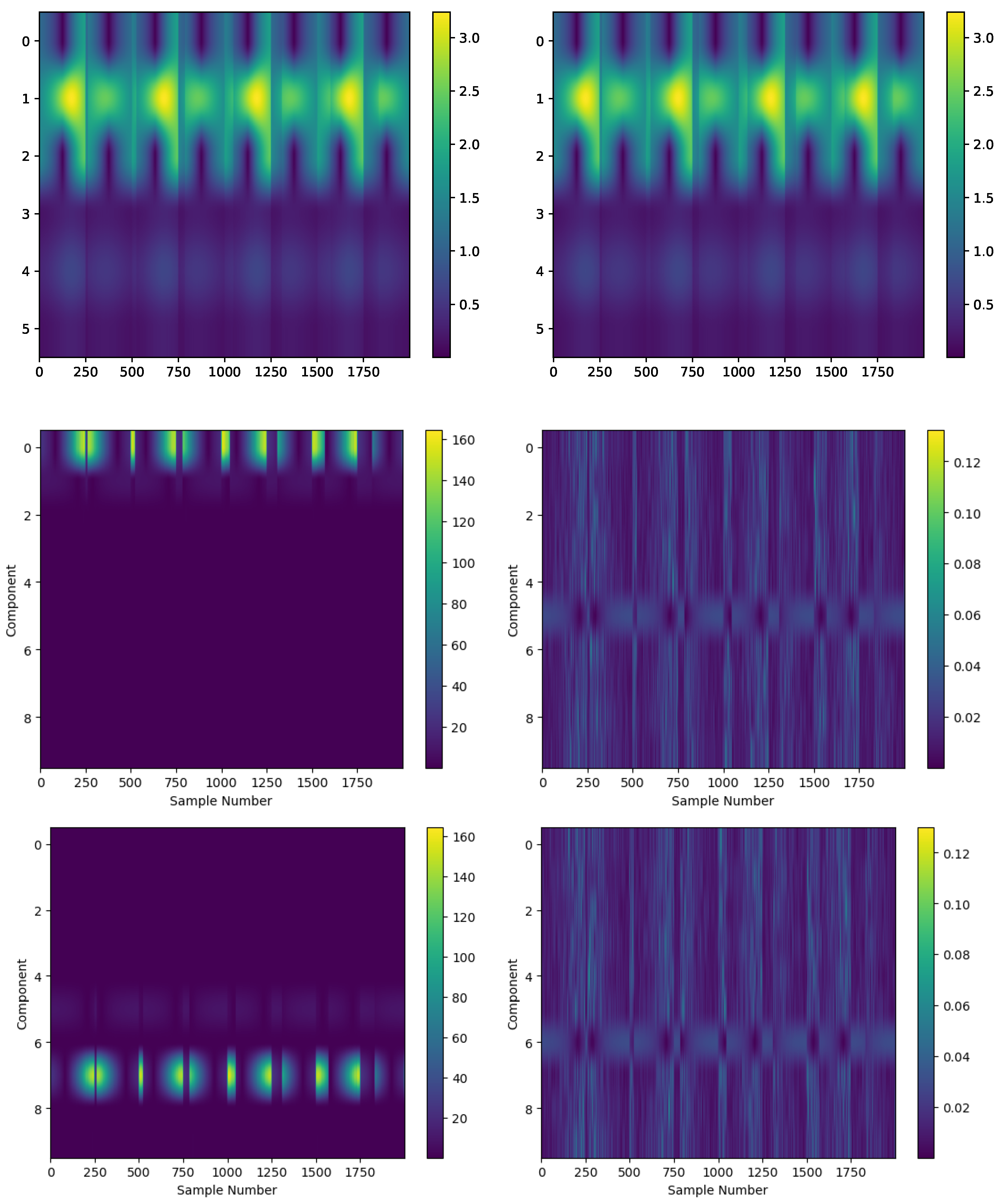
Comparison: LCON and LEXP

From Figure 17 and Figure 18, we can see the difference in extracted components using the two methods. Both cases extract peaks around the 200 sample mark, reflecting the signal’s concentrated information. LEXP show a clear difference between the three methods: while all three find the same peaks, the Eigenvalue decomposition is far more “smeared” than either PCA or ICA. In this case, ICA isolates the narrowest frequency band as shown in Figure 17.

When we apply LCON, we can see that the Eigenvalue decomposition and PCA generate the same results as expected. These methods generate specific ranked components. However, we can see that the clustered ICA result matches the Eigenvalue response.

By comparing LCON and LEXP, we can see that the two methods often do not converge on the same solution, even if we solve for a similar number of components using a source-based method such as FastICA. By comparing Figure 11, we can see a clear difference in the expanded scores of FastICA and PCA, with PCA consistently recovering the same components. At the same time, FastICA decomposes existing sources to generate more. This means the impact of additive noise increases as we increase the number of sources, meaning that, for more non-linear examples, large portions of the information can be lost. This is especially clear in comparing Figure 17 and Figure 18, which shows that the components recovered by LCON and LEXP do not solve for the same components when applied to sufficiently non-linear problems. This suggests that the two approaches are better suited to different styles of problem.

5. Results

This paper shows the results of applying the two optimal latent discovery approaches, LCON and LEXP, to various datasets utilising several user-selected metrics. Combined with the proposed Hankelisation functionality, this allows for a more in-depth analysis of time series data that would be impossible to analyse using traditional methods.

In the cases of the simple sinusoids, the mixed signals, and the ECG data, LEXP allowed us to generate organised latent spaces using the FastICA as our choice of LVM. In these cases, the latent results are more interpretable, allowing us to see clear signals in the cases of sinusoids, mixed signals, and ECG data. Especially with the ECG data, this can be used as a pre-processing step, allowing us to see clear differences between the two classes of sample type. If we examine the un-augmented data in Figure 12 as well as in Figure 13, we can see that the noise added by the FastICA decomposition makes it unclear which components represent important information about the data. In these cases, the unranked components seem to simply show random noise; however, when ranking is applied to the components, we can see clear differences emerge in the structure of the two datasets, with the normal data dominated by one single main component, whereas the abnormal data are dominated by two components explaining two-thirds of the total score.

We can see the limits of the linear ranking and clustering methods depending on the input data. Often, in high-dimensional, highly non-linear datasets, methods such as FastICA will generate split singular components; this means that two identical but opposite signals will be extracted. This can often be countered by taking the norm of the signal as the input. Additionally, the clustered form is hampered by the iterative nature of FastICA, which leads to noisier extracted components and reduced component magnitude and information as the number of components increases. Over-corrections often occur in attempting to correct the noise added by the FastICA, and information can be lost.

This paper shows that the software use case simplifies the ICA process, allowing the FastICA algorithm to be applied to traditional PCA problems. Combined with the Hankelisation functionality, this allows for more in-depth analysis of time series data, such as trend analysis.

The addition of ranking, as well as scaling, means that we can more easily apply ICA, or any other linear method, to problems, and the addition of Hankelisation allows us to analyse more wide-ranging data than are potentially solvable with one choice of linear dimensionality reduction method [46]. In this case, LCON is useful when dealing with highly multi-channel signals, whereas LEXP can be applied to a wider range of input types.

Finally, we briefly showcase the importance of supplementing optimal latent discovery with LEXP in improving the performance of the LS-PIE algorithm with source-based LVMs. Not only does this help improve the ease of application of the algorithm, but it also increases the performance of large datasets as it ensures that minimal components are calculated.

6. Discussion

The LS-PIE algorithm extends various dimensionality reduction methods, simplifying the generation of latent vectors and organising the latent space according to the user’s chosen metric. When combined with Hankelisation, this facilitates more in-depth analysis of time series data, such as trend analysis and other signal processing tasks. This paper demonstrates that optimal latent discovery in LS-PIE simplifies the application of LVMs, using ICA as an example, and enables the FastICA algorithm to be applied to problems typically addressed by PCA. With the addition of Hankelisation, the analysis of both traditional multi-channel data and single-channel time series data is enhanced.

The application of these methods to traditionally un-ordered latent models such as ICA allows us to sort and order the independent components generated. By compressing or ranking, and sorting the resulting ICs we allow for the resulting latent spaces to be more interpretable. This can be seen clearly in Figure 12 as well as in Figure 13: in these cases, the un-ranked components appear as random noise before the application of LS-PIE. This promotes more meaningful, and focused, data analysis by more clearly showing underlying generative principles, as well as statistical differences between datasets. The separation of meaningful latent signals from random noise allows us to clearly distinguish between the two, for example, deriving clear sinusoids from seemingly random noise in Figure 6. This allows for more carefully directed, in-depth analysis in future steps.

The two optimal latent discovery methods included within the module, LCON and LEXP, facilitate the application of reconstruction-centred LVMs, such as ICA, to problems traditionally analysed using interpretation-centred LVMs. These methods help organise latent spaces, resulting in clearer and more meaningful outcomes. Hankelisation broadens the scope of data analysis, making it possible to apply linear dimensionality reduction methods to a wider range of data. For iterative models such as FastICA, LEXP allows for computationally efficient dataset analysis, reducing the computational load in cases where computational cost increases with the number of components. Conversely, LCON identifies more naturally occurring components but can become time consuming with large datasets. However, linear methods struggle to provide informative insights with the more non-linear datasets. This framework has been applied to a wide range of data, including financial, medical, and in-depth vibrational data, as well as traditional signal separation methods. It offers a novel approach by applying ICA to problems typically tackled with PCA, allowing for analysis without relying on the variance of components for signal separation, and instead applying metrics better suited to the nature of the problem.

This approach shows its merits in application to linear methods. The LS-PIE framework is designed to improve the latent representations generated by LVMs; currently, the implementation focuses on linear methods. Further research is needed to extend this framework to non-linear methods such as auto-encoders and other neural networks. Extending this method to include non-linear methods would allow for more detailed analysis of complicated datasets, such as vibrational data. A future implementation to improve the latent representations generated by auto-encoders should be explored in future research.

As this framework exists as a post-processing/structural framework designed to incorporate existing dimensionality reduction techniques, it is less computationally efficient than using un-augmented techniques. This is due to the repeated latent component calculations involved in LCON, and with methods such as FastICA, a large number of components needs to be solved. However, the algorithm makes up for the reduced computational efficiency by the improved interpretability of the resulting components. The complexity of the application depends on the methods used to rank/compress/expand the resulting latent components, user-specified metrics and optimal latent discovery approaches to properly compare the computational efficiency. From Figure 13 and Figure 18, we can see that the clustering approach is often sensitive to signal noise. This is especially true when applying iterative methods such as FastICA to large, non-linear datasets. In these cases, the excessive splitting of components can severely reduce the per-signal information so that the combined signals reflect the noise. However, this is consistent with methods such as Eigenvalue decomposition as seen in Figure 18.

Additionally, the optimality of the solutions found by LCON and LEXP depend on the LVM applied. For closed-form LVMs such as PCA, in which all components are solved, we can easily condense very large latent spaces across reducing numbers of components without re-solving the latent variables. This allows us to optimally compress the data. However, with approaches such as FastICA where the resulting components are dependent on the number of components generated, the model needs to be re-applied at each step, increasing the computational cost. In cases like these, the LEXP method allows us to iteratively solve for smaller solution matrices until an optimal solution is recovered.

7. Conclusions

This paper illustrates the potential and effectiveness of the LS-PIE methodology, demonstrating its competence even in scenarios with high non-linearity. This capability allows reconstruction-focused methods like FastICA to deliver results comparable to those of interpretation-focused methods like PCA. The ranking and scoring features of this approach enable a broader range of LVMs to address various problems. This is evident when comparing the ICA results shown in Figure 6 to the original FastICA results presented at the beginning of the paper. Additionally, the methodology’s applicability to real-world data is demonstrated in the analysis of the ECG data and the SAFE data.

The efficacy of this methodology is clear when comparing the ICA results with the original FastICA results presented earlier. The method also proves effective on real-world data, with latent expansion (LEXP) optimal latent discovery producing interpretable results without fine-tuning, unlike traditional FastICA.

Analysing the SAFE curve shows that using a variance-driven ranking metric yields similar scores for the extracted components. However, the ranked ICA algorithm is more resilient to noise than traditional PCA.

Comparing the newly proposed clustering transformation to traditional FastICA reveals that the reconstruction errors are comparable, but the latent space of latent condensing (LCON) is more interpretable. One limitation is that certain LVMs, like ICA, cannot generate components beyond the smallest dimension of the input matrix, restricting the LCON algorithm’s power for smaller datasets. In such cases, LEXP is a better option.

This paper introduces two approaches that aid in creating more organised and interpretable latent spaces. LCON with BIRCH or DBSCAN identifies naturally occurring components within a dataset, simplifying data structure understanding. LEXP grows the components sequentially, reducing necessary steps and ensuring sufficient information retention. Both algorithms enhance the application of LVMs like the FastICA algorithm, promoting more focused and deliberate data analysis.

Examining Figure 6 shows that the LS-PIE application generates more similar results between the two approaches. This behaviour stems largely from the choice of clustering/ranking algorithm. Using the dot product to rank extracted components aligns the results closer to PCA. This behaviour also arises from using raw ICs as a similarity metric, prioritising intrinsic component shape similarity. Applying other metrics allows for different dataset analyses.

In all scenarios, the latent spaces extracted by the LS-PIE-augmented FastICA are more meaningful and understandable to human observers than the un-augmented latent spaces produced by FastICA or similar methods.

References

- Wilke, D.N.; Heyns, P.S.; Schmidt, S. The Role of Untangled Latent Spaces in Unsupervised Learning Applied to Condition-Based Maintenance. In Modelling and Simulation of Complex Systems for Sustainable Energy Efficiency; Hammami, A., Heyns, P.S., Schmidt, S., Chaari, F., Abbes, M.S., Haddar, M., Eds.; Springer: Cham, Switzerland, 2022; pp. 38–49. [Google Scholar]
- Stevens, J.; Wilke, D.N.; Setshedi, I. Latent Space Perspicacity and Interpretation Enhancement (LS-PIE) Framework. arXiv 2023, arXiv:2307.05620. [Google Scholar]
- Liu, Y.; Li, Q. Latent Space Cartography: Visual Analysis of Vector Space Embeddings. Comput. Graph. Forum 2019, 38, 67–78. [Google Scholar] [CrossRef]
- Hyvärinen, A.; Oja, E. Independent Component Analysis: Algorithms and Applications. Neural Netw. 2000, 13, 411–430. [Google Scholar] [CrossRef]
- Jollife, I.T.; Cadima, J. Principal component analysis: A review and recent developments. Philos. Trans. R. Soc. Math. Phys. Eng. Sci. 2016, 374, 20150202. [Google Scholar] [CrossRef] [PubMed]
- Tharwat, A. Independent component analysis: An introduction. Appl. Comput. Inform. 2018, 17, 222–249. [Google Scholar] [CrossRef]
- Jaadi, Z. Principal Component Analysis (PCA): A Step-by-Step Explanation. Available online: https://builtin.com/data-science/step-step-explanation-principal-component-analysis (accessed on 31 May 2024).
- Toiviainen, M.; Corona, F.; Paaso, J.; Teppola, P. Blind source separation in diffuse reflectance NIR spectroscopy using independent component analysis. J. Chemom. 2010, 24, 514–522. [Google Scholar] [CrossRef]
- Choi, S.; Riken, A.C.; Park, H.M.; Lee, S.Y. Blind Source Separation and Independent Component Analysis: A Review. Neural Inf. Process. Lett. Rev. 2005, 6, 1. [Google Scholar]
- Cao, X.R.; Liu, R.W. General Approach to Blind Source Separation. IEEE Trans. Signal Process. 1996, 44, 562–571. [Google Scholar]
- Lever, J.; Krzywinski, M.; Altman, N. Points of Significance: Principal component analysis. Nat. Methods 2017, 14, 641–642. [Google Scholar] [CrossRef]
- Hyvärinen, A. What Is Independent Component Analysis? Available online: https://www.cs.helsinki.fi/u/ahyvarin/whatisica.shtml (accessed on 31 May 2024).
- De Lathauwer, L.; De Moor, B.; Vandewalle, J. An introduction to independent component analysis. J. Chemom. 2000, 14, 123–149. [Google Scholar] [CrossRef]
- Wiklund, K. The Cocktail Party Problem: Solutions and Applications. Ph.D. Thesis, McMaster University, Hamilton, ON, Canada, 2009. [Google Scholar]
- Brys, G.; Hubert, M.; Rousseeuw, P.J. A robustification of independent component analysis. J. Chemom. 2005, 19, 364–375. [Google Scholar] [CrossRef]
- Westad, F. Independent component analysis and regression applied on sensory data. J. Chemom. 2005, 19, 171–179. [Google Scholar] [CrossRef]
- Bach, F.R.; Jordan, M.I. Finding Clusters in Independent Component Analysis. In Proceedings of the 4th International Symposium on Independent Component Analysis and Blind Signal Separation (ICA2003), Nara, Japan, 1–4 April 2003. [Google Scholar]
- Widom, H. Hankel Matrices. Trans. Am. Math. Soc. 1966, 121, 1–35. [Google Scholar] [CrossRef]
- Yao, F.; Coquery, J.; Lê Cao, K.A. Independent Principal Component Analysis for biologically meaningful dimension reduction of large biological data sets. BMC Bioinform. 2012, 13, 24. [Google Scholar] [CrossRef]
- Zhao, X.; Ye, B. Similarity of signal processing effect between Hankel matrix-based SVD and wavelet transform and its mechanism analysis. Mech. Syst. Signal Process. 2009, 23, 1062–1075. [Google Scholar] [CrossRef]
- Wang, L.; Yang, D.; Chen, Z.; Lesniewski, P.J.; Naidu, R. Application of neural networks with novel independent component analysis methodologies for the simultaneous determination of cadmium, copper, and lead using an ISE array. J. Chemom. 2014, 28, 491–498. [Google Scholar] [CrossRef]
- Golyandina, N. On the choice of parameters in Singular Spectrum Analysis and related subspace-based methods. arXiv 2010, arXiv:1005.4374. [Google Scholar] [CrossRef]
- Broomhead, D.; King, G.P. Extracting qualitative dynamics from experimental data. Phys. D Nonlinear Phenom. 1986, 20, 217–236. [Google Scholar] [CrossRef]
- Zhang, T.; Ramakrishnan, R.; Livny, M. BIRCH: An efficient data clustering method for very large databases. In Proceedings of the 1996 ACM SIGMOD International Conference on Management of Data, SIGMOD’96, New York, NY, USA, 4–6 June 1996; pp. 103–114. [Google Scholar] [CrossRef]
- Ester, M.; Kriegel, H.P.; Sander, J.; Xu, X. A Density-Based Algorithm for Discovering Clusters in Large Spatial Databases with Noise. In Proceedings of the 2nd International Conference on Knowledge Discovery and Data Mining (KDD), Portland, OR, USA, 2–4 August 1996; AAAI Press: Washington, DC, USA, 1996; pp. 226–231. [Google Scholar]
- Schubert, E.; Sander, J.; Ester, M.; Kriegel, H.P.; Xu, X. DBSCAN revisited, revisited: Why and how you should (still) use DBSCAN. ACM Trans. Database Syst. (TODS) 2017, 42, 19. [Google Scholar] [CrossRef]
- Ankerst, M.; Breunig, M.M.; Kriegel, H.P.; Sander, J. OPTICS: Ordering points to identify the clustering structure. ACM SIGMOD Rec. 1999, 28, 49–60. [Google Scholar] [CrossRef]
- Schubert, E.; Gertz, M. Improving the Cluster Structure Extracted from OPTICS Plots. In Proceedings of the Conference “Lernen, Wissen, Daten, Analysen” (LWDA), Mannheim, Germany, 22–24 August 2018; pp. 318–329. [Google Scholar]
- Comaniciu, D.; Meer, P. Mean shift: A robust approach toward feature space analysis. IEEE Trans. Pattern Anal. Mach. Intell. 2002, 24, 603–619. [Google Scholar] [CrossRef]
- Frey, B.J.; Dueck, D. Clustering by Passing Messages Between Data Points. Science 2007, 315, 972–976. [Google Scholar] [CrossRef] [PubMed]
- Dueck, D. Affinity Propagation: Clustering Data by Passing Messages. Ph.D. Thesis, University of Toronto, Toronto, ON, Canada, 2009. [Google Scholar]
- Kaoungku, N.; Suksut, K.; Chanklan, R.; Kerdprasop, K.; Kerdprasop, N. The silhouette width criterion for clustering and association mining to select image features. Int. J. Mach. Learn. Comput. 2018, 8, 69–73. [Google Scholar] [CrossRef]
- Yuan, C.; Yang, H. Research on K-Value Selection Method of K-Means Clustering Algorithm. J 2019, 2, 226–235. [Google Scholar] [CrossRef]
- Tibshirani, R.; Walther, G.; Hastie, T. Estimating the number of clusters in a data set via the gap statistic. J. R. Stat. Soc. Ser. B (Stat. Methodol.) 2001, 63, 411–423. [Google Scholar] [CrossRef]
- Davies, D.L.; Bouldin, D.W. A Cluster Separation Measure. IEEE Trans. Pattern Anal. Mach. Intell. 1979, PAMI-1, 224–227. [Google Scholar] [CrossRef]
- Caliński, T.; Harabasz, J. A dendrite method for cluster analysis. Commun. Stat. 1974, 3, 1–27. [Google Scholar] [CrossRef]
- Dokmanic, I.; Parhizkar, R.; Ranieri, J.; Vetterli, M. Euclidean Distance Matrices: Essential Theory, Algorithms and Applications. IEEE Signal Process. Mag. 2015, 32, 12–30. [Google Scholar] [CrossRef]
- Singh, A. K-means with Three different Distance Metrics. Int. J. Comput. Appl. 2013, 67, 13–17. [Google Scholar] [CrossRef]
- Lahitani, A.R.; Permanasari, A.E.; Setiawan, N.A. Cosine similarity to determine similarity measure: Study case in online essay assessment. In Proceedings of the 2016 4th International Conference on Cyber and IT Service Management, Bandung, Indonesia, 26–27 April 2016; pp. 1–6. [Google Scholar] [CrossRef]
- Ghorbani, H. Mahalanobis distance and its application for detecting multivariate outliers. Facta Univ. Ser. Math. Inform. 2019, 34, 583. [Google Scholar] [CrossRef]
- Davies, M.E.; James, C.J. Source separation using single channel ICA. Signal Process. 2007, 87, 1819–1832. [Google Scholar] [CrossRef]
- Kachuee, M.; Fazeli, S.; Sarrafzadeh, M. ECG Heartbeat Classification: A Deep Transferable Representation. In Proceedings of the 2018 IEEE International Conference on Healthcare Informatics (ICHI), New York, NY, USA, 4–7 June 2018. [Google Scholar] [CrossRef]
- Setshedi, I.I.; Loveday, P.W.; Long, C.S.; Wilke, D.N. Estimation of rail properties using semi-analytical finite element models and guided wave ultrasound measurements. Ultrasonics 2019, 96, 240–252. [Google Scholar] [CrossRef]
- Setshedi, I.I.; Wilke, D.N.; Loveday, P.W. Feature detection in guided wave ultrasound measurements using simulated spectrograms and generative machine learning. NDT E Int. 2024, 143, 103036. [Google Scholar] [CrossRef]
- Loveday, P.W.; Long, C.S.; Ramatlo, D.A. Ultrasonic guided wave monitoring of an operational rail track. Struct. Health Monit. 2020, 19, 1666–1684. [Google Scholar] [CrossRef]
- Djuwari, D.; Kumar, D.K.; Palaniswami, M. Limitations of ICA for Artefact Removal. Conf. Proc. IEEE Eng. Med. Biol. Soc. 2005, 2005, 4685–4688. [Google Scholar] [CrossRef] [PubMed]
Disclaimer/Publisher’s Note: The statements, opinions and data contained in all publications are solely those of the individual author(s) and contributor(s) and not of MDPI and/or the editor(s). MDPI and/or the editor(s) disclaim responsibility for any injury to people or property resulting from any ideas, methods, instructions or products referred to in the content. |
© 2024 by the authors. Licensee MDPI, Basel, Switzerland. This article is an open access article distributed under the terms and conditions of the Creative Commons Attribution (CC BY) license (https://creativecommons.org/licenses/by/4.0/).
Share and Cite
Stevens, J.; Wilke, D.N.; Setshedi, I.I. Enhancing LS-PIE’s Optimal Latent Dimensional Identification: Latent Expansion and Latent Condensation. Math. Comput. Appl. 2024, 29, 65. https://doi.org/10.3390/mca29040065
Stevens J, Wilke DN, Setshedi II. Enhancing LS-PIE’s Optimal Latent Dimensional Identification: Latent Expansion and Latent Condensation. Mathematical and Computational Applications. 2024; 29(4):65. https://doi.org/10.3390/mca29040065
Chicago/Turabian StyleStevens, Jesse, Daniel N. Wilke, and Isaac I. Setshedi. 2024. "Enhancing LS-PIE’s Optimal Latent Dimensional Identification: Latent Expansion and Latent Condensation" Mathematical and Computational Applications 29, no. 4: 65. https://doi.org/10.3390/mca29040065
APA StyleStevens, J., Wilke, D. N., & Setshedi, I. I. (2024). Enhancing LS-PIE’s Optimal Latent Dimensional Identification: Latent Expansion and Latent Condensation. Mathematical and Computational Applications, 29(4), 65. https://doi.org/10.3390/mca29040065