Article

A Corruption Impunity Model Considering Anticorruption Policies

by
Sandra E. Delgadillo-Alemán
1,*,
Roberto A. Kú-Carrillo
1 and
Alejandra Torres-Nájera
2
1
Departamento de Matemáticas y Física, Universidad Autónoma de Aguascalientes, Av. Universidad 940, Cd. Universitaria, Aguascalientes C.P. 20100, Mexico
2
Centro de Investigación en Matemáticas-Unidad Aguascalientes, Calzada de la Plenitud 103, Fracc. José Vasconcelos Calderón, Aguascalientes C.P. 20100, Mexico
*
Author to whom correspondence should be addressed.
Math. Comput. Appl. 2024, 29(5), 81; https://doi.org/10.3390/mca29050081
Submission received: 6 June 2024 / Revised: 2 September 2024 / Accepted: 9 September 2024 / Published: 14 September 2024

Abstract

:
Corruption is a global problem that affects the fair distribution of wealth of every country to different degrees and represents a problem to be solved to prevent the diversion and waste of resources. Among the different efforts to first measure it and later reduce it by proposing strategies, there exist a variety of indices, such as the corruption perception index, and other related issues, such as the global impunity index, the laxness of anticorruption policies, etc., which are computed for different countries worldwide. Based on these indices, we propose a model for corruption using a system of ordinary differential equations, considering anticorruption policies. Those three factors were identified after analyzing the phenomenon and available data, particularly for Mexico. Also, we fit it to the reported data of this country and perform simulations expecting to predict the short term, and performed a sensitivity analysis. The model is capable of reproducing the observed oscillatory behavior of the phenomenon. The model fit can still be improved by including the data for the anticorruption policies, which were only studied for different scenarios. Moreover, the model is susceptible to application in other countries, as long as data are available, and then provides a computational tool to predict and visualize the effect of appropriate public policies to fight corruption.

1. Introduction

Corruption is a major problem worldwide as numerous studies have shown that it occurs in the different spheres of society, causing a negative impact on the development of any country. For example, it causes damage to the economics of a country or the well-being of society simply because it implies a diversion of resources [1,2,3,4].
However, what exactly is corruption? We use the Transparency International definition: the abuse of power, public or private, for one’s benefit; see [5]. This definition implies that we may find it in public or private offices. However, the term corruption is often associated with government or political corruption, or activities whereby a public office is used to satisfy the personal interests of a public officer, against a country’s laws [6]. This is the type of corruption we aim to model mathematically.
When constructing a mathematical model, the first question that arises is how the variables are quantified. In this case, to measure corruption is a major challenge in political science and economics due to its inherently undercover nature. A comprehensive reference on this subject can be found in the work of Gnaldi et al. [7], where the techniques to measure the corruption are revised. There, it is mentioned that there are three types of indices/indicators to account for corruption: (i) perception-based indicators of corruption obtained through surveys of experts on different related subjects, (ii) ‘objective’ indicators of corruption based on company reports on the corruption cases they faced when starting a business in a country, and (iii) judiciary measures of corruption, which take into account judicial deeds, sentences, and corrupt crimes. Each of them has pros and cons. For example, perception-based indicators could be biased by a country’s media or economic growth. While the indicator based on company reports has its merits, it is important to exercise caution in its use, especially in cross-country studies where different judicial systems are in place. Judicial-related indicators could be of partial use for preventing corruption, as a conviction for corruption crimes may occur many years after the event took place, or an increased level of efficacy in the judicial system may reflect the efficacy of the system rather than an increased level of corruption. There are more advanced ways to measure corruption. Some of them are based on the assessment of anticorruption strategies. Others are based on the implementation of advanced computational techniques such as data mining and artificial intelligence, which are looking to automate the analysis of data generated, for example, by government websites.
As a modeling starting point, and with the aim of counting with data, we opted to use a classic index, Transparency International’s Corruption Perceptions Index (CPI), given the large amount of data over relatively long periods of time. It is based on opinions of experts and citizens to gauge the level of corruption within a country. It is important to remark that we could use a different corruption indicator/index in the modeling process, and it would not affect the process.
The Corruption Perception Index (CPI) reports yearly on the situation of 180 countries. This index ranks countries’ corruption based on opinion surveys and expert assessments. In this study, we assume that the CPI is an approximation for the actual corruption of a nation. This index ranges from 0 to 100 for the perceived level of corruption, where zero indicates a country with a high level of this problem, while 100 stands for a corruption-free government. Let us say that this index has been applied to encourage the development of measures and/or programs to combat the countries’ internal corruption. These studies provide useful information for a country to implement actions to avoid corruption, and mathematical models can help to make predictions under certain assumptions.
In our literature review on the mathematical modeling of corruption, we found some models from the economics point of view; see [8] for an overview. We may mention the classic work by Rose-Ackerman [9], which proposes a model to analyze the relationship between the clarity of the government requests and the market structure on corrupt dealings in the context of government purchases. It is concluded that the market structure and precise specifications of the products are important factors to reduce this type of misconduct. In [10], one can find a comprehensive, up-to-date and interdisciplinary discussion on the anticorruption policies of governments and anticorruption agencies across Europe.
Another mathematical modeling approach intends to model political and sociological behaviors related to corruption. For example, the evolutionary dynamical model described in [11] proposes mechanisms of evolutions of corruption by considering efficient government institutions, vote buying, and voting as a control mechanism of corruption in terms of a system of differential equations. Another related example is presented in [12] in terms of a mean-field game.There is also an abundant amount of the literature that considers corruption as an epidemiological disease [13,14]. In those models, populations are typically defined as susceptible to corruption, corrupt, recovered from corruption, and the like. Its analysis comprehends states of the free-of-corruption equilibrium and computes the analog to the basic reproductive number. Based on this number, we can say whether or not corruption can be eradicated in given circumstances. Moreover, several other works include optimal control strategies to reduce it, such as those in the study in [14,15,16]. Another approach is the application of agent-based models which, through computer simulations and defined rules that involve probability, emulate the dynamics of these systems; see, for example, [17] for a more recent and panoramic work. On the other hand, several studies aim to find the causes and consequences of corruption worldwide and to keep a record of its evolution to describe its behavior over time; see, for example, [18]. With this background, we wonder if it is possible to build a simple model in differential equations whose variables can be calculated from abundant data reported in the literature for several countries, which at a given time allows the calibration of the model and makes predictions on the increment/decrement of corruption, at least in the short term. We claim that the answer to this question is positive by considering important factors as model variables.
Another variable we will include in our model is impunity, which is defined, according to the UN, as “the impossibility, de jure or de facto, of bringing the perpetrators of violations to account-whether in criminal, civil, administrative or disciplinary proceedings-since they are not subject to any inquiry that might lead to their being accused, arrested, tried and, if found guilty, sentenced to appropriate penalties, and to making reparations to their victims” [19]. Again, measuring impunity is complicated, but it can be done indirectly via opinion polls that ask people about the wrongs suffered and the attention given to their case by the corresponding justice system. According to various sources, in the case of Mexico, there are high levels of impunity as presented in the survey in [20], which provides a clear view of the percentages of impunity. On the other hand, researchers from the University of the Americas Puebla (UDLAP) have proposed an index to measure the levels of impunity. It is called the Index of Global Impunity (IGI), and it has been computed since 2015 for various countries. In [21], the methodology to calculate the index is described. The construction of the index is carried out through three components: the structural and functional dimensions and human rights. The structural dimension refers to the state’s capacity to promote and impart justice. The functional dimension emphasizes measuring the actual performance of the institutions of the justice system. And finally, the human rights dimension focuses on the protection of the physical integrity of citizens. Then, we will consider the reported CPI and IGI data from 2015 to 2022 in our model.
The last variable that we consider is related to the policies against corruption. In the case of Mexico, various government offices take measures, such as the one described in [22], to combat this phenomenon. Among the anticorruption strategies, we may mention the supervision of the public budget, which is carried out by the Superior Audit Office of the Federation in Mexico. Also, programs of fiscal transparency can be implemented. They aim to provide general information on government actions in financial and fiscal sectors. Another strategy is the fiscal inspection to review and verify government office financial transactions. Although the purpose of auditing is not only to detect acts of corruption, it can help prevent them and stop them from leading to future economic deficiencies in institutions. In Mexico, the National Control System was created in 2010 in order to establish various strategies to promote the exchange of information to improve the control of public resources. Based on this information, we consider a variable to model how relaxed or strict the anticorruption policies are. For these variables, we did not find a specific index or data in the literature. Still, we will set possible scenarios according to the low, medium, and high values of this variable.
In this paper, our general objective is to propose a simple ordinary differential model, different from the epidemiological approach, in ordinary differential equations for the dynamics of corruption based on the main factors that affect this problem and which is capable of reconstructing the data available in the literature for a given country which lead to the prediction of the corruption forecast. To resolve this issue, we propose identifying factors related to corruption and propose a model in differential equations for an index of corruption that incorporates some of the factors above: the CPI, the IGI and the laxness of anticorruption policies. Next, we analyze the asymptotic behavior of its solutions to characterize it, adjust this model to the index data, and make simulations of possible scenarios with their corresponding interpretations.
The article is organized as follows. In Section 2, we define the variables and construct the corruption model based on two indices reported in the literature. Section 3.1 presents a classical analysis of the model equilibria and their asymptotic stability. In contrast, in Section 3.2, we calibrate the model using the reported data for the CPI and IGI for Mexico. Also, numerical simulations of the model solution are presented, assuming different scenarios according to the anticorruption policies, and compute a sensitivity analysis in Section 3.3. Finally, in Section 4, conclusions are presented.

2. Materials and Methods

In this section, we describe the variables and assumptions made to construct the differential equation model.

Mathematical Model for the CPI

Let us start by defining the variables for our model. The first one is the corruption variable, C ( t ) , defined in terms of the corruption perception index (CPI), and indicates the level of corruption at time t . As we previously mentioned, the CPI is an indirect measure of the corruption of a country and ranges from 0 to 100. To take advantage of the wealth of information available from this index, we define it as
C ( t ) = 100 C P I 100 .
Note that we are inverting the CPI scale and normalizing it, making it take values in the interval of [ 0 , 1 ] . When C ( t ) = 0 , it means zero corruption is occurring and corresponds to a CPI value equal to 100 . In an analog way, a value of the C ( t ) = 1 is consistent with a CPI value equal to 0, implying a country with an extremely high value of corruption.
The second variable is the proportion of corrupt acts sued for and punished by the law, L ( t ) , which is the level of pusnished/sued corruption cases at time t . The definition of this variable may be odd, as we are assuming that this variable is the opposite of impunity. Then, we can use the Impunity Global Index, the IGI, to define this variable as the complement and normalization of the IGI,
L ( t ) = 100 I G I 100 .
Note that 0 stands for zero punished or sued cases (total impunity), and 1 means that all the corrupt cases are punished or sued (zero impunity), corresponding to an IGI of 0 and 100 , respectively.
The third variable is the laxness of the anticorruption policies, P ( t ) , which is the level of laxness of anticorruption policies at time t . A small value of this variable means strict anticorruption policies, and conversely, a high one implies relaxed or null anticorruption policies. The role of this variable is to model the regulation and/or transparency processes in the government. In this case, we did not find the reported measurements matching our definition, so we will analyze the model for different synthetic levels:we assigned values of the coefficients of Equation (5) to be able to compute the simulations.
Let us elaborate on assumptions made in the modeling process. In the first equation of our model, we assume that the corruption grows in proportion to the product of the corruption, C ( t ) , and the ease/laxness of anticorruption policies, P ( t ) . On the other side, it decreases proportionally to the interaction of the corruption, C ( t ) , and the acts punished/sued for, L ( t ) ,
C ˙ ( t ) = α C ( t ) P ( t ) γ 1 C ( t ) L ( t ) ,
where α and γ 1 are positive parameters. Then, corruption grows as long as there is corruption and the anticorruption policies are lax, while it is discouraged as more corruption cases are punished/sued.
In the second equation, we assume that the growth rate of punished corruption cases is in proportion to the interaction of the corruption, C ( t ) , and the punished cases, L ( t ) , while it decreases in proportion to the punished/sued cases, L ( t ) ,
L ˙ ( t ) = β L ( t ) + γ 2 C ( t ) L ( t ) .
Note that this variable will increase if we have a high number of corruption and punished cases, and if C ( t ) = 0 , then L ( t ) goes to zero, as time goes over, meaning that in the absence of corruption, there will not cases to prosecute. The positive parameters β and γ 2 are the rates decrease and the growth of sued or sanctioned cases, respectively.
The third equation of the model stands for the growth rate of the laxness of anticorruption policies, P ( t ) . It was essentially proposed as a logistic equation, diminished by a linear term proportional to corruption, C ( t ) ,
P ˙ ( t ) = δ P ( ξ P ( t ) ) ϵ C ( t ) .
Its logistic nature indicates to us that in the long term, its solution will tend to an equilibrium solution, ξ , which we consider, the projected level or goal value of the laxness of anticorruption policies; meanwhile, the natural growth rate is δ ξ . The term ϵ C ( t ) plays the role of the sensitivity or promptness to the level of corruption in implementing anticorruption policies, whereas ϵ is the sensitivity of policy change to the perceived corruption of the authorities. A high value of ϵ will cause a decrement in the growth rate of the laxness of anticorruption policies, and conversely, a low value does not reduce P ( t ) , making it grow or remain at a certain level. The selection of the modeling terms in this system of equations was inspired by the Lotka–Volterra system of equations, which tries to capture the oscillatory behavior of variables C ( t ) and L ( t ) while the logistic equations for variable P ( t ) were elected to emulate a changing variable from the level to the carrying capacity.
In the next section, we analyze the asymptotic behavior of the model, Equations (3)–(5), when C ( t ) , L ( t ) , P ( t ) 0 and all the model’s coefficients are positive constants.

3. Results

In this section, we carry out the classic asymptotic analysis of the system of differential equation model and determine the conditions for the stability of its equilibrium solutions.

3.1. Analysis of the Model

Let us start by computing the equilibrium points of the system of differential equations by solving the homogeneous system ( C ˙ , L ˙ , P ˙ ) = ( 0 , 0 , 0 ) ,
α C P γ 1 C L = 0 , β L + γ 2 C L = 0 , δ P ( ξ P ) ϵ C = 0 .
We denote each equilibrium point i by E i = ( C i , L i , P i ) , i N . It turns out that we obtain four equilibrium points: E 1 = ( 0 , 0 , 0 ) , E 2 = ( 0 , 0 , ξ ) , E 3 = β γ 2 , α γ 1 P 1 , P 1 and E 4 = β γ 2 , α γ 1 P 2 , P 2 where
P 1 , 2 = ξ δ ± ( ξ δ ) 2 4 δ ϵ β γ 2 2 δ ,
and we have assumed that ( ξ δ ) 2 4 δ ϵ β γ 2 > 0 . Note that in case ( ξ δ ) 2 4 δ ϵ β γ 2 = 0 , we obtain only three equilibrium points because E 3 = E 4 . Now, in order to analyze the stability of those points, we calculate the Jacobian matrix,
J = α P γ 1 L γ 1 C α C γ 2 L γ 2 C β 0 ϵ 0 δ ξ 2 δ P
which we will evaluate at each equilibrium point.
For E 1 = ( 0 , 0 , 0 ) , this matrix becomes
J | ( 0 , 0 , 0 ) = 0 0 0 0 β 0 ϵ 0 δ ξ
whose eigenvalues are λ 1 = 0 , λ 2 = β < 0 and λ 3 = δ ξ > 0 . Then, E 1 is unstable, implying that this state cannot be reached. From the modeling point of view, E 1 represents a state where there are no corruption nor punished/sued corruption cases, and the anticorruption policies are highly restrictive, which could cause problems in spending the public budget.
For E 2 = ( 0 , 0 , ξ ) , the Jacobian matrix evaluated at the equilibrium point is
J | ( 0 , 0 , ξ ) = α ξ 0 0 0 β 0 ϵ 0 δ ξ .
In this case, its eigenvalues are λ 1 = α ξ > 0 , λ 2 = β < 0 and λ 3 = δ ξ < 0 . Then, E 2 also is unstable. This point is interpreted as the case where the corruption is 0, meaning that the country is very clear of corruption. There are no cases of punished corruption, and the policies for the budget exercise have reached a limit, which is in terms of the projected level of anticorruption policies, ξ , and the sensibility to the corruption acts, ϵ . However, this equilibrium state cannot be reached because the equilibrium point E 2 is unstable.
For equilibrium E 3 = ( β γ 2 , α γ 1 P 1 , P 1 ) , where P 1 = ξ δ + ( ξ δ ) 2 4 δ ϵ β γ 2 2 δ , the Jacobian matrix evaluated at this point is given by:
J 3 = J | ( β γ 2 , α γ 1 P 1 , P 1 ) = α P 1 γ 1 α γ 1 P 1 γ 1 β γ 2 α β γ 2 γ 2 α γ 1 P 1 γ 2 β γ 2 β 0 ϵ 0 δ ξ 2 δ P 1 , ,
= 0 β γ 1 γ 2 α β γ 2 α γ 2 γ 1 P 1 0 0 ϵ 0 δ ξ 2 δ P 1 .
Then, its corresponding characteristic polynomial is given by:
p ( λ ) = det ( J 3 λ I ) = λ β γ 1 γ 2 α β γ 2 α γ 2 γ 1 P 1 λ 0 ϵ 0 δ ξ 2 δ P 1 λ ,
p ( λ ) = λ 3 + δ ( ξ 2 P 1 ) λ 2 α β ( P 1 + ϵ γ 2 ) λ + α β δ ( ξ 2 P 1 ) P 1 .
To determine the eigenvalues, we must solve the equation p ( λ ) = 0 , or equivalently,
λ 3 δ ( ξ 2 P 1 ) λ 2 + α β ( P 1 + ϵ γ 2 ) λ α β δ ( ξ 2 P 1 ) P 1 = 0 ,
which is more complex. However, in this case, we will use Routh–Hurwitz’s criterion [23] to determine the conditions for the eigenvalues to have a negative real part, which are the following:
a 0 = 1 > 0 , a 1 = δ ( ξ 2 P 1 ) > 0 , a 2 = α β δ ( P 1 + ϵ γ 2 ) > 0 ,
a 3 = δ α β ( ξ 2 P 1 ) P 1 > 0 , b 1 = a 2 a 1 a 3 a 0 a 2 > 0 ,
which are satisfied as long as ξ < 2 P 1 and P 1 > 0 . Note that P 1 > 0 and also ξ < ξ + ( ξ δ ) 2 4 δ ϵ β γ 2 δ = 2 P 1 . Therefore, E 3 = ( β γ 2 , α γ 1 P 1 , P 1 ) is an asymptotically stable equilibrium point. Having this nature, the close solutions to this point tend to it, i.e., the corruption level will tend to β γ 2 , and the anticorruption policies to P 1 , and the cases punished/sued to α γ 1 P 1 .
For E 4 = ( β γ 2 , α γ 1 P 2 , P 2 ) , note that the Jacobian matrix evaluated at this point has the same form as that for E 3 , but changing P 1 by P 2 . Then, the characteristic polynomial is
p ( λ ) = λ 3 + δ ( ξ 2 P 2 ) λ 2 α β ( P 2 + ϵ γ 2 ) λ + α β δ ( ξ 2 P 2 ) P 2 .
Analogously, the Routh–Hurwitz criterion is applied to determine the conditions for the eigenvalues to have a negative real part; these are again ξ < 2 P 2 and P 2 > 0 . However, since 2 P 2 = ξ δ ( ξ δ ) 2 4 δ ϵ β γ 2 δ = ξ ( ξ δ ) 2 4 δ ϵ β γ 2 δ ξ , then E 3 is unstable.
Remark 1.
If ( ξ δ ) 2 4 δ ϵ β γ 2 = 0 , we only have three equilibrium points of the system and this third one, ( β γ 2 , α ξ 2 γ 1 , ξ 2 ) has associated the characteristic polynomial
P ( λ ) = λ 3 α β ( ξ 2 + ϵ γ 2 ) λ .
Its corresponding eigenvalues are λ 1 = 0 , λ 2 , 3 = ± i α β ( ξ 2 + ϵ γ 2 ) , and therefore stability cannot be determined by this criterion. However, numerical experiments suggest unstable equilibrium points, E 3 and E 4 .

3.2. Data Fitting

In this section, we fit the model to data reported for the CPI and IGI in terms of the variables, previously defined. Let us say that not all the parameters were adjusted due to the lack of data. However, we propose values for those parameters to configure different scenarios. Next, we present simulations varying the levels of anticorruption policies. To finally, we discuss the simuations of the possible scenarios.
After a review of the literature, we find the time series available for the CPI and the IGI. In Table 1, we show the CPI obtained from the Transparency International website [24] from 2012 to 2021. Table 2 corresponds to the IGI data from 2015 to 2020, except for 2019 and 2021, which were not reported. Both Tables are of data for Mexico. Note that the number of data available is reduced, particularly for the global index of impunity. For this reason, a linear interpolation was carried out to have an approximate value for the years of 2019 and 2021.
In Figure 1, we can see graphically the evolution of both the data, in terms of the re-scaled variables, C ( t ) and L ( t ) , which correspond to the Corruption Perception and the Global Impunity Indices. Observe a slight oscillation for both C ( t ) and L ( t ) , but for the IGI variable, there is a more accentuated change in its growth trend in 2018. The above-mentioned trend indicates that the IPC variable, C ( t ) , has remained relatively the same in recent years, while the one that corresponds to the impunity index, L ( t ) , has decreased slightly from 2016 to 2018, where it began to grow more rapidly in 2018, and later in 2020, it decreased again; see Figure 1. Let us recall, that the COVID-19 pandemic hit the world in 2020, which may have has caused a modification in the data trend for the years of 2021 and 2022.
Our next step will be to adjust the model to the reported data.

3.3. Numerical Simulations

In this subsection, we describe the procedure performed for parameter fitting, as previously announced. First, we consider the data in Table 1 and Table 2 for the years of 2015 to 2020, where we linearly interpolate the IGI values for years 2019 and 2021 to fulfill the missing information. We also interpolate for the intermediate values of each interval, i.e., at the half of each year for each C i and L i . It is worth mentioning that linear interpolation assumes that the missing data is located on a straight line between the two known points. This is reasonable since the period between the two known data, 2018 to 2020 and 2020 to 2021, is two years each. We use them to calculate the missing annual values, those for 2019 and 2021, in the original time series. On the other hand, the interannual interpolation we performed was carried out to have more points to fit the model and, thus, have a curve closer to the fact that these data do not change quickly and to alleviate the small amount of data we have. With those values, we will carry out the parameter-fitting process.
We define the quadratic error function whose arguments are the parameters we seek to adjust as
E ( p ) = i = 1 n ( C i , L i , P i ) ( C i , L i , P i ) ,
where p is the vector of the parameters to fit, n denotes the number of data in the time series, ( C i , L i , P i ) is the vector of data at time t i and ( C i , L i , P i ) are the values generated by the model at times t i , for i = 1 , , n . To minimize this function, we employ the Nelder–Mead method, which has been widely applied in nonlinear optimization, and in our case, it converges quickly. As already mentioned, not all parameters were adjusted. In particular, we search for parameter vector p = ( α , β , γ 1 , γ 2 ) , and we proposed values for δ , ξ and ϵ , which are the parameters of Equation (5).
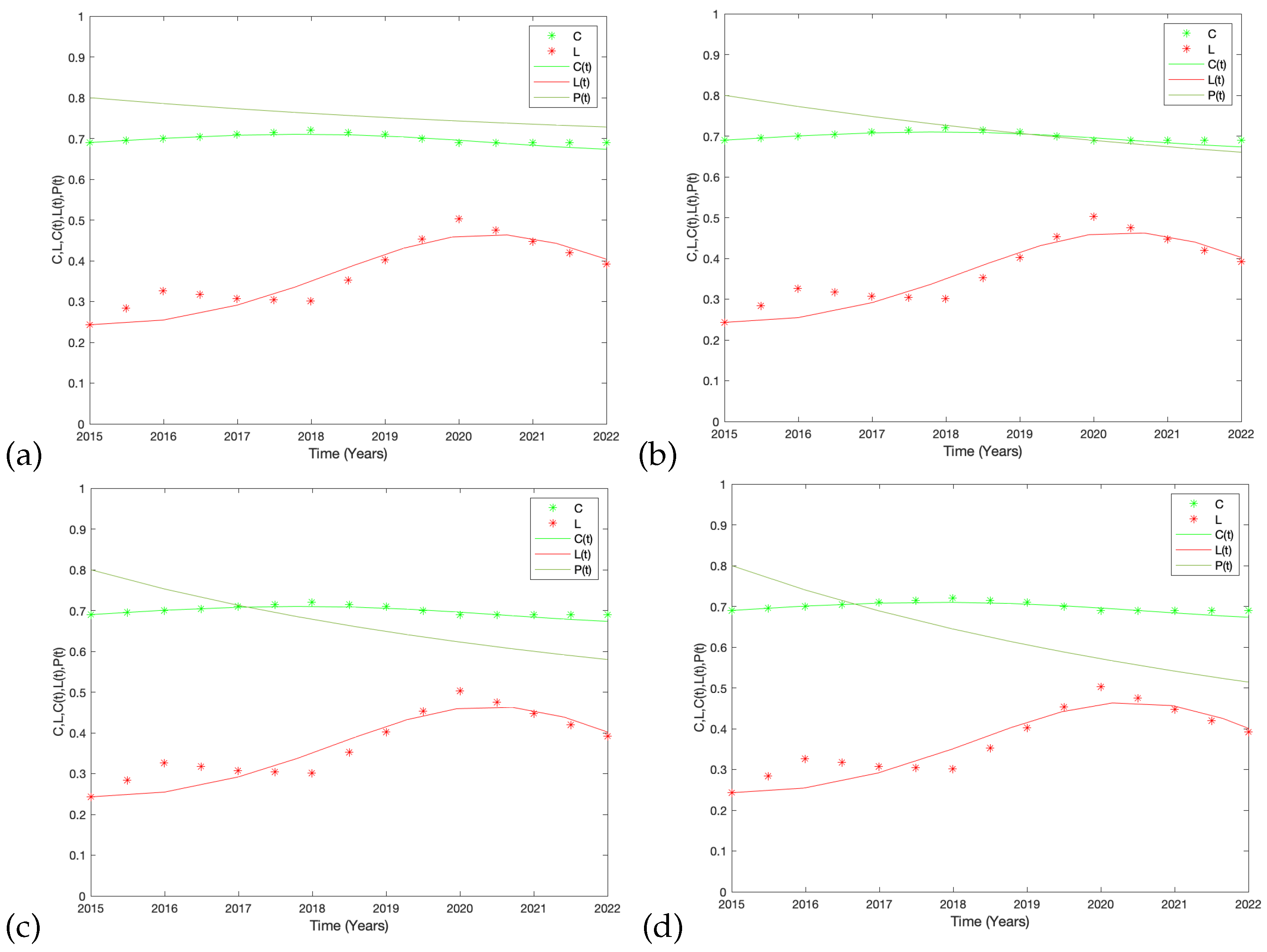
For the computational implementation, we use the built-in functions in Matlab, the fminsearch function and the routine ode23, corresponding to the Nelder–Mead method and the solver of the differential equation system, respectively. The minimum search was inicialiated with random parameter values in the interval of [ 0 , 1 ] , 5000 times for each case. Table 3 shows the results obtained with this procedure for different sets of fixed parameters δ , ξ and ϵ , that we vary to represent different scenarios regarding the flexibility of the anticorruption policies ( ξ ) and the sensitivity of the authorities towards the increase in corruption ( ϵ ). We thus have the following four cases: (a) flexible projected anticorruption policies with low sensitivity to corruption, (b) flexible projected anticorruption policies with high sensitivity, (c) strict projected anticorruption policies with low sensitivity and (d) strict projected anticorruption policies with high sensitivity. We have set δ = 0.15 for all these cases, while for the flexible and strict projected levels of anticorruption policies, we chose ξ = 0.7 and ξ = 0.4 , respectively. For the sensitivity of implementing anticorruption policies concerning corruption, the two scenarios we study are low and high sensitivity, ϵ = 0.005 and ϵ = 0.025 , respectively. Note that all these cases correspond to the existence of only two equilibrum points, E 1 and E 2 , as was described previously.
In Figure 2, we present graphically the simulations using the parameter values obtained in the fitting process for the four scenarios, presented in Table 3. The initial condition we have used is ( C ( 0 ) , L ( 0 ) , P ( 0 ) ) = ( 0.69 , 0.243 , 0.8 ) , i.e., we are considering that the corruption, C ( 0 ) = 0.69 , is equivalent to a C P I of 31, an L ( 0 ) = 0.243 equivalent to an I G I of 75.7 points, and that both values correspond to Mexico in the year of 2022. For variable anticorruption policy flexibility, we have used P ( 0 ) = 0.8 , meaning that the anticorruption policies are relaxed. Observe that we request the model to fit the data by assuming it corresponds to one of the given cases. For all cases, the model variable C ( t ) fits well for almost all data, which behaves with subtle oscillations. The model variable L ( t ) misses the first oscillation but captures the second one of the two that the data presents. Also, it captures the primary growth of this variable for the reported data. For variable P ( t ) , the laxness of the anticorruption policies decreases at a different rate depending on the level of the long term goal of anticorruption policies and the sensitivity to corruption. We have cases (a), (b), (c), and (d) in which the decreasing rate becomes more deep. The highest decreasing rate occurs at the strict projected level of anticorruption policies and high sensibility policies for corruption. Another characteristic of the model solutions is that the time the model predicts the maximum is reached after the data reports it occurred.
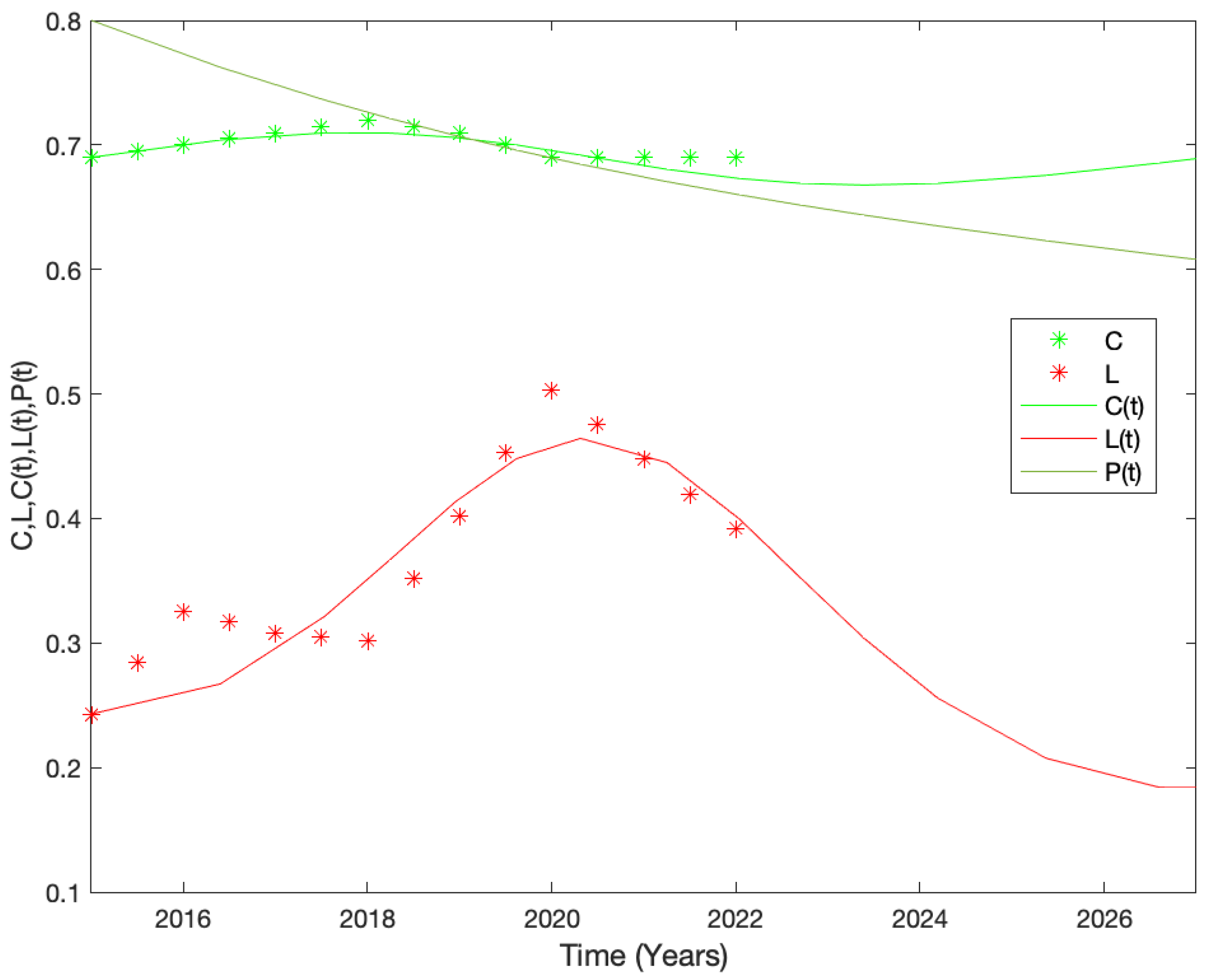
In Figure 3, we present case (b), which best approximates the data series according to the fitting error given in Table 3. Note that the error values are very similar between the different scenarios. This indicates that the model with the data used for the fitting cannot sharply discriminate between one scenario or another, suggesting that we are close to a point where the policies are changing from one scenario to another. If we look forward to a sharp discrimination in the cases, it is necessary to have a more extended time series to improve the adjustments. In addition, it would be necessary to know more about the behavior and effect of anticorruption policies over time, P ( t ) . The measurement of this variable presents a challenge and is an issue that must be included in future versions of this model. However, let us claim that model fitting succeeded. Then, this case corresponds to the flexible projected level of anticorruption policies and a high sensitivity to increase the laxness of these policies as corruption occurs. Let us remark that the Mexican government claims that corruption has been reduced, but this is not perceived by the population, as the CPI has remained at the same value for three years in a row. In this sense, our model fits the reality as, on the one hand, the sensibility of the authorities to fight corruption has increased, but this has not changed the perception of the corruption index.
From Figure 3, it can be seen that we have run the model for five more years, up to the year of 2027. As can be seen, the model has oscillatory behavior in the corruption and pusnished cases. However, for the corruption, its oscillation is low and keeps its value at almost the same level for 13 years. It is important to say that anticorruption policies become more strict as time passes, but this is not leading to a meaningful decrement in the corruption level which is a consequence of having a decrease in the number of punished corruption cases. According to the model, it is not enough to make projected level of anticorruption policies more strict, without a substancial growth of punished cases. Recall that this is equivalent to a decrement in the impunity. Also, other long term runs of the model show us that it is very sensitive to variable ϵ , which implies that we need to search other modelling strategies or for more information on the mechanisms and variables that inhibit corruption to incorporate them into the model.

3.4. Sensitivity Analysis

In this section, we performed a parameters sensitivity analysis for the model (3)–(5) to identify how the solutions depend on the variation of the system’s parameters. Our approach utilizes local sensitivity analysis with the help of Matlab, requesting the partial derivatives of the solutions with respect to the parameters when solving them numerically. In Figure 4, we have plotted the results for ten years, which show us that the second equation, for L ( t ) , is highly sensitive to parameters α , γ 1 , and ϵ . Note that in the previous section, we have already identified the great variability of the solutions when changing parameter ϵ , but we missed the high dependency on parameter α , which stands for the contribution of the interactions of the corruption and the laxness of the anticorruption policies, while parameter γ 1 accounts for the interaction between the corruption and the punished corruption cases (the complement of impunity). Then, it is important to find strategies inside these parameters to obtain more significant changes in the solutions of the model. This also tells us what parameters must be identified more carefully to contain the error propagation on the solutions. Note from Figure 4 that the variation of the solution with respect to the remaining parameters is not important as time goes on; moreover, the most affected equation is Equation (2), followed by Equation (3).

4. Conclusions

In this work, we have proposed a simple ordinary differential equation model for corruption based on essential factors such as impunity and anticorruption policies. It is important to emphasize that for the corruption and impunity variables, we have started from the data reported on the Perception of Corruption and the Global Impunity Index, for which there is data from many countries, although only for a few years. We want to highlight the importance of proposing a model based on the data reported in the literature. Furthermore, it considers the impunity variable to be strongly associated with corruption but absent in most ordinary diffential equation corruption models. Also, the strict policies are considered to be a variable in the model for which it was not possible to find a time series. For this variable, different scenarios were proposed that would allow us to show simulations to verify the progress of our approach numerically. Then, it was possible to adjust our model to the reported data and perform simulations to predict the behavior for subsequent years for the case of Mexico, which has a more extensive time series for the case of the IGI. With the identified parameters and varying the parameters related to anticorruption policies, we propose different scenarios and present simulations. Also, we were able to identify the sensibility of the equations to the parameters. It is important to mention the limitations of our model due to the lack of data, especially for the IGI, where few measurements were found. The fit can still be improved by refining and improving our model to provide the most accurate and useful predictions. However, we believe this model can be used as a calculation tool, enabling forecasts for any country. Let us remark that the proposed model can be used with other corruption and impunity indices, because the general assumption remains valid. With data from the CPI and the IGI, our model can offer the potential to predict and visualize effective public policies to combat corruption, which could significantly impact the global fight against corruption. Finally, in future work, we would like to propose a model that reproduces the oscillatory behavior more precisely by incorporating other variables and data.

Author Contributions

Conceptualization, S.E.D.-A. and R.A.K.-C.; investigation, S.E.D.-A., R.A.K.-C. and A.T.-N.; methodology, S.E.D.-A. and R.A.K.-C.; software, S.E.D.-A. and A.T.-N.; supervision, S.E.D.-A. and R.A.K.-C.; validation, S.E.D.-A.; writing—original draft, S.E.D.-A. and R.A.K.-C.; writing—review and editing, S.E.D.-A. and R.A.K.-C. All authors have read and agreed to the published version of the manuscript.

Funding

This research was funded by the Universidad Autónoma de Aguascalientes, grant numbers PIM-24-5 and PIM-24-6.

Data Availability Statement

All databases were taken from the cited literature.

Conflicts of Interest

The authors declare no conflicts of interest.

References

  1. d’Agostino, G.; Dunne, J.; Pieroni, L. Corruption and growth in Africa. Eur. J. Political Econ. 2016, 43, 71–88. [Google Scholar] [CrossRef]
  2. Serritzlew, S.; Sønderskov, K.M.; Svendsen, G.T. Do corruption and social trust affect economic growth? A review. J. Comp. Policy Anal. Res. Pract. 2014, 16, 121–139. [Google Scholar] [CrossRef]
  3. Gründler, K.; Potrafke, N. Corruption and economic growth: New empirical evidence. Eur. J. Political Econ. 2019, 60, 101810. [Google Scholar] [CrossRef]
  4. Ellis, C.J.; Fender, J. Corruption and transparency in a growth model. Int. Tax Public Financ. 2006, 13, 115–149. [Google Scholar] [CrossRef]
  5. Transparency-International. What Is Corruption? 2022. Available online: https://www.transparency.org/en/what-is-corruption (accessed on 5 June 2024).
  6. Khan, A.; Krishnan, S. Conceptualizing the impact of corruption in national institutions and national stakeholder service systems on e-government maturity. Int. J. Inf. Manag. 2019, 46, 23–36. [Google Scholar] [CrossRef]
  7. Gnaldi, M.; Del Sarto, S.; Falcone, M.; Troìa, M. Measuring corruption. In Understanding and Fighting Corruption in Europe: From Repression to Prevention; Springer Nature: Cham, Switzerland, 2021; pp. 43–71. [Google Scholar]
  8. Patra, A.; Matipira, L.; Saruchera, F.; Musti, K.S. Revisiting corruption mathematical models in the fourth industrial revolution. In Advanced Perspectives on Global Industry Transitions and Business Opportunities; IGI Global: Hershey, PA, USA, 2021; pp. 270–296. [Google Scholar]
  9. Rose-Ackerman, S. Corruption: A Study in Political Economy; Academic Press: Cambridge, MA, USA, 2013. [Google Scholar]
  10. Carloni, E.; Gnaldi, M. Understanding and Fighting Corruption in Europe: From Repression to Prevention; Springer Nature: Cham, Switzerland, 2021. [Google Scholar]
  11. Accinelli, E.; Martins, F.; Pinto, A.A.; Afsar, A.; Oliveira, B.M. The power of voting and corruption cycles. J. Math. Sociol. 2022, 46, 56–79. [Google Scholar] [CrossRef]
  12. Kolokoltsov, V.N.; Malafeyev, O.A. Mean-field-game model of corruption. Dyn. Games Appl. 2017, 7, 34–47. [Google Scholar] [CrossRef]
  13. Lemecha, L. Modelling corruption dynamics and its analysis. Ethiop. J. Sci. Sustain. Dev. 2018, 5, 13–27. [Google Scholar]
  14. Alemneh, H.T. Mathematical modeling, analysis, and optimal control of corruption dynamics. J. Appl. Math. 2020, 2020, 5109841. [Google Scholar] [CrossRef]
  15. Fantaye, A.K.; Birhanu, Z.K. Mathematical Model and Analysis of Corruption Dynamics with Optimal Control. J. Appl. Math. 2022, 2022, 8073877. [Google Scholar] [CrossRef]
  16. Yusuf, I.; Abdulrahman, S.; Musa, B.; Adamu, G. Controlling the spread of corruption through social media; a mathematical modelling approach. IOSR J. Math. 2016, 12, 75–81. [Google Scholar]
  17. Elnawawy M., S.; Okasha, A.E.; Hosny, H.A. Agent-based models of administrative corruption: An overview. Int. J. Model. Simul. 2022, 42, 350–358. [Google Scholar] [CrossRef]
  18. De la Poza, E.; Jódar, L.; Merello, P. Modeling Political Corruption in Spain. Mathematics 2021, 9, 952. [Google Scholar] [CrossRef]
  19. Orentlicher, D. Report of Commission on Human Rights of United Nations, 2005; United Nations: Geneva, Switzerland, 2005; Available online: https://www.ohchr.org/sites/default/files/Documents/AboutUs/annualreport2005.pdf (accessed on 5 June 2024).
  20. contra la corrupción y la impunidad, M. Tercera Encuesta Sobre la Corrupción y la Impunidad; REFORMA: Mexico city, Mexico, 2021; Available online: https://contralacorrupcion.mx/tercera-encuesta-nacional-sobre-corrupcion-e-impunidad/ (accessed on 5 June 2024).
  21. Le Clercq, J.A.; Rodríguez Sánchez Lara, G.R. Global Impunity Index 2020 (GII 2020). Impunity Levels in the World (April 30, 2021). Available online: https://ssrn.com/abstract=3837642 (accessed on 5 June 2024).
  22. Yap, J.B.H.; Lee, K.Y.; Rose, T.; Skitmore, M. Corruption in the Malaysian construction industry: Investigating effects, causes, and preventive measures. Int. J. Constr. Manag. 2022, 22, 1525–1536. [Google Scholar] [CrossRef]
  23. DeJesus, E.X.; Kaufman, C. Routh-Hurwitz criterion in the examination of eigenvalues of a system of nonlinear ordinary differential equations. Phys. Rev. A 1987, 35, 5288. [Google Scholar] [CrossRef] [PubMed]
  24. Transparency-International. 2021 Corruption Perceptions Index. 2022. Available online: https://www.transparency.org/en/cpi/2022 (accessed on 5 June 2024).
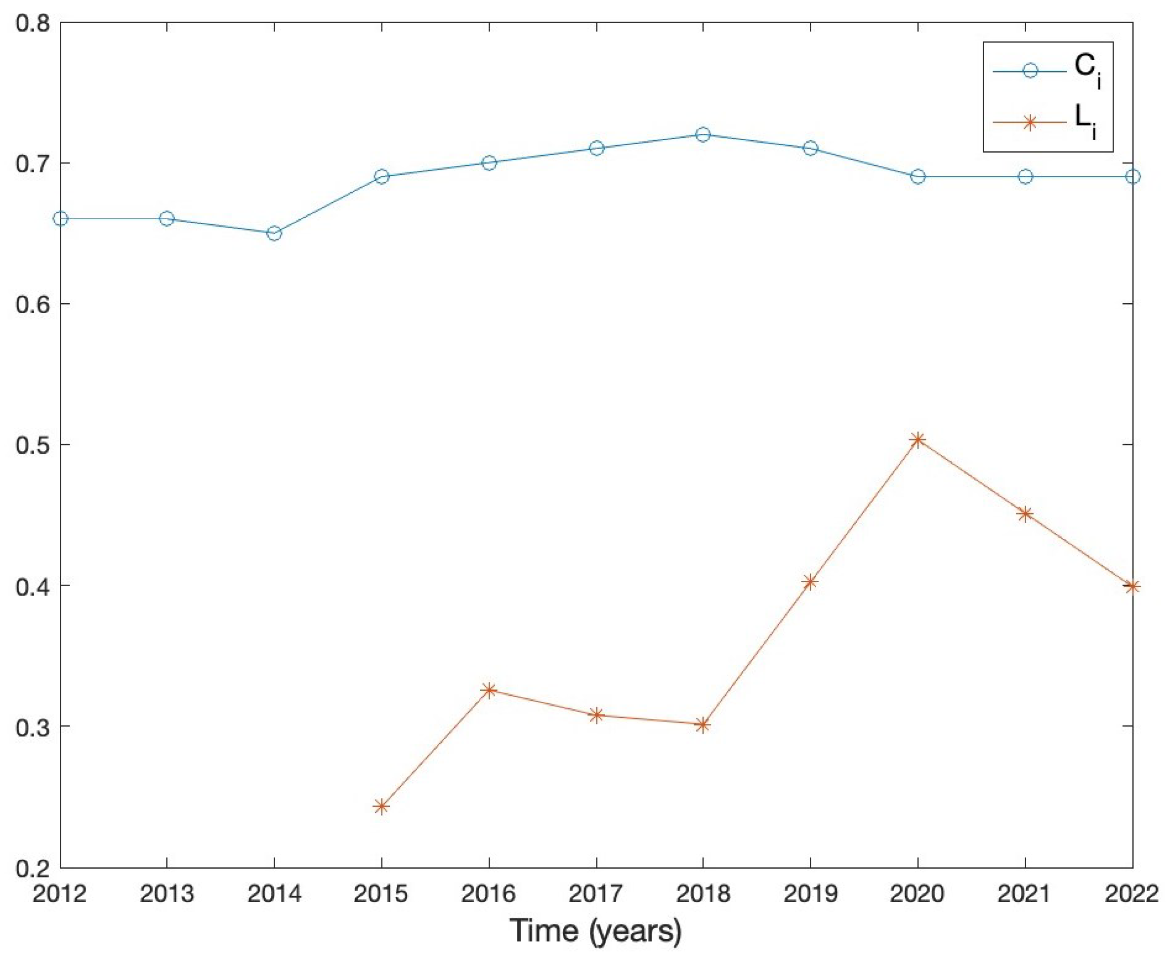
Figure 1. Graph of data C i and L i , which are normalized complements of the CPI and IGI, respectively, taken from Table 1 and Table 2.
Mca 29 00081 g001
Figure 2. Numerical simulation of the solution of the model in differential equations for the CPI, Equations (3)–(5), with adjusted parameters, for four study scenarios: (a) A flexible projected level of P./low S., (b) a flexible projected level of P./high S., (c) a strict projected level of P./low S., and (d) a strict projected level of P./high S.
Mca 29 00081 g002
Figure 3. Numerical simulation of the solution of (b) the case of the model for the CPI for the scenario of (a) a flexible projected level of anticorruption P./low S.
Mca 29 00081 g003
Figure 4. Sensitivity analysis graph of the system of Equations (3)–(5), for all parameters.
Mca 29 00081 g004
Table 1. Corruption Perception Index for Mexico.
20122013201420152016201720182019202020212022
CPI3434353130292829313131
C i 0.660.660.650.690.700.710.720.710.690.690.69
Source: Transparency Internacional, CPI [24].
Table 2. Index of Global Impunity for Mexico.
20152016201720182019202020212022
IGI75.767.4269.2169.8449.6760.8
L i 0.24300.32580.30790.30160.40240.50330.45120.3992
Source: Scales of impunity around the world, Impunity Global Index [21].
Table 3. Estimated values of the parameters.
Case P./S. α β γ 1 γ 2 Error E ( p )
(a) Flexible/Low0.1150740426.370546550.177928239.231096060.0156558527
(b) Flexible/High0.101645486.552507230.146312989.491348490.0156262753
(c) Strict/Low0.096167416.618618400.132795619.585774490.0156320420
(d) Strict/High0.038802137.842294850.0126929011.358650770.0156322746
P. Policy, S. Sensitivity.
Disclaimer/Publisher’s Note: The statements, opinions and data contained in all publications are solely those of the individual author(s) and contributor(s) and not of MDPI and/or the editor(s). MDPI and/or the editor(s) disclaim responsibility for any injury to people or property resulting from any ideas, methods, instructions or products referred to in the content.