Enhanced Forecasting of Equity Fund Returns Using Machine Learning

Abstract

This paper aims to explore the integration of machine learning with risk and return performance measures, to provide a data-driven approach to identifying opportunities in equity funds. We built a dataset with 72 performance measures in the columns calculated for multiple periods ranging from 1 to 120 months. By shifting the values in the 1- and 3-month return columns, we created two new columns, aligning the data for the month t with the return for the month $t+1$. We categorized each row into one of three classes based on the mean and standard deviation of the shifted 1- and 3-month returns during the period. Based on cross-validated accuracy, we focused on the top three classifiers. As a result, the developed models achieved accuracy, recall, and precision values exceeding 0.92 on the test data. In addition, models trained on 1 year of data maintained predictive reliability for up to 2 months into the future, achieving precision above 90% in forecasting funds with 3-month returns above the average. Thus, this study highlights the effectiveness of machine learning in financial forecasting, particularly within the environment of the Brazilian equity market.

1. Introduction

Machine learning techniques excel at identifying patterns within large and intricate datasets that traditional statistical methods may overlook. This capability improves prediction accuracy and, in the financial context, may provide investors with actionable insights into market trends and movements.

Among the different assets, investment funds represent an important segment of the financial market and offer diverse opportunities for innovation through machine learning. Equity investing is widely seen as a way to diversify or seek higher returns, typically through funds that pool investor money to trade stocks, also known as equity securities.

Brazil is a major player in the global landscape of investment funds. Its dynamic and evolving market is characterized by diverse offerings and regulatory frameworks that shape investor participation and fund management strategies. Brazil has a population of more than 203 million inhabitants and, according to the World Bank [1], its real GDP grew by 2.9% in 2023 and is projected to increase by 1.7% in 2024. The country maintains robust macroeconomic fundamentals, including substantial international reserves, minimal external debt, a credible central bank, a resilient financial system, and flexible exchange rates. Under Brazilian legislation, equity funds are organized as pooled assets collectively owned by shareholders under a co-property structure. Despite lacking a corporate structure, these funds can assume obligations and take legal actions. Investors in Brazilian equity funds hold quotas or shares, which represent their co-investment in the fund’s assets. These shares entitle investors to proportional rights over the entire fund portfolio without granting direct ownership of the underlying assets [2].

Financial models like the Capital Asset Pricing Model (CAPM) assess the return of a fund on its systematic risk (beta) to determine whether it adequately compensates for exposure to market risk [3]. However, the CAPM’s simplified approach, focusing on a single risk–return relationship, fails to account for the complexities that financial markets present. In contrast, the Sharpe and Treynor indices provide more nuanced perspectives on risk–return trade-offs. Sharpe considers both systematic and unsystematic risks, while Treynor focuses solely on systematic risk. The different recommendations of these indices highlight the limitations of relying on individual performance measures to make informed investment decisions.

We explore the integration of machine learning with traditional risk and return performance measures to offer a data-driven approach to identify investment opportunities in equity funds available in the Brazilian market, serving the needs of both retail and institutional investors. Using daily historical fund prices, we calculated eight performance measures for multiple periods ranging from 1 to 120 months. From this, using the last trading day of each month, we built a dataset with 72 performance measures in the columns. We categorized each row into one out of three classes according to the mean and standard deviation of the shifted 1- and 3-month returns.

Relevant related works in the field explore return forecasting using panels that combine cross-sectional and time-series data or complex models for general development frameworks in diverse time windows and investment products [4,5,6,7]. However, such general models often face challenges because of significant variations in the data. On the other hand, by selecting from multiple machine learning models, we developed specialized models focused on equity funds. Addressing concerns about overfitting and poor out-of-sample performance highlighted in [8], machine learning models would require periodic retraining to adapt to changes, such as data drift, over time, especially when dealing with dynamic financial data.

In contrast to the existing literature, we begin with time-series data and reformulate the problem, typically modeled as a time-dependent phenomenon, into a time-independent classification task. Although each row in the dataset corresponds to an observation at a specific point in time, there is no temporal dependency between the rows, which allows the model to focus on patterns in the features without accounting for sequential order and use a cross-validation process to evaluate a model’s performance and detect overfitting. In addition, training a model with monthly values is advantageous because it reduces the required data, simplifying the computation. Moreover, this approach aligns with the typical behavior of equity fund investors, who are generally not high-frequency traders.

Finally, our classification models achieved accuracy, recall, and precision values that exceeded 92% in the test data. In addition, we demonstrate that classification models trained in one year of data retained their predictive reliability for up to two months into the future, achieving precision above 90% in forecasting funds with 3-month returns above the average. Furthermore, by inspecting feature importance, we found that the models showed a notable reliance on few risk-adjusted performance measures and shorter-term periods.

The remainder of this paper is organized as follows. Section 2 summarizes the literature review and Section 3 explains the data and the research methodology. Section 4 and Section 5 indicate the empirical results and the discussion part, and finally, Section 6 presents the conclusion.

2. Related Work

Recent research highlights significant advances in financial forecasting using machine learning and deep learning models. Selvamuthu et al. [9] employed an Artificial Neural Network (ANN) utilizing three algorithms: Levenberg–Marquardt (LM), scaled conjugate gradient (SGC), and Bayesian regularization. They used high-frequency and tick data to predict trends in the Indian stock market. Asere and Nuga [10] demonstrated the effectiveness of LSTM and other machine learning techniques in predicting stock indices and improving investment decision-making. In addition, the performance of LSTM in forecasting cryptocurrency prices was evaluated, highlighting the effectiveness of deep learning in predicting financial stability [11]. Wade [12] explored the integration of traditional investment approaches with generative AI and deep learning models such as Transformers. Kouki [13], Li et al. [14] focused on predicting hedge fund returns and risk of stock price crashes using machine learning, underscoring the broad applicability of these technologies in various financial contexts.

Furthermore, research by Lee and Hsieh [15] focuses on predicting the relative performance of stocks within the S&P 500 index using machine learning to identify which stocks are likely to outperform others, providing valuable insights for portfolio management. Raza and Akhtar [16] used SVM, LSTM, ANN, and Random Forest models and 27 technical indicators to classify stock price movements, identifying % R, Momentum and Disparity 5 as critical predictors in all models. They recommend using hybrid approaches to incorporate real-time data for better decision-making in financial markets.

With the exponential growth of the Internet, the use of financial news and performance metrics has become a topic of increasing interest to improve equity market predictions. In a review [17], various data mining methods commonly employed in financial data analysis are summarized. The authors examine the advantages, limitations, and applications of these methods, including decision trees, support vector machines, Bayesian models, and others, emphasizing their strengths and applicable scenarios. Furthermore, Agrawal and Adane [18] introduced an algorithm designed to predict the NIFTY index on the Indian National Stock Exchange. This research integrated data from social networks, global market performance, news, and historical data to improve prediction accuracy. Comparative analysis showed that this method outperformed other machine learning algorithms in terms of accuracy.

Integrating advanced algorithms and feature engineering underpins contemporary stock market prediction models, as demonstrated by the reviewed studies, which showcase how these elements synergize to improve predictive accuracy. For example, the use of the Gradient Boosting Machine (GBM) in conjunction with customized feature engineering, as highlighted by Nabi and Saeed [19], shows how fine-tuning the input features can significantly improve prediction performance. Similarly, the combination of a three-stage feature engineering process with the NSGA-II-RF algorithm, as in Anupama et al. [20], exemplifies the synergy between feature preparation and sophisticated modeling techniques. These integrated approaches not only enhance the robustness of stock price forecasts, but also pave the way for more innovative and effective financial prediction methodologies. Furthermore, Maldonado et al. [21] reviews various methods used to improve model inputs, exploring techniques such as statistical analysis, dimensionality reduction, and machine learning-based selection, which collectively highlight the diversity and critical role of feature engineering in financial predictions.

3. Methodology

3.1. Data Description and Data Preparation

Daily historical prices spanning 10 years were used to calculate various performance measures, including return, volatility, beta, tracking error, Sharpe ratio, Sortino ratio, information ratio, and Treynor index. These metrics, detailed in

Table 1. Featured abbreviations and mathematical expressions.

$R_{i,t}=\frac{P_{i,t}-P_{i,t-1}}{P_{i,t-1}}$
${\sigma }_{i,t}=\sqrt{{\displaystyle \frac{1}{N-1}}{\sum }_{t=1}^N{(R_{i,t}-\overline{R_i})}^2}$
${\beta }_{i,t}={\displaystyle \frac{\mathrm{Cov}(R_{i,t},R_b)}{\mathrm{Var}\left(R_b\right)}}$
${\mathrm{TE}}_{i,t}=\sqrt{{\displaystyle \frac{1}{N}}{\sum }_{i=1}^N{(R_{i,t}-R_b)}^2}$
${\mathrm{SHR}}_{i,t}={\displaystyle \frac{\overline{R_i}-R_f}{{\sigma }_{i,t}}}$
${\mathrm{SOR}}_{i,t}={\displaystyle \frac{\overline{R_i}-R_f}{{\sigma }_{di,t}}}$
${\mathrm{IR}}_{i,t}={\displaystyle \frac{\overline{R_i}-R_b}{{\mathrm{TE}}_{i,t}}}$
${\mathrm{TI}}_{i,t}={\displaystyle \frac{\overline{R_i}-R_f}{{\beta }_{i,t}}}$

$R_{i,t}$: return of the fund i on day t; $P_{i,t}$: price of the fund i on day t; $P_{i,t-1}$: price of the fund i on the previous day $t-1$; ${\sigma }_{i,j}$: standard deviation of the fund’s returns (volatility); N: number of observations (days); $\overline{R_i}$: average return of the individual in a period; $R_b$: return of the benchmark (IBOVESPA Index) in a period; $R_f$: the return on a risk-free asset (SELIC) in a period; $\mathrm{Cov}(R_i,R_b)$: covariance between the return of the individual stock and the market return, in this case, IBOVESPA index; $\mathrm{Var}\left(R_b\right)$: variance of the market return, in this case, IBOVESPA index; ${\mathrm{TR}}_{i,t}$: tracking error of the fund i on the day t; ${\mathrm{SHR}}_{i,t}$: Sharpe ratio of the fund i on day t; ${\mathrm{SOR}}_{i,t}$: Sortino ratio of the fund i on day t; ${\mathrm{TI}}_{i,t}$: Treynor index of the fund i on day t; ${\sigma }_{di,t}$: standard deviation of the downside (negative returns).

, are calculated according to standard financial methodologies [3].

For benchmarking, we use the IBOVESPA Index, which reflects the average performance of highly traded stocks on the São Paulo Stock Exchange, providing a gauge of the general performance of the Brazilian stock market [22]. The Selic rate, which serves as the reference interest rate in Brazil, represents the return on a risk-free asset within the Brazilian economy [23]. Together, these benchmarks offer essential points of comparison for evaluating the risk-adjusted returns of the funds studied.

Using daily data, we computed the performance measures in Table 1 for each fund over nine different time intervals (1, 3, 6, 12, 24, 36, 48, 60, and 120 months), totaling 72 distinct measures. To approximate monthly periods while using daily data, we employed time intervals that are multiples of 21 days, assuming 21 trading days in a month and 252 in a year. Equity fund performance measures are also accessible through various online platforms and financial databases [24].

3.1.1. Aggregating Daily Data into Monthly Intervals

Although daily data were available for all measures listed in Table 1, only end-of-month values for each fund were used. Training a model with monthly values is advantageous because it reduces the required data and simplifies the computation. Furthermore, this approach aligns with the typical behavior of equity fund investors, which are generally not high-frequency traders, especially considering that the volatility of these funds is typically lower compared to other investment options.

This study focuses on equity funds registered with the Brazilian Securities and Exchange Commission (CVM), specifically equity funds with at least 100 shareholders. This criterion ensures that the selected funds are generally open to public investment rather than restricted, exclusive, or closed-end funds. By targeting widely accessible funds, the findings of this study are more relevant and applicable to a broader audience, particularly individual investors.

3.1.2. Data Transformation

We created two distinct datasets based on the two experiments proposed in this study. In one dataset, the 1-month return column is shifted, aligning the historical data for month t with the return data for month $t+1$. The second dataset was created using the same approach, but with the 3-month return column shifted. This transformation created time-lagged features that allowed comparisons between historical and future values within the dataset. An important consideration is that a fund must meet the criteria established in the previous filtering step (Section 3.1.1) for both the month t and the subsequent month $t+1$; otherwise, its data will be excluded from the analysis.

Table 2. An illustration of the process for creating the shifted returns columns in the dataset, which includes 72 performance measures of equity funds used as features for the machine learning models. The 1-month-shifted return column (highlighted in gray), named $R_{t+1}^{1M}$, is used in Section 3.2 to define the labels for the classification models. The process for creating $R_{t+1}^{3M}$ is the same and is not shown here.

		Return			Volatility			Beta			Track	Sharpe	Sortino	Info	Treynor
											Error	Ratio	Ratio	Ratio	Index
	Shifted
Date	1-M	1-M	3-M	⋯	1-M	3-M	⋯	1-M	3-M	⋯	⋯	⋯	⋯	⋯	⋯
23-01	−0.032	0.061	−0.003	⋯	0.402	0.399	⋯	1.295	1.125	⋯	⋯	⋯	⋯	⋯	⋯
23-02	−0.071	−0.032	0.002	⋯	0.361	0.387	⋯	1.174	1.214	⋯	⋯	⋯	⋯	⋯	⋯
23-03	0.131	−0.071	−0.045	⋯	0.309	0.336	⋯	0.927	1.044	⋯	⋯	⋯	⋯	⋯	⋯
23-04	0.092	0.131	0.036	⋯	0.334	0.333	⋯	0.920	1.007	⋯	⋯	⋯	⋯	⋯	⋯
23-05	0.190	0.092	0.145	⋯	0.300	0.315	⋯	0.791	0.893	⋯	⋯	⋯	⋯	⋯	⋯
23-06	0.049	0.190	0.470	⋯	0.376	0.333	⋯	1.290	0.979	⋯	⋯	⋯	⋯	⋯	⋯
23-07	0.060	0.049	0.363	⋯	0.286	0.314	⋯	1.339	1.087	⋯	⋯	⋯		⋯	⋯
23-08	0.078	0.060	0.284	⋯	0.233	0.299	⋯	1.155	1.236	⋯	⋯	⋯	⋯	⋯	⋯
23-09	0.003	0.078	0.199	⋯	0.222	0.245	⋯	0.236	0.926	⋯	⋯	⋯	⋯	⋯	⋯
23-10	0.069	0.003	0.164	⋯	0.371	0.280	⋯	0.194	0.604	⋯	⋯	⋯	⋯	⋯	⋯
23-11	0.036	0.069	0.156	⋯	0.228	0.281	⋯	0.179	0.327	⋯	⋯	⋯	⋯	⋯	⋯
23-12	0.083	0.036	0.111	⋯	0.221	0.280	⋯	1.157	0.420	⋯	⋯	⋯	⋯	⋯	⋯
24-01	−0.008	0.083	0.187	⋯	0.204	0.216	⋯	0.805	0.566	⋯	⋯	⋯	⋯	⋯	⋯
24-02	−0.068	−0.008	0.113	⋯	0.282	0.234	⋯	0.981	0.903	⋯	⋯	⋯	⋯	⋯	⋯

presents the structure of our dataset for a specific fund, highlighting the gray column where the 1-month return has been shifted relative to the original 1-month return. A similar operation is performed for the 3-month return.

Furthermore, in Section 3.2, these columns of 1- and 3-month-shifted returns are named $R_{t+1}^{1M}$ and $R_{t+1}^{3M}$, respectively, indicating that they represent returns at $t+1$, or 1 month ahead. After all these operations, the data from January 2023 to March 2024 are selected, yielding a dataset containing 4970 rows.

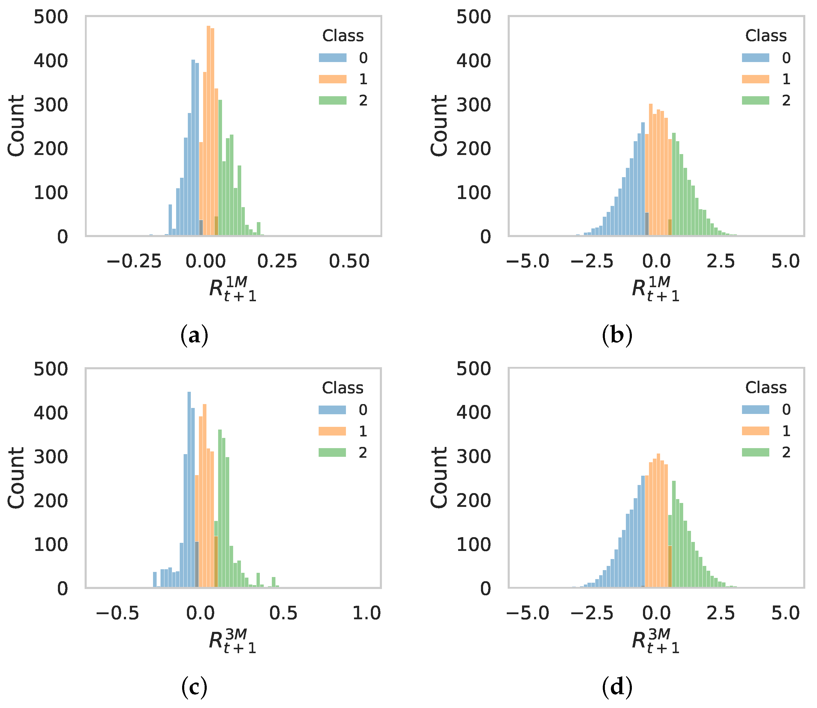
3.2. Labels Definition

Using the panel dataset containing 4970 observations, we define three categories based on the 1- and 3-month-shifted returns ($R_{t+1}^{1M}$ and $R_{t+1}^{3M}$). Labels for training the classification models employed are determined based on the average return (${\overline{R}}_{t+1}^{nM}$) and the standard deviation (${\sigma }_{t+1}^{nM}$) of $R_{t+1}^{1M}$ and $R_{t+1}^{3M}$. To ensure balanced subsets, the labels are assigned as follows.

$$\mathrm{Class}=\left\{\begin{array}{cc}0\hfill & \mathrm{if}{R}_{t+1}^{nM}\le {\overline{R}}_{t+1}^{nM}-0.5{\sigma }_{t+1}^{nM}\hfill \\ 2\hfill & \mathrm{if}{R}_{t+1}^{nM}\ge {\overline{R}}_{t+1}^{nM}+0.5{\sigma }_{t+1}^{nM}\hfill \\ 1\hfill & \mathrm{otherwise}\hfill \end{array}\right.$$

(1)

3.3. Feature Engineering

Applying Equation (1) to the original data, the resulting dataset is fairly balanced between classes. The descriptive statistics of $R_{t+1}^{1M}$ and $R_{t+1}^{3M}$ are presented in

Table 3. Descriptive statistics for classes 0, 1, and 2 for $R_{t+1}^{1M}$.

	Data	Class 0	Class 1	Class 2
count	4970	1683	1874	1413
mean	0.009669	−0.057537	0.012153	0.086422
std	0.063632	0.028733	0.016729	0.040091
min	−0.371327	−0.371327	−0.022107	0.041519
25%	−0.037126	−0.073548	−0.001007	0.056562
50%	0.008172	−0.050458	0.011537	0.080719
75%	0.048322	−0.036692	0.027170	0.106506
max	0.565069	−0.022210	0.041356	0.565069

and

Table 4. Descriptive statistics for classes 0, 1, and 2 for $R_{t+1}^{3M}$.

	Data	Class 0	Class 1	Class 2
count	4970	1623	1814	1533
mean	0.033659	−0.087063	0.029746	0.166100
std	0.116011	0.056746	0.032603	0.077302
min	−0.609930	−0.609930	−0.024153	0.091768
25%	−0.049681	−0.098293	0.002937	0.119454
50%	0.024955	−0.071773	0.027164	0.144124
75%	0.114138	−0.051058	0.056815	0.174111
max	1.004956	−0.024403	0.091638	1.004956

.

3.4. Model Setup

In this study, we assigned 80% (3976 rows) of the dataset to training and 20% (994 rows) to testing. We initialize the training environment and create the transformation pipeline using PyCaret, which was also used to evaluate different classifiers and their corresponding performance metrics. This library is specifically designed to simplify machine learning workflows by automating tasks such as data preprocessing, feature engineering, model selection, and deployment. In addition, it facilitates the visualization and comparison of various models. By default, the function compare_models applies a 10-fold cross-validation process, but this can be adjusted if needed. PyCaret also optimizes hyperparameters as part of its functionality, streamlining model selection and evaluation. In addition, we use feature transformation to enhance the model’s performance, specifically applying the quantile transformation available in PyCaret’s setup. This transformation modifies the features using quantiles, making their distribution more Gaussian-like (Figure 1). For each machine learning model assessed in our study, we compute the following performance metrics:

• Accuracy: The proportion of correct predictions out of all predictions.
• AUC (Area Under the Curve): A metric that summarizes the performance of a binary classifier in terms of the false positive rate (FPR) and the true positive rate (TPR).
• Recall: The proportion of positive instances that were correctly identified.
• Precision: The proportion of positive predictions that were actually positive.
• F1-score: The harmonic mean of precision and recall.
• Kappa: A metric that measures the agreement between the predictions of the model and the true labels, corrected for chance.
• MCC (Matthews Correlation Coefficient): A metric that balances the true positive rate and the false positive rate.
• Time (TT): The time taken to fit the model and make predictions.
• Confusion matrices: Show the actual versus predicted classifications for each class, including true positives, false positives, true negatives, and false negatives.

3.5. Computational Resources

All computation were executed on a Dell XPS 8940 workstation with the following specifications: CPU: Intel(R) Core(TM) i7-10700 CPU @ 2.90 GHz, 8 cores, 16 threads; memory: 16 GiB, DDR4-3200 MHz; video: GeForce RTX 3060; NVMe WDC 512 GB—Sandisk Corp., Milpitas, CA, USA; 22.04.2-Ubuntu 6.5.0-41-generic.

4. Results

Data from April and May 2024, which were not used during the training–testing phase, were employed as unseen validation data to assess the forecasting performance of the models.

The training set is processed through a PyCaret workflow that trains and evaluates the performance of 14 classifiers from the model library using cross-validation. The results, presented in

Table 5. Comparison of model performance for all models with general accuracy greater than 0.800 in predicting the 1-month return $R_{t+1}^{1M}$ classes. The accuracy results of other classifiers available in PyCaret, not shown in the table, were Ridge Classifier = 0.7965; Linear Discriminant Analysis = 0.7892; SVM–Linear Kernel = 0.7611; Ada Boost Classifier = 0.7457; Naive Bayes = 0.5408 and Dummy Classifier = 0.3770.

Model	Accuracy	AUC	Recall	Prec.	F1	Kappa	MCC	TT (Sec)
Light Gradient Boosting Machine	0.9218	0.9855	0.9218	0.9225	0.9217	0.8818	0.8822	353.3480
Random Forest Classifier	0.9160	0.9850	0.9160	0.9170	0.9161	0.8731	0.8735	0.2710
Extra Trees Classifier	0.9142	0.9851	0.9142	0.9150	0.9142	0.8704	0.8708	0.1890
Gradient Boosting Classifier	0.8911	0.9725	0.8911	0.8918	0.8909	0.8355	0.8360	2.3540
Quadratic Discriminant Analysis	0.8627	0.9383	0.8627	0.8638	0.8627	0.7928	0.7933	0.1410
K Neighbors Classifier	0.8599	0.9560	0.8599	0.8634	0.8598	0.7881	0.7898	0.3230
Decision Tree Classifier	0.8436	0.8812	0.8436	0.8445	0.8436	0.7636	0.7640	0.1650
Logistic Regression	0.8081	0.9133	0.8081	0.8082	0.8074	0.7105	0.7112	0.5070

and

Table 6. Comparison of model performance for all models with general accuracy greater than 0.800 in predicting the 3-month return $R_{t+1}^{3M}$ classes. The accuracy results of other classifiers available in PyCaret, not shown in the table, were Ada Boost Classifier = 0.7958; SVM–Linear Kernel = 0.7897; Linear Discriminant Analysis = 0.7920; Ridge Classifier = 0.7746; Naive Bayes = 0.6366; Dummy Classifier = 0.3649.

Model	Accuracy	AUC	Recall	Prec.	F1	Kappa	MCC	TT (Sec)
Extra Trees Classifier	0.9253	0.9879	0.9253	0.9259	0.9251	0.8878	0.8882	0.1980
Light Gradient Boosting Machine	0.9250	0.9880	0.9250	0.9254	0.9249	0.8874	0.8877	341.5240
Random Forest Classifier	0.9210	0.9868	0.9210	0.9214	0.9209	0.8813	0.8816	0.3060
Gradient Boosting Classifier	0.9039	0.9778	0.9039	0.9047	0.9037	0.8556	0.8561	2.4840
Quadratic Discriminant Analysis	0.8727	0.9447	0.8727	0.8737	0.8728	0.8086	0.8090	0.1530
Decision Tree Classifier	0.8707	0.9020	0.8707	0.8714	0.8706	0.8056	0.8060	0.1880
K Neighbors Classifier	0.8644	0.9600	0.8644	0.8665	0.8641	0.7962	0.7975	0.3520
Logistic Regression	0.8287	0.9368	0.8287	0.8291	0.8284	0.7425	0.7430	0.5630

, show a score grid with the average cross-validated scores to predict the classification of the 1- and 3-month returns, $R_{t+1}^{1M}$ and $R_{t+1}^{3M}$, respectively.

Table 5 presents the performance metrics in predicting the 1-month return. The top three models, and their average cross-validated accuracy, are the Light Gradient Boosting Machine (LightGBM) (0.9218), Random Forest classifier (0.9160), and Extra Trees classifier (0.9142), evaluated on the test set. It should be noted that while the training time (TT) for the Random Forest and Extra Trees classifiers is less than 0.30 s, the LightGBM requires more than 353 s. When predicting the 3-month return, all models exhibit similar performance, with the Extra Trees performing slightly better overall. However, LightGBM again has significantly longer training times, as shown in Table 6.

We then refined our analysis by comparing the confusion matrices for the top three models (Figure 2 and Figure 3). Each matrix shows the actual versus predicted classifications for three classes (0, 1, and 2) for 1- and 3-month returns. In predicting the 1-month return, the true positive rate for class 2 is slightly lower than for the other classes. When predicting the 3-month return, the accuracy for classes 0 and 2 is better than for class 1, which is advantageous since these classes represent returns lower and higher than the average return, respectively.

4.1. Feature Importance

Feature importance measures how significantly each feature contributes to the accuracy or relevance of predictions in a classification task. Figure 4 and Figure 5 display the feature importance plots for predicting 1- and 3-month returns. For the 1-month return predictions, all three models rank ‘Return 1-M’ and ‘Sortino Ratio 1-M’ as the top features. In total, 16 features are highlighted as important features for at least one model. Taking into account all models, six characteristics are consistently significant, as shown in Figure 4d.

For 3-month return predictions, ’Return 1-M’ is the key feature for the LightGBM and Extra Trees, while the Random Forest classifier emphasizes ‘Sortino Ratio 1-M’. Taking into account all models, 15 main features appear (Figure 5d), with 7 common features among them.

4.2. Validation of Classifier Forecasts on Unseen Data

The top three models, LightGBM, Random Forest, and Extra Trees, are then validated on unseen data forecast for 1- and 3-month returns.

In the 1-month return forecast, for 1 month ahead (Figure 6), the prediction accuracy is generally low. Class 1 shows true positive rates ranging from 67.2% to 94%, while classes 0 and 2 exhibit significantly lower true positive rates, ranging from 17.3% to 52.2%. In general, the true positive rate for class 2 is higher than for class 0, with a maximum of 52.2% achieved by the Random Forest. When using the same models to forecast the 1-month return 2 months ahead, the performance deteriorates further, with classifiers achieving less than 10% true positives for classes 0 and 2. This means that the model is currently unable to forecast two months ahead and may need retraining to improve its ability.

In contrast, the 3-month return forecast for 1 and 2 months ahead (Figure 7) shows overall better results. There is an increase in true positives for classes 0 and 2, despite a decrease for class 1. Specifically, the Random Forest classifier achieves 85.4 % true positives for class 0 one month ahead and 77.2 % two months ahead. For class 2, the Extra Trees classifier performs better, with 21.5% true positives one month ahead and 35.8% two months ahead.

5. Discussion

We focus our discussion on the results of the 3-month return forecast, as it demonstrates superior performance compared to the 1-month return forecast. Additionally, we closely examine classes 0 and 2, which represent the extremes with the potential for significant losses if misclassified, since class 2 signifies gains above the average for the period, while class 0 indicates performance below the average.

Table 7. Summary of precision, recall, and F1-score for different classifiers’ predictions of 3-month returns for classes 0 and 2, 1 and 2 months ahead.

	Months Ahead	Model	Precision	Recall	F1-Score
Class 0	one	LightGBM	0.281	0.730	0.405
		Random Forest	0.330	0.854	0.475
		Extra Trees	0.297	0.820	0.434
	two	LightGBM	0.270	0.673	0.386
		Random Forest	0.300	0.772	0.433
		Extra Trees	0.277	0.525	0.361
Class 2	one	LightGBM	0.846	0.169	0.283
		Random Forest	0.750	0.185	0.297
		Extra Trees	0.824	0.215	0.341
	two	LightGBM	1.000	0.305	0.467
		Random Forest	0.938	0.316	0.472
		Extra Trees	0.944	0.358	0.519

summarizes the results for these classes in the 3-month return forecast. In the following sections, we discuss the performance of each classifier separately.

5.1. Random Forest Classifier

For class 0, Random Forest achieves the highest precision for both one and two months ahead, with values of 0.330 and 0.300, respectively. This indicates that Random Forest is the most reliable in correctly identifying class 0 instances with the fewest false positives. Extra Trees and LightGBM follow with slightly lower precision values, indicating that they are less reliable compared to the Random Forest for class 0.

5.2. Extra Trees Classifier

For the forecast for one month, Extra Trees achieves the best performance in class 2 with an F1 score of 0.341. For the forecast for two months ahead, Extra Trees maintains its superior performance in class 2 with an F1 score of 0.519. Across both one and two months ahead, Extra Trees consistently demonstrates the highest performance in class 2 when considering the F1-score, which balances precision and recall.

5.3. Light Gradient Boosting Machine

For the two-month forward forecast, LightGBM has the highest precision for class 2 at 0.846, indicating that this model is the most precise in identifying funds with returns above the average return. Extra Trees follows closely with a precision of 0.824, while Random Forest has the lowest precision at 0.75.

For the two-month-forward forecast, LightGBM achieves a perfect precision for class 2 of 1.0, meaning it perfectly identifies all instances it predicted as having above-average returns without false positives. The Extra Trees and Random Forest classifiers also perform well, with precisions of 0.944 and 0.938, respectively.

Additionally, LightGBM is the most reliable model for avoiding misclassifications from class 0 to class 2, since it did not misclassify any instances one and two months ahead. Random Forest and Extra Trees each had one misclassification from class 0 to class 2 two months ahead, indicating a minor issue but still fairly precise. The negative factor for LightGBM is that the TT is extremely high compared to the other two models.

5.4. Feature Importance

This analysis is important for understanding the model’s decisions and identifying which data features are most strongly associated with the different labeled classes. It also provides guidance for future data collection and feature engineering by highlighting the most informative features of the model. From Figure 4 and Figure 5, it is evident that the models are mainly based on performance measures for periods under 12 months. For both 1- and 3-month forecasts, the only longer-period performance measures identified as significant across all models are ‘Return 12-M’, ‘Sharpe Ratio 12-M’, and ‘Volatility 36-M’. This highlights the dependence of the models on recent data. Additionally, the models heavily rely on 1-month return, which in our framework represents the return at the end of the current month, along with the Sharpe and Sortino ratios, which are risk-adjusted metrics for evaluating investment performance—the Sharpe ratio assesses overall risk relative to risk-free returns, whereas the Sortino ratio focuses exclusively on downside risk. This can drive future research toward simplifying models by emphasizing some key risk-adjusted metrics and shorter time frames.

6. Conclusions

This paper explored the application of advanced machine learning techniques to predict and forecast the 1- and 3-month returns of equity funds using real data from the Brazilian Securities and Exchange Commission (CVM) for the period from January 2023 to May 2024.

The PyCaret framework was instrumental in facilitating the experimentation and deployment of machine learning models, streamlining the entire process from data preprocessing to model evaluation. Based on the average cross-validated accuracy of 14 classifiers, the LightGBM, Random Forest, and Extra Trees classifiers were explored and accurately forecasted, with more than 90% precision, funds with 3-month returns above the average. Overall, Random Forest excelled in forecasting below-average 3-month returns for 1 and 2 months ahead. In contrast, Extra Trees achieved the highest F1-scores, forecasting above-average 3-month returns. Although LightGBM required considerably longer training times, it provided the most accurate forecasts for above-average 3-month returns. Furthermore, the models demonstrate remarkable accuracy in predicting 3-month returns 1 and 2 months in the future, effectively distinguishing funds with above-average returns while minimizing misclassification between under-average and above-average return classes. Although not all top-performing funds were identified, the models successfully identified several of them whose returns were above the average while maintaining a low risk of misclassification.

In terms of feature importance, the models exhibited a strong dependence on few risk-adjusted performance metrics and shorter evaluation periods. This insight could guide future financial modeling efforts to optimize predictive frameworks by focusing on key performance measures and time horizons to align with market dynamics and investment strategies.

Future research could prioritize feature engineering to identify the most effective performance measures among those utilized in this study, thereby simplifying and improving the explainability of the models. In addition, models can be integrated with other data from equity funds, including cross-sectional data and performance measures, to create sophisticated algorithms to identify investment opportunities. Furthermore, integrating explainable machine learning techniques could improve the interpretability and usability of AI-driven investment strategies by clarifying the influence of each measure on predictions. Moreover, the lack of long-term monitoring for model evaluation is a limitation of this study, which we aim to address by first simplifying the models through feature engineering and later implementing automated retraining pipelines activated when performance metrics drop below a predefined threshold, ensuring ongoing reliability and adaptability. Finally, we consider these models valuable tools for analyzing market strategies and designing investment portfolios, enabling individual and institutional investors to mitigate losses and make well-informed financial decisions.

References

1. World Bank. Brazil Overview. Available online: https://www.worldbank.org/en/country/brazil/overview (accessed on 5 July 2024).
2. Apex-Brasil. Legal Structure-VCPE Funds in Brazil. Available online: https://www.apexbrasil.com.br/uploads/Legal%20Structure%20-%20VCPE%20Funds%20in%20Brazil.pdf (accessed on 12 July 2024).
3. Bodie, Z.; Kane, A.; Marcus, A. Investments, 13th ed.; McGraw-Hill Education: New York, NY, USA, 2024. [Google Scholar]
4. Lewellen, J. The Cross-section of Expected Stock Returns. Crit. Financ. Rev. 2015, 4, 1–44. [Google Scholar] [CrossRef]
5. Gu, S.; Kelly, B.; Xiu, D. Empirical Asset Pricing via Machine Learning. Rev. Financ. Stud. 2020, 33, 2223–2273. [Google Scholar] [CrossRef]
6. Zhou, Y.; Xie, C.; Wang, G.J.; Zhu, Y.; Uddin, G.S. Analysing and forecasting co-movement between innovative and traditional financial assets based on complex network and machine learning. Res. Int. Bus. Financ. 2023, 64, 101846. [Google Scholar] [CrossRef]
7. Kelly, B.; Malamud, S.; Zhou, K. The Virtue of Complexity in Return Prediction. J. Financ. 2024, 79, 459–503. [Google Scholar] [CrossRef]
8. Kelly, B.; Xiu, D. Financial Machine Learning. Found. Trends® Financ. 2023, 13, 205–363. [Google Scholar] [CrossRef]
9. Selvamuthu, D.; Kumar, V.; Mishra, A. Indian stock market prediction using artificial neural networks on tick data. Financ. Innov. 2019, 5, 16. [Google Scholar] [CrossRef]
10. Asere, G.; Nuga, K. Examining the Potential of Artificial Intelligence and Machine Learning in Predicting Trends and Enhancing Investment Decision-Making. Sci. J. Eng. Technol. 2024, 1, 15–20. [Google Scholar] [CrossRef]
11. Bouslimi, J.; Boubaker, S.; Tissaoui, K. Forecasting of Cryptocurrency Price and Financial Stability: Fresh Insights based on Big Data Analytics and Deep Learning Artificial Intelligence Techniques. Eng. Technol. Appl. Sci. Res. 2024, 14, 14162–14169. [Google Scholar] [CrossRef]
12. Wade, T. Transformers and Tradition: Using Generative AI and Deep Learning for Financial Markets Prediction. Ph.D. Thesis, London School of Economics and Political Science, London, UK, 2024. [Google Scholar]
13. Kouki, F. Design of Single Valued Neutrosophic Hypersoft Set VIKOR Method for Hedge Fund Return Prediction. J. Int. J. Neutrosophic Sci. 2024, 24, 317. [Google Scholar] [CrossRef]
14. Li, Y.; Xue, H.; Wei, S.; Wang, R.; Liu, F. A Machine Learning Approach for Investigating the Determinants of Stock Price Crash Risk: Exploiting Firm and CEO Characteristics. Systems 2024, 12, 143. [Google Scholar] [CrossRef]
15. Lee, T.H.; Hsieh, W.Y. Forecasting relative returns for SP 500 stocks using machine learning. Financ. Innov. 2024, 10, 45. [Google Scholar]
16. Raza, H.; Akhtar, Z. Predicting stock prices in the Pakistan market using machine learning and technical indicators. Mod. Financ. 2024, 2, 46–63. [Google Scholar] [CrossRef]
17. Liu, H.; Huang, S.; Wang, P.; Li, Z. A review of data mining methods in financial markets. Data Sci. Financ. Econ. 2021, 1, 362–392. [Google Scholar] [CrossRef]
18. Agrawal, L.; Adane, D. Improved Decision Tree Model for Prediction in Equity Market Using Heterogeneous Data. IETE J. Res. 2021, 69, 6065–6074. [Google Scholar] [CrossRef]
19. Nabi, K.; Saeed, A. A Novel Approach for Stock Price Prediction Using Gradient Boosting Machine with Feature Engineering (GBM-wFE). Kirkuk J. Appl. Res. 2020, 5, 259–275. [Google Scholar] [CrossRef]
20. Anupama, K.; Khandelwal, A.; Mohapatra, D.P. Prediction of stock price movement using an improved NSGA-II-RF algorithm with a three-stage feature engineering process. PLoS ONE 2023, 18, e0287754. [Google Scholar]
21. Maldonado, S.; Lopez, J.; Izquierdo, J. Survey of feature selection and extraction techniques for stock market prediction. Financ. Innov. 2022, 8, 41. [Google Scholar]
22. B3. IBOVESPA. Available online: https://www.b3.com.br/en_us/market-data-and-indices/indices/broad-indices/ibovespa.htm (accessed on 7 November 2024).
23. do Brasil, B.C. Taxa SELIC. Available online: https://www.bcb.gov.br/en/monetarypolicy/selicrate (accessed on 7 November 2024).
24. Retorno, M. Mais Retorno-Informações e Análises Financeiras. Available online: https://maisretorno.com/ (accessed on 7 November 2024).
Figure 1. Comparison of original and transformed datasets for feature targets R t + 1 1 M and R t + 1 3 M —(a,c) show the original dataset before any transformation, while (b,d) display the dataset after applying the quantile transformation, illustrating how the feature distributions have been adjusted to be more Gaussian-like. (a) Original, (b) transformed, (c) original, (d) transformed.
Mca 30 00009 g001
Figure 2. Confusion matrix on test data for the three classifiers with general accuracy greater than 0.800 in predicting the 1-month return R t + 1 1 M classes. Overall, the models find an 86.6–92.0% TP rate for classes 0 and 2 and an 89.3–90.7% TP rate for class 1. (a) LightGBM, (b) Random Forest, (c) Extra Trees.
Mca 30 00009 g002
Figure 3. Confusion matrix on test data for the three classifiers with general accuracy greater than 0.800 in predicting the 3-month return R t + 1 3 M classes. Overall, the models find a 93.2–95.7% TP rate for classes 0 and 2 and an 87.3–88.7% TP rate for class 1. (a) LightGBM, (b) Random Forest, (c) Extra Trees.
Mca 30 00009 g003
Figure 4. Feature importance for different classifiers’ predictions of 1-month return. (a) LightGBM, (b) Random Forest, (c) Extra Trees, (d) Features ranked among the top 10 in importance across all classifiers.
Mca 30 00009 g004
Figure 5. Feature importance for different classifiers’ predictions of 3-month return. (a) LightGBM, (b) Random Forest, (c) Extra Trees, (d) features ranked among the top 10 in importance across all classifiers.
Mca 30 00009 g005
Figure 6. Confusion matrices for different classifiers’ forecasts of 1-month return on unseen data: Comparison of 1 and 2 months ahead. (a) LightGBM (one month ahead), (b) Random Forest (one month ahead), (c) Extra Trees (one month ahead), (d) LightGBM (two months ahead), (e) Random Forest (two months ahead), (f) Extra Trees (two months ahead).
Mca 30 00009 g006
Figure 7. Confusion matrices for different classifiers’ forecasts of 3-month return on unseen data: comparison of 1 and 2 months ahead. (a) LightGBM (one month ahead), (b) Random Forest (one month ahead), (c) Extra Trees (one month ahead), (d) LightGBM (two months ahead), (e) Random Forest (two months ahead), (f) Extra Trees (two months ahead).
Mca 30 00009 g007