Abstract
Biological research traditionally relies on experimental methods, which can be inefficient and hinder knowledge transfer due to redundant trial-and-error processes and difficulties in standardizing results. The complexity of biological systems, combined with large volumes of data, necessitates precise mathematical models like ordinary differential equations (ODEs) to describe interactions within these systems. However, the practical use of ODE-based models is limited by the need for curated data, making them less accessible for routine research. To overcome these challenges, we introduce LazyNet, a novel machine learning model that integrates logarithmic and exponential functions within a Residual Network (ResNet) to approximate ODEs. LazyNet reduces the complexity of mathematical operations, enabling faster model training with fewer data and lower computational costs. We evaluate LazyNet across several biological applications, including HIV dynamics, gene regulatory networks, and mass spectrometry analysis of small molecules. Our findings show that LazyNet effectively predicts complex biological phenomena, accelerating model development while reducing the need for extensive experimental data. This approach offers a promising advancement in computational biology, enhancing the efficiency and accuracy of biological research.
1. Introduction
Traditionally, biological research has been dominated by experimental methods, which often rely on descriptive techniques for communication and knowledge transfer. These approaches have led to challenges in standardizing results, generating redundant experiments, and increasing costs. To overcome these limitations, there has been a growing emphasis on integrating mathematical modeling into biological research, particularly through the use of ordinary differential equations (ODEs) to articulate complex biological phenomena. ODEs conceptualize variables with their derivatives structured as equations that incorporate biological interactions. This modeling facilitates detailed predictions of biosystem states, allowing common experimental interventions such as inhibition or overexpression to be modeled as modifications to initial conditions.
Despite their utility, ODEs encounter substantial challenges in modeling biological systems both accurately and efficiently. A pivotal issue is the integration of experimental data into ODE models, a process that traditionally requires extensive input from biomathematicians in areas such as text mining, data curation, and empirical equation development [1]. These models often suffer from a lack of standardization and are slow to integrate new discoveries, thereby constraining their utility in biological research.
Recent advancements in differential equation modeling within physics and mathematics have significantly influenced the field of biological modeling. The sheer diversity and volume of biological data make it an excellent candidate for these advanced methodologies. Beginning in 2009, pioneers such as Michael Schmidt and Hod Lipson utilized computational techniques to derive equations directly from experimental data [2]. This trend was advanced in 2018 when Ricky Chen incorporated maximum likelihood estimation with ODE solvers into neural networks, further refined by John Qin’s application of these techniques within the Residual Network (ResNet) framework and Samuel Kim’s introduction of symbolic dictionaries for equation discovery [3,4,5]. Chen, Liu, and Sun extended this line of work by integrating autograd differentials into the networks, enhancing the physics-informed learning from sparse data [6]. Although categorized under symbolic regression, these methods demand substantial datasets even for relatively simple differential equation systems and significant computational resources, which restrict their practical application in biological research.
Alternative methods for ODE approximation often rely on mathematical tools like neural ODE solvers and spline functions. Latent ODE models use neural ODE solvers triggered at model-determined times, offering strong approximation power but lacking interpretability and transferability due to their empirical nature [7,8,9]. RNNs (recurrent neural networks) not only show similar behavior, updating internal states over time, but also fall short in providing meaningful mechanistic insights [10,11,12,13]. Spline functions are flexible and smooth but require many parameters, leading to large, slow models [13,14,15,16]. Alex Liu introduced Kolmogorov–Arnold Networks (KANs), which use spline-based encoding to reduce model depth and parameter count [17]. However, KANs remain computationally expensive and time-consuming.
To address these biological and computational challenges, we developed LazyNet. This innovative model uses logarithmic and exponential functions embedded within the weights of a ResNet architecture to approximate ODEs through the Euler method. Supporting a broad spectrum of mathematical operations—including addition, subtraction, multiplication, division, exponentiation, and Taylor series expansions—LazyNet simplifies the complexities associated with spline functions and sidesteps the limitations of symbolic regression methods. Requiring fewer resources, LazyNet operates effectively with datasets under 30,000 samples on standard computation clusters.
In this study, LazyNet has been rigorously tested across various biological applications, including the dynamics of HIV populations, gene regulatory networks (GRNs), and the analysis of small molecule mass spectrometry (MS) [18,19,20,21]. These tests have confirmed that models trained with LazyNet can effectively assimilate and predict biological processes, demonstrating its capability and practicality in constructing ODE models for biosystems.
2. Materials and Methods
2.1. Model Layout
Consider a biosystem where the state of the system at any given point is dependent on its preceding state, forming a continuous sequence defined by a differential equation that reflects the intrinsic nature of the system’s interactions.
Let the sequence of states be represented as , , , …, where denotes the initial state of the system and denotes the state at the next time step, and so forth. Each state in this sequence evolves according to function F, which is consistent across the system and encapsulates the biological interactions. Using Euler’s method for the approximation of these dynamics, the progression of states can be mathematically modeled:
where denotes the time step increment, and represents the state at the subsequent time point. Each state encompasses the conditions of variables such as x, y, z, …, allowing for an iterative computation where each subsequent state is derived directly from its predecessor.
System F, plays a critical role in the sequential transition from state to within biological models. It encapsulates the inherent biological interactions and mechanisms, serving as a fundamental component in understanding the system’s dynamics, such as gene X’s influences over gene Y. The concept of data-driven discovery of ODE governing equations aims to automate the formulation of F using large datasets.
In LazyNet, this formulation is achieved:
where F is the ODE system built by LazyNet, it sums all the gene interactions defined or coded by weight matrix and , and bias .
From the entire network layout, the logarithmic and exponential layers are served as residue blocks (Figure 1). At the end of the network, an additional layer integrates these transformations with the current state and outputs the next state, meanwhile completing Residual Networks (ResNet) and Euler structures.
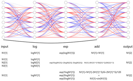
Figure 1.
Schematic architecture of the framework of LazyNet. LazyNet’s unique design approximates ODEs within a ResNet framework using logarithmic and exponential transformations. The diagram highlights the main components of LazyNet, including its dynamic weight adjustment capabilities, simplified mathematical operations through log and exp functions, and the integration of these elements into the output.
Figure 1 illustrates examples corresponding to the operations described in Equation (2). In the figure, N1[1] represents the initial data point of variable N1, while N1[2] indicates the subsequent data point, serving as the predicted output. Variables N2 and N3 denote additional variables within the dataset.
For instance, when no transformation is needed, setting w = 1 results in the following equation:
When representing more complex mathematical operations, such as multiplication and division, the weighted log-exp transformation can succinctly encode these interactions. For example, if = 1, = 2, = 3:
Similarly, complex functions, including trigonometric operations, can be approximated through polynomial expansions, such as the Taylor series:
Following the Euler method of ODE approximation, these encoded transformations are integrated into the residual structure of LazyNet to predict the subsequent state N1[2]:
By adjusting the weights and biases within each residual block, LazyNet flexibly represents a wide array of biological interactions, accurately capturing complex dynamics inherent in biological systems.
Despite the strengths of LazyNet, traditional modeling methods exhibit several limitations, motivating the development of LazyNet’s innovative design. Traditional modeling methods, such as recurrent neural networks (RNNs) and neural ordinary differential equations (Neural ODEs), predominantly rely on mathematical optimization without explicit biological mechanisms [7,8,9,10,11,12,13]. For instance, RNNs utilize gating mechanisms to control state transitions, artificially deciding which features activate or deactivate based solely on prior states, rather than realistic biological cues. Similarly, Neural ODEs invoke ODE solvers at empirically chosen points determined by mathematical heuristics, lacking direct biological reasoning. Such purely empirical approaches reduce interpretability and hinder knowledge transfer to different biological contexts.
Spline-based methods and symbolic regression present additional challenges [13,14,15,16]. Spline models use piecewise polynomial approximations, which rapidly increase complexity and parameter count as systems become more intricate, leading to computational inefficiency and difficulties in extracting meaningful insights. Symbolic regression, meanwhile, explores large spaces of mathematical expressions, typically yielding complicated equations that, despite fitting data accurately, lack straightforward biological interpretation and incur substantial computational costs.
In contrast, LazyNet effectively addresses these limitations through its simplified yet powerful architecture. By explicitly encoding biologically relevant interactions using log-exp transformations within a residual framework, model complexity is substantially reduced, and interpretability is enhanced by closely reflecting biological processes. Additionally, the residual design facilitates stable and computationally efficient training processes, supporting scalability for handling larger and more complex datasets. The result is a robust modeling approach capable of both accurate predictions and meaningful biological interpretation, overcoming the traditional trade-offs between computational efficiency, interpretability, and biological realism.
2.2. Training
During the training process, LazyNet takes each state from the training dataset as input and predicts the subsequent state, comparing this prediction to the ground-truth value. If the provided training samples sufficiently represent variability, LazyNet approximates a unique, optimal set of underlying ordinary differential equations (ODEs). Generally, the accuracy and generalization capabilities of the model improve with increasing diversity of training samples and the temporal span covered by the dataset. Ideally, the training dataset would encompass all potential variations and future scenarios, extending over a sufficient duration to comprehensively capture the system dynamics.
where V is the variety of the training samples and T is the time coverage for the training dataset. is the model learned by LazyNet, and is ground-truth governing equations.
From the perspective of ODE theory, system evolution follows a Markov process, meaning that the future state depends only on the current state and not on the sequence of past states. Mathematically, this can be represented as Equation (1) mentioned above.
This Markovian property allows a minimal batch size of two—capturing transitions between two consecutive time points—to theoretically suffice for approximating the governing equations. However, such minimal batches primarily emphasize local dynamics and may lead to overfitting on fine-grained variations, failing to capture broader system behavior. Conversely, overly large batch sizes may smooth out important transitions and dilute meaningful temporal changes, making it difficult for the neural network to detect dynamic clues and effectively learn the underlying mechanisms. In such cases, the model may converge poorly or not at all due to the lack of informative gradients.
By integrating L1 regularization, LazyNet is designed to provide the most parsimonious approximation of biological systems. For example, if two polynomial terms are sufficient to approximate a sine function, LazyNet will avoid using an unnecessary third term, showcasing its “lazy” yet effective design principle.
Overall, the practical training process can be written as a loss function as follows:
where w is the learnable weight, b is the batches to the last batch B, the training is based on each point n within batch b, and is the L1 regularization.
2.3. Data Preparation
2.3.1. Synthetic Data Studies
Both the HIV population and gene regulatory network (GRN) experiments were conducted using synthetic data [18,19]. The governing equations for each system were obtained from the published literature and implemented in MATLAB. Training and test datasets were generated programmatically.
For training, datasets were created by simulating trajectories from a range of initial conditions, each evolved across 500 time points using ODE solvers. These training conditions included multiple perturbations to initial states, enabling the model to learn a broad spectrum of system responses. For evaluation, test datasets were generated using completely unseen initial conditions—distinct from those used in training—to assess LazyNet’s ability to generalize. Full implementation scripts and dataset files are documented and accessible via the Data and Code Availability section.
2.3.2. Metabolite Data Study
The original literature aimed to predict metabolomic responses from proteomics data [21]. Due to data limitations—including unstructured, incomplete, or missing proteomics matrices—we refocused this study on predicting phenotypic behaviors using available metabolomics data alone.
The dataset included mass spectrometry profiles from eight engineered E. coli strains, each designed to produce one of three biochemical products. In total, 79 small molecules were profiled per strain, with one additional input feature representing time, making 80 input variables per sample. Although this study initially aimed to use over 100 experimental profiles, only 9 datasets were accessible in a usable format.
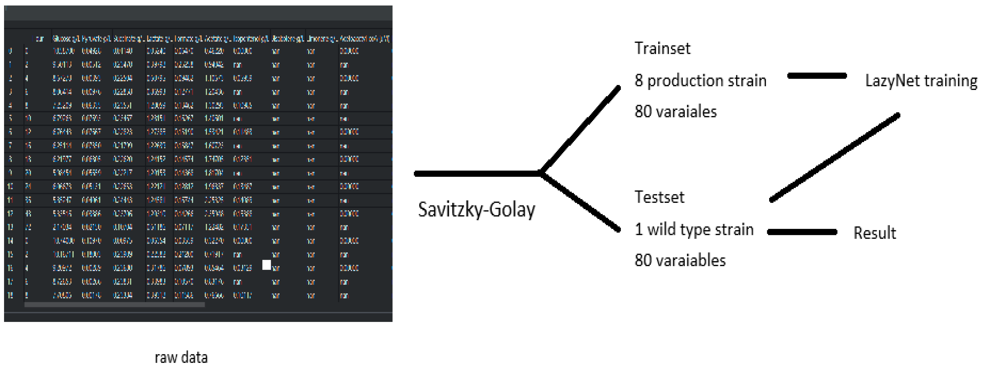
Each strain’s dataset originally included just 14 sparsely sampled time points. To enable ODE-based modeling, these were expanded to 500 time points using the Savitzky–Golay filter, improving temporal resolution. The wild-type strain was used for model validation. All datasets and processing scripts are included in the project’s GitHub repository and Figshare archive, as noted in the Data and Code Availability section.
2.3.3. Single-Cell RNA Sequencing (scRNA-seq)
The scRNA-seq data used in this study was derived from publicly available datasets investigating monocyte responses to LPS stimulation [20]. This dataset presented notable challenges for ODE modeling due to its high dimensionality, biological noise, and a limited cell count (~6000 cells across several time points).
Cells expressing fewer than 200 genes or with >5% mitochondrial RNA content were filtered out. PCA was used to identify 717 highly variable genes, which were used for downstream modeling. Clustering and trajectory inference were conducted using UMAP and ScVelo, respectively, and seven clusters were defined with associated pseudo-time scores. Gene expression trajectories along pseudo-time were extracted and smoothed using the Savitzky–Golay filter, expanding each sequence to 140 time points.
Because this task focused on extending trajectories rather than predicting new observations, no test set was constructed. All raw and processed data, along with scripts used for trajectory extraction and filtering, are available on GitHub and Figshare, as described in the Data and Code Availability section.
3. Results
3.1. LazyNet’s Estimation of HIV Strain ODE System
To assess the efficacy of LazyNet, we utilized a simplified biological model of HIV population dynamics articulated through 19 ordinary differential equations (ODEs). These equations, selected for their simplicity and absence of trigonometric or complex functions, aim to reduce baseline complexity.
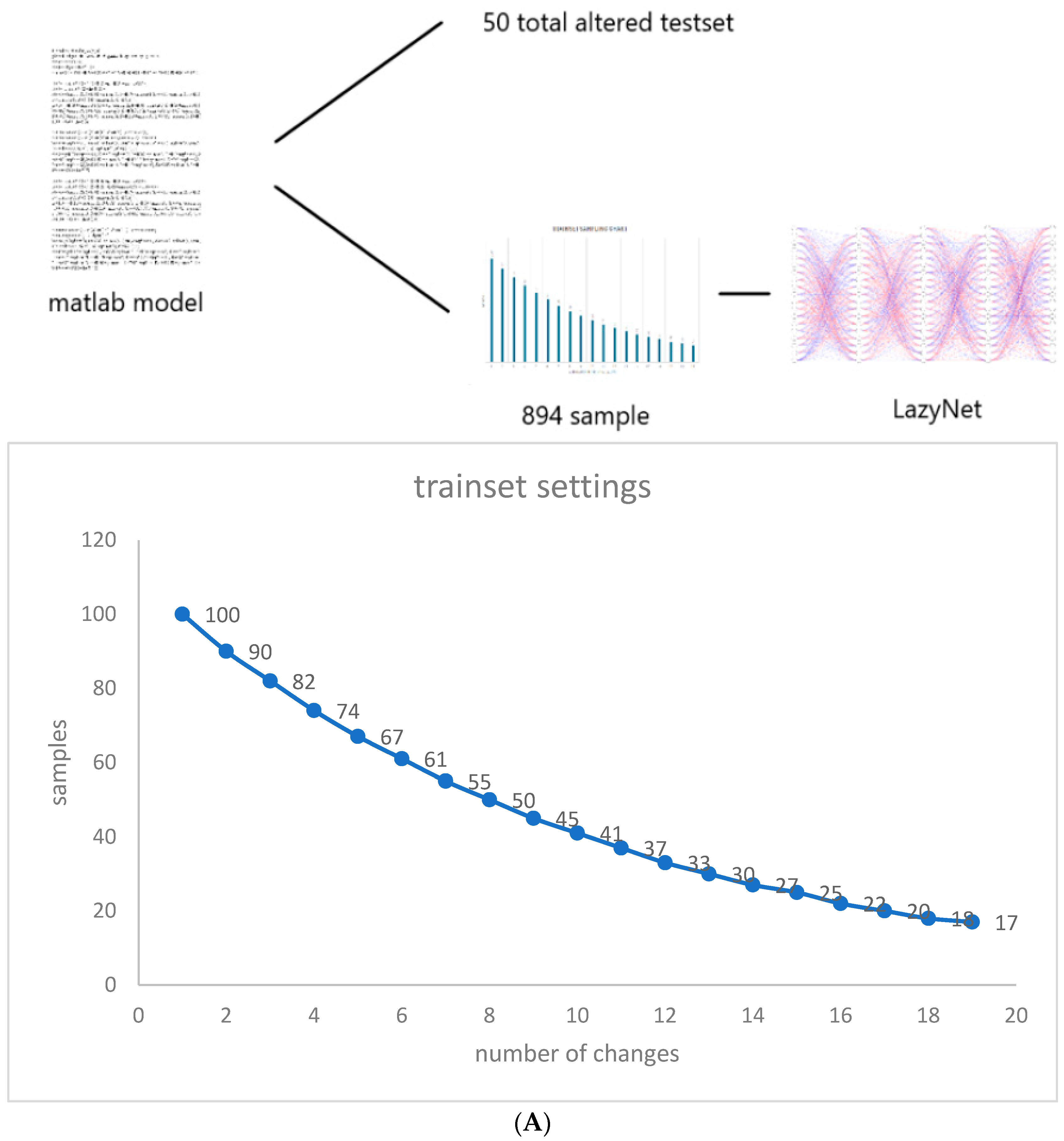
Considering the exploratory nature of this research and the unpredictable iterations required for validating LazyNet, we synthesized a dataset using MATLAB that mirrors typical variances found in virological studies, influenced by different initial infection populations. We began with 100 samples, each subjected to a unique random alteration in initial conditions. As the scenarios grew in complexity, the sample size was meticulously reduced to 894, analyzed across 500 temporal points (Figure 2A). For the testing phase, we crafted a dataset with random modifications to all initial values, through which we assessed LazyNet’s performance across 50 distinct test datasets (Figure 2B).

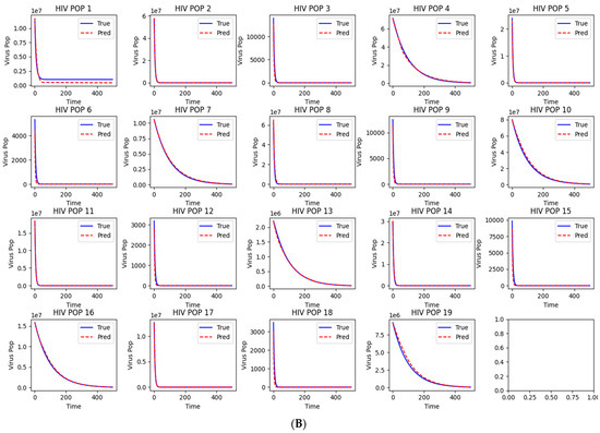
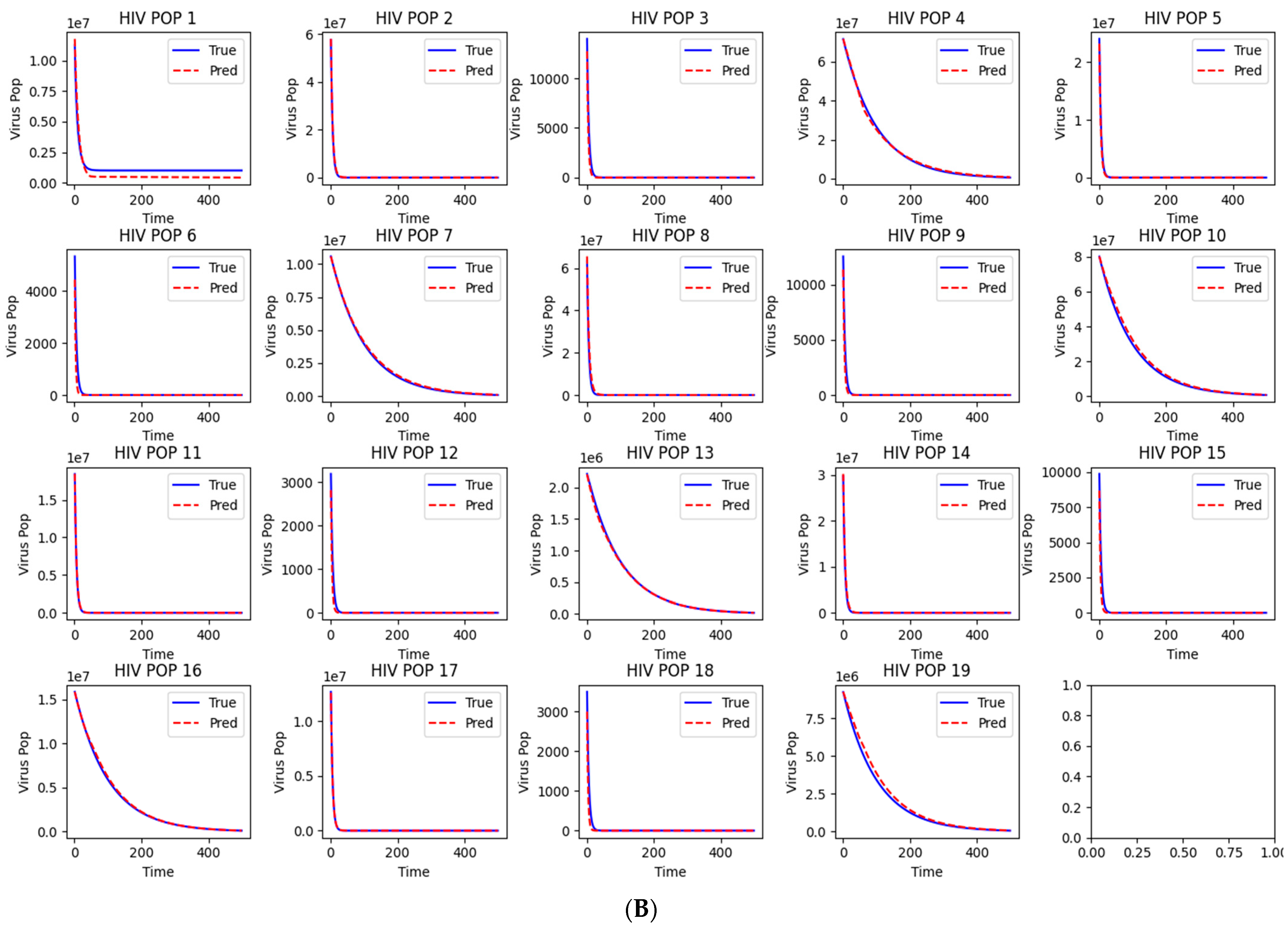
Figure 2.
Workflow and Results from LazyNet’s Evaluation on HIV Dynamics. (A) Trainset Sampling Chart showing the distribution of 894 samples, each uniquely altered in initial conditions. (B) Performance on 50 altered test datasets displayed through plots that compare LazyNet’s predictions (red lines) against expected outcomes based on the MATLAB model (blue lines). The result plot represents one of the test cases, and each subplot represents one strain.
The initial results are encouraging (Supplementary S1). LazyNet demonstrated a robust capacity to emulate the dynamic behaviors delineated by the ODE model, thereby validating its accuracy and fidelity. Upon preparing the synthetic dataset, we fine-tuned LazyNet to identify optimal training parameters within a few days—a notable enhancement over conventional manual modeling approaches. This improvement in training efficiency significantly streamlines the modeling process.
However, a limitation was observed in the dynamic range of the system. The generated dynamics were excessively stable, exhibiting very similar patterns despite variations in numerical values. This homogeneity points to a potential deficiency in LazyNet’s ability to accommodate more complex and dynamically varied scenarios. This finding underscores the need for further investigations with more intricate ODE systems to thoroughly evaluate LazyNet’s capabilities in modeling complex dynamic behaviors.
3.2. Adapting to Periodic Relationships in Gene Regulatory Networks (GRNs)
To explore LazyNet’s aptitude in managing intricate biological systems and interpreting periodic relationships, we applied it to a gene regulatory network (GRN) based on a model described in the established literature [19]. Omics-related data, which are pivotal in various biological studies, present a vast application scope for LazyNet. This is especially pertinent in experiments like gene knockouts or overexpression aimed at predicting the outcomes of physical experiments.
Our investigation employed a GRN model constituted by seven ordinary differential equations (ODEs) that mimic periodic biological functions similar to sine and cosine waves.
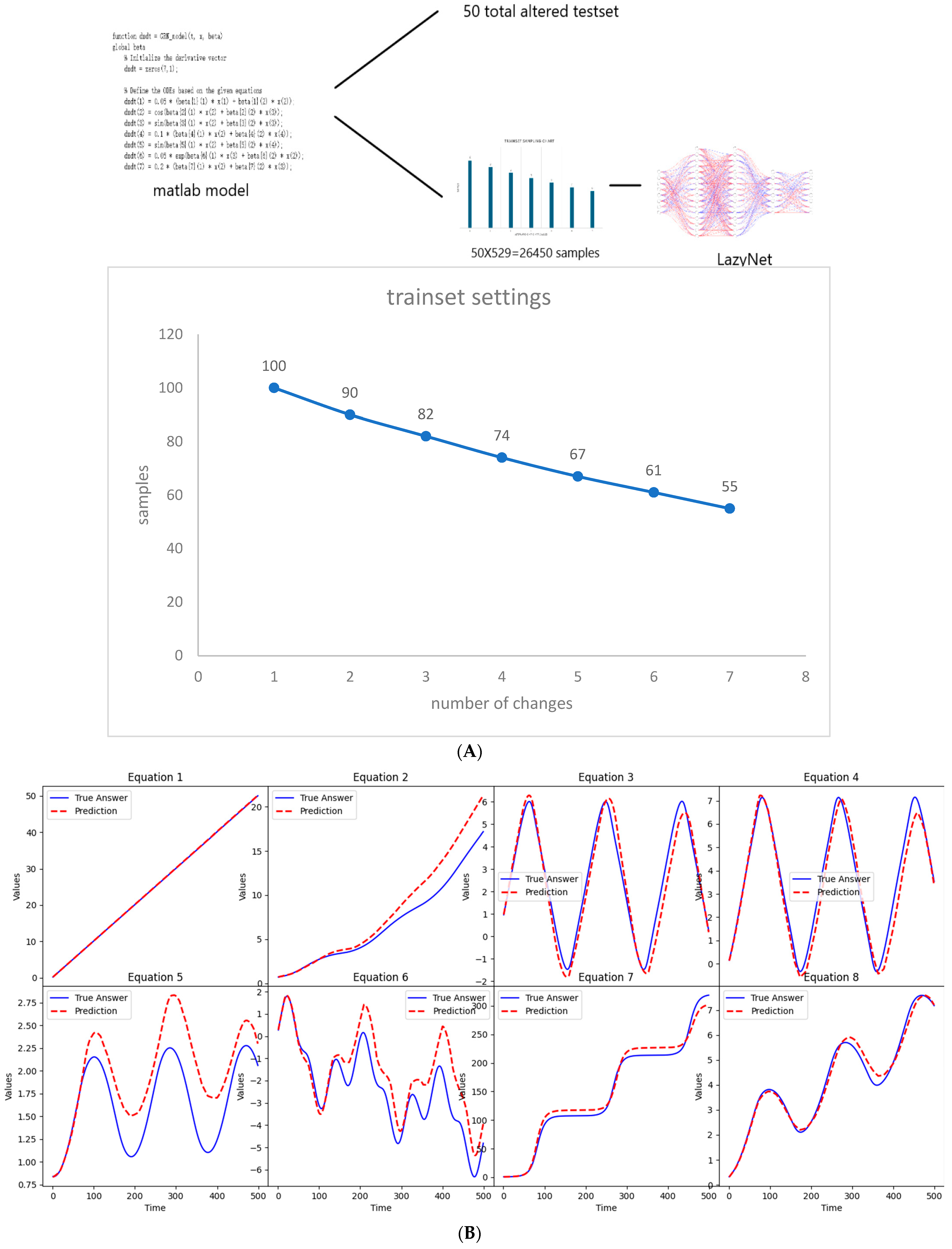
Synthetic data were generated using MATLAB, adhering to the methodological protocols previously described. This study commenced with 100 samples, each subjected to a random modification in initial conditions. As the complexity of the experiments increased, the sample size was judiciously reduced, culminating in 529 data points per set across 500 time points over 50 sets, totaling 26,450 samples (Figure 3A). The test set comprised 50 samples with altered initial conditions, presenting the model with unforeseen scenarios (Figure 3B and Supplementary S2). This design mirrors typical gene manipulation scenarios, such as knockouts and overexpression, providing a robust test of LazyNet’s capabilities in a controlled setting.
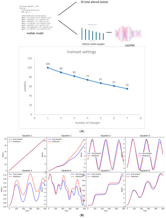
Figure 3.
Workflow and results from LazyNet’s evaluation on gene regulatory networks (GRNs). (A) Trainset sampling chart illustrating the distribution of 26,450 samples across 500 time points over 50 sets, each starting from 100 samples uniquely altered in initial conditions. (B) Performance on test datasets displayed through plots that compare LazyNet’s predictions (red lines) against expected outcomes based on the MATLAB model (blue lines). The result plot represents one of the test cases, and each subplot represents one strain.
The test involved 50 randomly selected samples, all of which were predicted with remarkable accuracy (Supplementary S2). These results not only confirm LazyNet’s precision but also underscore its vast potential in omics research. It enables researchers to predict the outcomes of physical experiments and pre-experimental planning. This capability is particularly beneficial in the fields of life sciences research and synthetic biology, where cost efficiency and experimental precision are paramount.
3.3. Real-World Data in Mass Spectrometry and Synthetic Biology
In this study, LazyNet was applied to mass spectrometry data from eight genetically modified E. coli strains, focusing on predicting phenotypic behaviors based on metabolomics data. Due to limited data availability and missing proteomics formats, the analysis was adapted to use only the accessible metabolomics profiles. Each dataset included 79 small molecules plus one time variable and was expanded to 500 points using the Savitzky–Golay filter to enhance resolution. This setting allowed us to evaluate LazyNet’s robustness under practical data constraints.
The results of our study, while encouraging, also highlight areas for further improvement. Among the 79 small molecules analyzed, 35 exhibited dynamic trends consistent with expected biological behavior (Figure 4A and Supplementary S3). This outcome reflects a common challenge in computational modeling—namely, that not all molecular data can be modeled. Notably, 24 of the molecules achieved a standardized RMSE below 1, indicating high predictive accuracy for a substantial portion of the dataset (Figure 4B). While the overall predictive performance remains moderate—likely limited by the small size and quality of the training data—this mirrors realistic scenarios in biological research, where data scarcity is a frequent constraint.
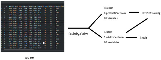
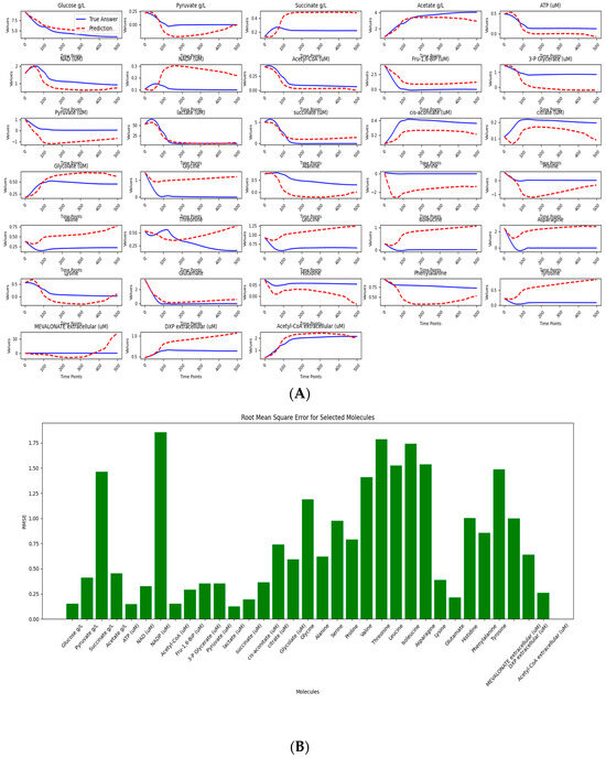
Figure 4.
Data processing and predictive analysis of E. coli strains mass spectrometry. The workflow begins with raw data, initially composed of 80 variables across 14 time points per set, processed using the interp1d function and Savitzky–Golay filtering to enhance data resolution. This refined data comprises the trainset and testset; the trainset covers eight productive strains, and the testset covers one wild-type strain. (A) depicts LazyNet’s predictive performance across various biochemical molecules, comparing LazyNet’s forecasts (red lines) to actual data (blue lines). (B) displays the root mean square error (RMSE) for each molecule across all time points.
Importantly, our approach successfully modeled a broader range of molecules compared to the original literature, which primarily focused on a smaller subset and likely reported only those with favorable results—far fewer than the 35 molecules identified here. In such contexts, LazyNet proves especially valuable by extracting actionable insights from suboptimal data, enabling data reuse, and supporting more comprehensive predictions.
A comparative analysis with the original study, which employed TPOT and reported a min–max scaled RMSE of 0.02 (standard deviation ~0.018) across 10 training datasets, helps contextualize LazyNet’s performance. TPOT (Tree-based Pipeline Optimization Tool) is an open-source AutoML library in Python that automates the selection and optimization of machine learning pipelines using genetic programming [22,23,24]. In other words, the original study evaluated a broad library of models and selected the best-performing pipeline to achieve their results. In contrast, our study achieved a scaled RMSE of 0.042, which is commendable given that our analysis was conducted using fewer datasets and was limited to metabolomics data—unlike the original study, which leveraged both proteomics and metabolomics data.
In this study, LazyNet achieved acceptable results under stringent conditions characterized by limited datasets and non-optimal data quality. The performance of LazyNet is commendable when compared to that of TPOT, especially considering that it utilized significantly fewer training datasets. Notably, LazyNet was not only able to extract meaningful insights from the data but also provided predictions that could be utilized for future research endeavors. These findings underscore the applicability of LazyNet in real-world scenarios, particularly in the fields of mass spectrometry data analysis and biosynthesis outcome prediction. The ability of LazyNet to yield practical results from limited data highlights its potential as a valuable tool in accelerating scientific discovery and enhancing decision-making processes in experimental biology.
3.4. Integrating LazyNet with scRNA-seq Data for Enhanced Trajectory Analysis
Single-cell RNA sequencing (scRNA-seq) represents one of the most advanced experimental techniques in biological research. A unique analysis enabled by scRNA-seq is RNA velocity, which uses RNA splicing dynamics to assign pseudo-time to cell states. This pseudo-time provides temporal information that is often scarce in other areas of biological research. The incorporation of LazyNet with RNA velocity analysis offers a novel approach to scRNA-seq data, enabling an unprecedented style of analysis. This integration provokes significant interest in employing LazyNet to harness the full potential of temporal data provided by RNA velocity, facilitating deeper insights into cellular dynamics.
In previous studies, RNA velocity provided by ScVelo indicated possible cyclic behaviors in monocytes—highlighted within a red rectangle in Figure 5A [20,25]. This behavior has been a topic of debate in earlier research focusing on the dominance of Ticam2 and Myd88 pathways. The sequencing data illustrated in Figure 5B captured a Ticam2-dominated phase (black arrow), where monocytes cycle back to a resting state following PBS exposure. However, activation of monocytes and related pathways, potentially involving Myd88, was not evident (red arrow).
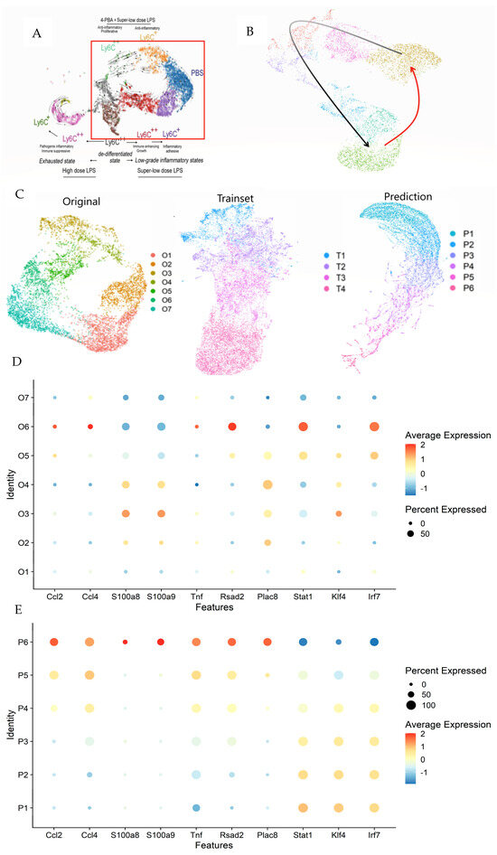
Figure 5.
Comprehensive analysis of monocyte dynamics using LazyNet and ScVelo. (A) UMAP visualization highlighting potential cyclic behaviors in monocytes, with the red rectangle indicating areas of interest. (B) The Ticam2 pathway (black arrows) denotes ScVelo and LazyNet trajectories (red arrow). (C) Comparison of UMAP clusters between original data, trainset, and LazyNet predictions, delineating shifts in cell state dynamics. (D) Dot plot representing differential expression levels in original data. (E) Dot plot representing differential expression levels in prediction.
LazyNet was utilized to extend the RNA velocity trajectory, facilitating an in-depth examination of the directionality and continuity of RNA velocity in monocyte populations. This approach enabled us to expand upon the foundational data, exploring cellular dynamics with greater precision.
Seurat was employed to analyze 717 genes identified by principal component analysis (PCA), which facilitated the creation of a robust Uniform Manifold Approximation and Projection (UMAP) [26]. The dataset was expanded to include 140 data points using the Savitzky–Golay filter for smoothing. The UMAPs for the original data, trainset, and predictions are depicted (Figure 5C and Supplementary S4), with the cluster names indicating the timeline. In contrast to initial expectations, the anticipated cyclic behavior in monocytes was not observed in the predictions. Extending this analysis further is deemed inappropriate as it would merely propagate the current dynamics without adding substantive insights and could likely introduce errors.
In the heatmap (Supplementary S4), the overall trend shows a decrease in gene expression over time, with clusters P5 and P6 exhibiting distinct patterns compared to the others. The trainset reflects the original data’s trends with a lesser decrease across all genes, while the prediction amplifies and extends this tendency, particularly in the lower genes. The dot plot (Figure 5D) reveals a shift from moderate to completely negative trends in the original data, a pattern that is mirrored from P1 to P4 in the predictions (Figure 5E). This observation supports the trends and cluster assignments.
Once the clusters are confirmed, further analysis of clusters P5 and P6 can be undertaken. Previous studies that focused on the dominance of the Ticam2 and Myd88 pathways described a trajectory from Ticam2 activation to PBS exposure. It is hypothesized that the other side of the PBS (Figure 5B, red arrow) is dominated by the Myd88 pathway.
Clusters P5 and P6 in the prediction were analyzed for differential gene expression compared to other clusters (Supplementary S4). The dot plot indicates a decrease in the Ticam2 pathway and strong Myd88 signals (Figure 5E). In the prediction, genes like Ccl2, Ccl4, S100a8, S100a9, Tnf, Rsad2, and Plac8 are strong indicators of Myd88 pathway activity, with their upregulation indicating elevated activity [27,28,29,30,31,32,33]. Conversely, genes typically associated with the Ticam2 pathway, such as Stat1, Irf7, and Klf4, were downregulated [34,35]. To complete the monocyte dynamics theory, an experiment focused on the Myd88 pathway immediately post-LPS exposure should be prepared. The existing literature and physical experiments also support MyD88 activation immediately following LPS exposure, with the MyD88 pathway dominating [36,37]. By knowing the potential cell state and the reference literature, the experiment plan can save costs.
Although the anticipated cyclic behavior in monocytes was not observed, this study still yielded profound insights. The immediate dominance of the MyD88 pathway following LPS exposure was clearly supported by the data, suggesting a potential transition to a Ticam2-dominant state thereafter. This indicates a hypothetical dynamic interaction where cells may toggle between the Ticam2 and MyD88 pathways under specific conditions. These insights, easily derived from the analysis, present a stark contrast to the extensive effort required for physical experiments.
The application of LazyNet to real-world data not only corroborates these findings but also facilitates the formulation of experimental plans. In this instance, the findings suggest that subsequent experiments should focus specifically on the Myd88 pathway rather than considering a broader range of possibilities, thereby optimizing laboratory resources. Through the integration of ScVelo and LazyNet, we have enhanced the predictive capabilities and temporal resolution of scRNA-seq analyses, establishing a pioneering approach in the field.
3.5. Summary
In Table 1, all cases were evaluated across three primary categories: dataset quality, prediction performance, and computational training cost. Key metrics considered include the number of samples, number of features, RMSD, AUC, Pearson correlation, training hours, total model parameters, and the specific purpose of each case. The scRNA scenario is not extensively discussed here, as its primary goal was to extend existing data rather than to explore underlying dynamic behavior.

Table 1.
Summary of prediction statistics.
Regarding dataset quality, synthetic datasets exhibit significantly higher quality due to their abundant samples and relatively few features. In contrast, the metabolomics dataset poses a substantial challenge due to its lower quality, characterized by a high-dimensional feature set (80 features) but limited to only 8 training datasets. The single-cell RNA sequencing (scRNA-seq) dataset presented the most severe constraint, containing only a single dataset suitable solely for short-term predictions. This limitation introduces an alternative application scenario of extending predictions from sparse temporal data.
Prediction quality represents the most critical evaluation criterion. However, statistical metric selection for ODE-based biological modeling can be challenging because manual evaluation primarily emphasizes the accuracy of dynamics and trend alignment rather than absolute prediction values. Consequently, traditional metrics sensitive to absolute values, such as R2 and mean absolute error (MAE), are less appropriate here. Instead, we utilized value-insensitive metrics such as RMSD, AUC, and Pearson correlation. The results indicate that, except for the constrained scRNA-seq extension scenario, LazyNet demonstrated robust performance across all cases. A notably low RMSD (<0.02) highlights the model’s ability to closely approximate the true dynamic trends, while a high AUC (>0.75) confirms the model’s strong discriminative capability. Furthermore, the high Pearson correlation (~1) underscores the model’s success in capturing underlying biological dynamics despite potential baseline shifts in absolute values.
Under reasonable optimization, LazyNet achieves efficient training across most cases, except for the scRNA scenario due to insufficient data or limited research interests. Typically, training is completed within 24 h using standard computational resources (0–2 GPUs) and can even run feasibly on a desktop setup if necessary. Additionally, LazyNet’s relatively small parameter count highlights its suitability for rapid deployment and iterative experimentation.
Collectively, these evaluations highlight LazyNet’s capability in effectively handling datasets of varying quality, delivering robust prediction performance while maintaining practical computational efficiency.
4. Discussion
LazyNet integrates unique logarithmic and exponential paired layers within a Residual Network (ResNet) architecture, effectively approximating ordinary differential equations (ODEs) for biological modeling. Evaluations across synthetic scenarios—including HIV dynamics and gene regulatory networks (GRNs)—demonstrated LazyNet’s strong predictive accuracy and computational efficiency. Importantly, LazyNet significantly reduced computational complexity compared to traditional methods such as neural ODE solvers, spline functions, and symbolic regression, all of which typically require large computational resources and extensive datasets.
When applied to real-world biological data, LazyNet provided valuable insights despite facing inherent challenges related to data variability, quality, and limited temporal resolution. For example, in mass spectrometry studies of engineered E. coli strains, LazyNet successfully modeled phenotypic outcomes even with sparse and partially incomplete datasets. Similarly, the integration of LazyNet with single-cell RNA sequencing (scRNA-seq) data, coupled with RNA velocity analysis, uncovered biologically meaningful dynamics within monocyte populations, facilitating predictions of critical gene pathway activations such as the Myd88 and Ticam2 pathways. However, the real-world scenarios highlighted limitations in LazyNet’s current architecture, notably its reduced performance in scenarios involving complex or highly dynamic biological variability.
Addressing these limitations offers several pathways for future improvement. Enhancing data quality through library-based experiments (such as inhibitor libraries or broader gene expression profiling) and adopting higher temporal-resolution methods like RNA velocity could substantially improve LazyNet’s real-world utility. Additionally, introducing alternative mathematical transformation mechanisms or modular network structures could enhance the interpretability, robustness, and transferability of LazyNet across diverse biological contexts.
Given its computational efficiency and interpretability, LazyNet is poised for broader applications beyond purely biological modeling. By incorporating structural coordinates, LazyNet could readily expand into structural biology, potentially advancing fields such as chemistry and materials science, where efficient dynamic system modeling remains critically important.
5. Conclusions
LazyNet represents an innovative advancement in computational modeling by integrating logarithmic and exponential transformations within a ResNet-based ODE approximation framework. Across diverse biological scenarios—including HIV dynamics, GRN modeling, metabolomics, and single-cell analyses—LazyNet delivered accurate predictions efficiently, even under stringent data limitations. While challenges remain regarding real-world data complexity and variability, strategic enhancements in experimental design and network architecture could further improve its effectiveness. Ultimately, LazyNet offers significant potential as a practical, interpretable, and efficient computational tool, capable of streamlining biological research and extending its impact across multiple scientific disciplines.
Supplementary Materials
The following supporting information can be downloaded at: https://www.mdpi.com/article/10.3390/mca30030047/s1, Supplementary S1: Simulated ODE dynamics corresponding to the system illustrated in Figure 2. Time-course simulation results of the ODE model corresponding to Figure 2. The figure illustrates the dynamic trajectories of key variables over time under specified initial conditions. Supplementary S2: Simulated ODE dynamics corresponding to the system illustrated in Figure 3. Time-course simulation results of the ODE model corresponding to Figure 3. The dynamics of major components are shown, highlighting system responses and stability over the simulation period. Supplementary S3: Simulated ODE dynamics and RMSE evaluation corresponding to the system illustrated in Figure 4. Time-course simulation results and Root Mean Squared Error (RMSE) evaluation corresponding to Figure 4. This figure presents both the predicted dynamic behavior of key variables and quantitative assessment of model fitting accuracy. Supplementary S4: High-resolution raw components underlying Figure 5. High-resolution raw visualizations of each subcomponent comprising Figure 5. Individual elements are displayed separately to provide detailed visualization and support reproducibility of the composite figure.
Funding
The study is supported by the Jiangsu Funding Program for Excellent Postdoctoral Talent under grant No. 2024ZB546.
Data Availability Statement
All the used datasets or codes in this study are available on GitHub at https://github.com/yixxx091-biotech/LazyNet (accessed on 25 April 2025), large files are available at Figshare at https://figshare.com/s/fd4145b46b252bc7a442 (accessed on 25 April 2025).
Acknowledgments
We gratefully acknowledge Southeast University and Wei Xie for their generous support in funding and computational resources. We also thank Liwu Li for his valuable guidance and assistance in scRNA-related analyses and mentorship throughout this study.
Conflicts of Interest
The authors declare no competing interests.
Abbreviations
The following abbreviations are used in this manuscript:
| ODE | ordinary differential equations |
| ResNet | Residual Network |
| KAN | Kolmogorov–Arnold networks |
| MS | mass spectrometry |
| GRN | gene regulatory networks |
| SCRNA | single-cell RNA |
| RNN | recurrent neural network |
| TPOT | Tree-based Pipeline Optimization Tool |
References
- Katebi, A.; Ramirez, D.; Lu, M. Computational systems-biology approaches for modeling gene networks driving epithelial-mesenchymal transitions. Comput. Syst. Oncol. 2021, 1, e1021. [Google Scholar] [CrossRef] [PubMed]
- Schmidt, M.; Lipson, H. Distilling Free-Form Natural Laws from Experimental Data. Science 2009, 324, 81–85. [Google Scholar] [CrossRef] [PubMed]
- Chen, R.T.Q.; Rubanova, Y.; Bettencourt, J.; Duvenaud, D. Neural Ordinary Differential Equations. arXiv 2019, arXiv:1806.07366. [Google Scholar]
- Qin, J. Neural Networks for ResNet ODE Fitting. arXiv 2019, arXiv:1806.07366. [Google Scholar]
- Kim, S.; Lu, P.Y.; Mukherjee, S.; Gilbert, M.; Jing, L.; Ceperic, V.; Soljacic, M. Integration of Neural Network-Based Symbolic Regression in Deep Learning for Scientific Discovery. IEEE Trans. Neural Netw. Learn. Syst. 2021, 32, 4166–4177. [Google Scholar] [CrossRef]
- Chen, Z.; Liu, Y.; Sun, H. Physics-informed learning of governing equations from scarce data. Nat. Commun. 2021, 12, 6136. [Google Scholar] [CrossRef]
- Qin, T.; Wu, K.; Xiu, D. Data driven governing equations approximation using deep neural networks. J. Comput. Phys. 2019, 395, 620–635. [Google Scholar] [CrossRef]
- Yulia, R.; Ricky, T.; Chen, Q.; David, D. Latent ODEs for irregularly-sampled time series. In Proceedings of the 33rd International Conference on Neural Information Processing Systems, Vancouver, BC, Canada, 8–14 December 2019; Curran Associates Inc.: Red Hook, NY, USA, 2019; Volume 478, pp. 5320–5330. [Google Scholar]
- Golovanev, Y.; Hvatov, A. On the balance between the training time and interpretability of neural ODE for time series modelling. arXiv 2022, arXiv:2206.03304. [Google Scholar]
- Quax, S.C.; D’asaro, M.; van Gerven, M.A.J. Adaptive time scales in recurrent neural networks. Sci. Rep. 2020, 10, 11360. [Google Scholar] [CrossRef]
- Quaghebeur, W.; Torfs, E.; De Baets, B.; Nopens, I. Hybrid differential equations: Integrating mechanistic and data-driven techniques for modelling of water systems. Water Res. 2022, 213, 118166. [Google Scholar] [CrossRef]
- Ye, H.; Zhang, Y.; Liu, H.; Li, X.; Chang, J.; Zheng, H. Light Recurrent Unit: Towards an Interpretable Recurrent Neural Network for Modeling Long-Range Dependency. Electronics 2024, 13, 3204. [Google Scholar] [CrossRef]
- Wu, H.; Lu, T.; Xue, H.; Liang, H. Sparse Additive ODEs for Dynamic Gene Regulatory Network Modeling. J. Am. Stat. Assoc. 2014, 109, 700–716. [Google Scholar] [CrossRef] [PubMed]
- Wu, H.; Xue, H.; Kumar, A. Numerical Discretization-Based Estimation Methods for Ordinary Differential Equation Models via Penalized Spline Smoothing with Applications in Biomedical Research. Biometrics 2012, 68, 344–352. [Google Scholar] [CrossRef] [PubMed]
- Yu, D.; Miao, H.; Wu, H. Neural Generalized Ordinary Differential Equations with Layer-Varying Parameters. J. Data Sci. 2024, 22, 10–24. [Google Scholar] [CrossRef]
- Fakhoury, D.; Fakhoury, E.; Speleers, H. ExSpliNet: An interpretable and expressive spline-based neural network. Neural Netw. 2022, 152, 332–346. [Google Scholar] [CrossRef]
- Liu, Z.; Wang, Y.; Vaidya, S.; Ruehle, F.; Halverson, J.; Soljačić, M.; Hou, T.Y.; Tegmark, M. KAN: Kolmogorov-Arnold Networks. arXiv 2024, arXiv:2404.19756. [Google Scholar]
- van Deutekom, H.W.M.; Wijnker, G.; de Boer, R.J. The rate of immune escape vanishes when multiple immune responses control an HIV infection. J. Immunol. 2013, 191, 3277–3286. [Google Scholar] [CrossRef]
- Zhang, Q.; Yu, Y.; Zhang, J.; Liang, H. Using single-index ODEs to study dynamic gene regulatory network. PLoS ONE 2018, 13, e0192833. [Google Scholar] [CrossRef]
- Yi, Z.; Geng, S.; Li, L. Comparative analyses of monocyte memory dynamics from mice to humans. Inflamm. Res. 2023, 72, 1539–1549. [Google Scholar] [CrossRef]
- Costello, Z.; Martin, H.G. A machine learning approach to predict metabolic pathway dynamics from time-series multiomics data. NPJ Syst. Biol. Appl. 2018, 4, 19. [Google Scholar] [CrossRef]
- Trang, T.; Le, W.F.; Jason, H.M. Scaling tree-based automated machine learning to biomedical big data with a feature set selector. Bioinformatics 2020, 36, 250–256. [Google Scholar]
- Randal, S.O.; Ryan, J.U.; Peter, C.A.; Nicole, A.L.; La Creis, K.; Jason, H.M. Automating biomedical data science through tree-based pipeline optimization. Appl. Evol. Comput. 2016, 123–137. [Google Scholar] [CrossRef]
- Randal, S.O.; Nathan, B.; Ryan, J.U.; Jason, H.M. Evaluation of a Tree-based Pipeline Optimization Tool for Automating Data Science. In Proceedings of the GECCO 2016, Denver, CO, USA, 20–24 July 2016; pp. 485–492. [Google Scholar]
- La Manno, G.; Soldatov, R.; Zeisel, A.; Braun, E.; Hochgerner, H.; Petukhov, V.; Lidschreiber, K.; Kastriti, M.E.; Lönnerberg, P.; Furlan, A.; et al. RNA velocity of single cells. Nature 2018, 560, 494–498. [Google Scholar] [CrossRef]
- Hao, Y.; Stuart, T.; Kowalski, M.H.; Choudhary, S.; Hoffman, P.; Hartman, A.; Srivastava, A.; Molla, G.; Madad, S.; Fernandez-Granda, C.; et al. Dictionary learning for integrative, multimodal and scalable single-cell analysis. Nat. Biotechnol. 2024, 42, 293–304. [Google Scholar] [CrossRef]
- Akhter, N.; Hasan, A.; Shenouda, S.; Wilson, A.; Kochumon, S.; Ali, S.; Tuomilehto, J.; Sindhu, S.; Ahmad, R. TLR4/MyD88 -mediated CCL2 production by lipopolysaccharide (endotoxin): Implications for metabolic inflammation. J. Diabetes Metab. Disord. 2018, 17, 77–84. [Google Scholar] [CrossRef]
- Kochumon, S.; Wilson, A.; Chandy, B.; Shenouda, S.; Tuomilehto, J.; Sindhu, S.; Ahmad, R. Palmitate Activates CCL4 Expression in Human Monocytic Cells via TLR4/MyD88 Dependent Activation of NF-κB/MAPK/PI3K Signaling Systems. Cell. Physiol. Biochem. 2018, 46, 953–964. [Google Scholar] [CrossRef]
- Zhou, H.; Zhao, C.; Shao, R.; Xu, Y.; Zhao, W. The functions and regulatory pathways of S100A8/A9 and its receptors in cancers. Front. Pharmacol. 2023, 14, 1187741. [Google Scholar] [CrossRef]
- Tsai, S.-Y.; Segovia, J.A.; Chang, T.-H.; Morris, I.R.; Berton, M.T.; Tessier, P.A.; Tardif, M.R.; Cesaro, A.; Bose, S. DAMP molecule S100A9 acts as a molecular pattern to enhance inflammation during influenza A virus infection: Role of DDX21-TRIF-TLR4-MyD88 pathway. PLoS Pathog. 2014, 10, e1003848. [Google Scholar] [CrossRef]
- Weighardt, H.; Mages, J.; Jusek, G.; Kaiser-Moore, S.; Lang, R.; Holzmann, B. Organ-specific role of MyD88 for gene regulation during polymicrobial peritonitis. Infect. Immun. 2006, 74, 3618–3632. [Google Scholar] [CrossRef]
- Gao, X.; Gao, L.-F.; Zhang, Y.-N.; Kong, X.-Q.; Jia, S.; Meng, C.-Y. Huc-MSCs-derived exosomes attenuate neuropathic pain by inhibiting activation of the TLR2/MyD88/NF-κB signaling pathway in the spinal microglia by targeting Rsad2. Int. Immunopharmacol. 2023, 114, 109505. [Google Scholar] [CrossRef]
- Zhang, T.; Fu, J.-N.; Chen, G.-B.; Zhang, X. Plac8-ERK pathway modulation of monocyte function in sepsis. Cell Death Discov. 2024, 10, 308. [Google Scholar] [CrossRef] [PubMed]
- Pradhan, K.; Yi, Z.; Geng, S.; Li, L. Development of Exhausted Memory Monocytes and Underlying Mechanisms. Front. Immunol. 2021, 12, 778830. [Google Scholar] [CrossRef] [PubMed]
- Fitzgerald, K.A.; Rowe, D.C.; Barnes, B.J.; Caffrey, D.R.; Visintin, A.; Latz, E.; Monks, B.; Pitha, P.M.; Golenbock, D.T. LPS-TLR4 signaling to IRF-3/7 and NF-kappaB involves the toll adapters TRAM and TRIF. J. Exp. Med. 2003, 198, 1043–1055. [Google Scholar] [CrossRef] [PubMed]
- Kawai, T.; Takeuchi, O.; Fujita, T.; Inoue, J.-I.; Mühlradt, P.F.; Sato, S.; Hoshino, K.; Akira, S. Lipopolysaccharide stimulates the MyD88-independent pathway and results in activation of IFN-regulatory factor 3 and the expression of a subset of lipopolysaccharide-inducible genes. J. Immunol. 2001, 167, 5887–5894. [Google Scholar] [CrossRef]
- Owen, A.M.; Luan, L.; Burelbach, K.R.; McBride, M.A.; Stothers, C.L.; Boykin, O.A.; Sivanesam, K.; Schaedel, J.F.; Patil, T.K.; Wang, J.; et al. MyD88-dependent signaling drives toll-like receptor-induced trained immunity in macrophages. Front. Immunol. 2022, 13, 1044662. [Google Scholar] [CrossRef]


Disclaimer/Publisher’s Note: The statements, opinions and data contained in all publications are solely those of the individual author(s) and contributor(s) and not of MDPI and/or the editor(s). MDPI and/or the editor(s) disclaim responsibility for any injury to people or property resulting from any ideas, methods, instructions or products referred to in the content. |
© 2025 by the author. Licensee MDPI, Basel, Switzerland. This article is an open access article distributed under the terms and conditions of the Creative Commons Attribution (CC BY) license (https://creativecommons.org/licenses/by/4.0/).