Article

Long-Range Non-Line-of-Sight Imaging Based on Projected Images from Multiple Light Fields

1
Ocean College, Zhejiang University, Zhoushan 316021, China
2
Key Laboratory of Ocean Observation-Imaging Testbed of Zhejiang Province, Zhejiang University, Zhoushan 316021, China
*
Author to whom correspondence should be addressed.
Photonics 2023, 10(1), 25; https://doi.org/10.3390/photonics10010025
Submission received: 13 November 2022 / Revised: 9 December 2022 / Accepted: 22 December 2022 / Published: 26 December 2022

Abstract

:
Non-line-of-sight (NLOS) imaging technology has shown potential in several applications, such as intelligent driving, warfare and reconnaissance, medical diagnosis, and disaster rescue. However, most NLOS imaging systems are expensive and have a limited detection range, which hinders their utility in real-world scenarios. To address these limitations, we designed an NLOS imaging system, which is capable of long-range data acquisition. We also introduce an NLOS object imaging method based on deep learning, which makes use of long-range projected images from different light fields to reconstruct hidden objects. The method learns the mapping relationships of projected images and objects and corrects the image structure to suppress the generation of artifacts in order to improve the reconstruction quality. The results show that the proposed method produces fewer artifacts in reconstructions, which are close to human subjective perception. Furthermore, NLOS targets can be reconstructed even if the distance between the detection device and the intermediate surface exceeds 50 m.

1. Introduction

Non-line-of-sight (NLOS) imaging utilizes optical signals, such as intensity or photon time-of-flight (ToF), from diffuse surfaces of various objects in the environment to reconstruct hidden targets that are outside the observer’s line-of-sight. Due to the ability to image hidden targets, NLOS imaging technology has gained popularity in recent years and shown application potential in many fields, such as autonomous driving, reconnaissance, and medical imaging. NLOS imagers can be categorized into active and passive systems depending on the type of light source used.
Active NLOS imaging systems usually consist of a controllable light source (e.g., pulsed laser), a scanning galvanometer, and a photodetector with high temporal resolution (streak camera, single-photon avalanche diode (SPAD), etc.) [1,2,3,4,5,6,7,8,9,10,11,12]. An ultrafast laser performs high-resolution scans of the intermediate surface through the galvanometer. Light from the laser is reflected multiple times from the intermediate surface and hidden objects, and the photon ToF is recorded by a high temporal resolution photodetector. Then, the photon flight paths are decoded by a reconstruction algorithm, which generates a three-dimensional (3D) structure of the hidden target. In 2012, Velten et al. [1] implemented imaging experiments using the NLOS imaging setup and the back-projection (BP) algorithm to achieve a centimeter-level spatial resolution. Since then, several reports have focused on improving the BP algorithm and the quality of reconstructions [2,4,5,6,10]. However, active NLOS imaging systems use expensive light sources and detectors, and do not support real-time acquisition due to the need for dense laser scanning. To this end, several strategies have been proposed to increase the acquisition speed or decrease the complexity of the system.
For instance, the confocal system designed by O’Toole et al. [7,8] improves the laser scanning efficiency by making the scanning illumination and detection point the same, thereby reducing the number of scans and the data acquisition time. Based on the confocal imaging setup, O’Toole et al. [7] proposed a confocal non-line-of-sight (CNLOS) imaging algorithm based on light-cone transform (LCT). This algorithm has a computational complexity of O(N3log(N)), which is lower than that of the BP algorithm (O(N5)). This resulted in a lower reconstruction time. However, the advantages of LCT-based CNLOS imaging algorithms to increase the reconstruction speed and achieve a millimeter-level spatial resolution are strictly limited to confocal systems. Due to the losses and ambiguities in the optical information of targets after multiple diffuse reflections, the NLOS imaging range is limited. Currently, only a few groups have reported long-range NLOS target imaging. Chan et al. [3] designed a remote detection system using a SPAD and a pulsed laser to retrieve the positions of hidden objects behind a corner at a distance of 53 m. However, their method cannot reconstruct images of hidden objects. Wu et al. [12] improved the signal-to-noise ratio (SNR) of acquired long-range data by deploying a combination of a confocal and a dual-telescope system and achieved the crude reconstruction of an NLOS target 1.43 km away. Although the detection distance was improved by three orders of magnitude, the detection system was bulky and expensive and could not be equipped on various platforms.
In contrast to active NLOS systems, passive NLOS imaging methods do not make use of a controllable external light source and usually use a digital camera to obtain optical intensity images of the intermediate surface [13,14,15,16,17,18,19,20]. Algorithms are then deployed to invert the light transport process and reconstruct hidden targets. Compared to the active method, the passive method adopts a snapshot data acquisition method instead of a laser scanning method, which speeds up the data acquisition, but depth information is not captured. Since the contribution of adjacent hidden target pixels to the projection on the intermediate surface is similar due to the isotropic diffuse reflection, the condition number of the light transmission matrix in passive NLOS imaging is very large; thus, the inverse problem of the light transport process is usually highly ill posed. To circumvent this problem, the introduction of additional constraints, such as polarizers [13] or light-blocking structures [14,15,16,17,18,19,20], has been proposed to reduce the ill-conditioned degree of the problem and to improve the reconstruction quality. Holes or slits [14] can form pinhole cameras to reveal the scene outside the picture. Additionally, corners and other occlusions with edges [15,17,20] can be used to detect objects behind corners. However, these methods can only obtain relatively simple information on the hidden target, such as the angular size and speed [15], one-dimensional (1D) scene projection [17], or reconstructed scene range [20]. It is generally difficult to obtain the geometric information of the hidden target using these methods. Saunders et al. [16,19] set an occlusion in the NLOS scene and added a description of the occlusion in the modeling of the light transmission matrix. A penumbra was made use of to estimate the occlusion position, and two-dimensional RGB hidden objects were reconstructed by the fast iterative shrinkage-thresholding algorithm (FISTA) [16]. Further work showed that a single penumbra image could image two NLOS objects at different depths [19]. However, reconstructions purely based on optical transport processes are susceptible to environmental disturbances, and making a trade-off between a low reconstruction time and high reconstruction accuracy is not ideal.
In recent years, the application of deep learning in NLOS imaging [21,22,23,24,25,26,27,28,29,30] has developed rapidly. While data-driven approaches can achieve near real-time reconstruction in testing scenarios, the training process can be time consuming and often involves high-performance computing hardware. Furthermore, algorithm performance is largely affected by the quality of the dataset. Chen et al. [23] sparsely scanned the diffuse surface with a laser in indoor conditions and acquired the corresponding indirect reflection images. They proposed a rendering model and designed an OpenGL rendering pipeline to synthesize a large-scale dataset, which was used to train a deep learning model for NLOS imaging. Due to the assumption of ideal conditions in the rendering model and interferences in a real experimental environment, synthetic datasets cannot be used for practical experimental conditions. Geng et al. [30] created the first large-scale passive NLOS dataset, called NLOS-Passive, and proposed a framework based on the optimal transport (OT), termed NLOS-OT, which performed better than the state-of-the-art methods on NLOS-Passive. The dataset was collected by showing targets on a monitor, whereas the signal strength of a target in a real scene is usually not as strong. In addition, a training process of NLOS-OT is divided into two stages, namely, manifold embedding and optimal transport. With the increase in the training epoch of the first stage, the training results of manifold embedding become more accurate, while it becomes harder to train the optimal transport stage.
In summary, most NLOS imaging methods have limitations, such as poor environmental applicability, a low detection distance, and high costs. Therefore, imaging long-distance hidden targets in real-time and at a lower cost remains a problem that needs to be solved. To address the challenges of the high cost and low practicability of existing NLOS imaging methods, we build a low-cost system for long-range NLOS imaging that uses a laser, a galvanometer, and a telephoto camera to acquire long-range data. Previous reports [23] have shown that the intensity information of projections on the intermediate surface under different light fields contains information regarding the shape and surface normals in the specific directions of hidden objects. Therefore, we used a laser to illuminate multiple locations on the diffuse surface, generating different illumination light fields for hidden objects. A camera with a telescopic lens served as a low-cost detector to obtain the intensity information on the intermediate surface 50 m away. A narrow-band filter in front of the lens was installed to suppress interference from ambient light. Data were collected using this system under different light fields, and a deep learning model was employed to learn the light transport mapping from the data. The goal of the deep learning model was to provide an authentic reconstruction of the image by suppressing the generation of artifacts, thereby making reconstruction closer to human subjective perception. The results show that even if the distance between the detection device and the intermediate surface exceeded 50 m, the method could still image hidden objects, further improving the practicality of NLOS imaging technology.
The rest of this paper is organized as follows: Section 2 describes the experimental system and theory of the proposed method; Section 3 presents the results of the simulations and experiments, along with the analyses and discussion; finally, our conclusions are presented in Section 4.

2. Materials and Methods

2.1. NLOS Imaging System Setup

The system designed for long-range NLOS imaging is shown in Figure 1. The experimental system consisted of a laser scanning illumination section and an optical imaging section. The distance between the system and the wall was kept at greater than 50 m. The laser scanning section consisted of a galvanometer (GVSM002-EC/M, Thorlabs, Inc., Newton, NJ, USA) and a laser (LSR532NL-200, Lasever, Inc., Ningbo, Zhejiang, China), both of which have independent power supplies. The laser had a green emission with a center wavelength of 532 nm at a maximum power of 200 mW, and the power could be varied by adjusting the supply current. The output voltage of the DAQ-USB (USB-6002, National Instruments, Inc., Austin, TX, USA) was supplied to the motor servo driver board of the dual-axis galvanometer. The motor controlled the rotation angle of the galvanometer axis which, in turn, controlled the direction of the laser beam. The laser irradiated the diffuse surfaces, which reflected light to the target, and a part of the light was reflected back to the diffuse surface by the object to form the projection. The optical imaging section consisted of a camera (CS235MU, Thorlabs, Inc., Newton, NJ, USA) and a gimbal (TC-PTS-301, Beijing Venture Technology Co., Ltd., Beijing, China). The pitch and yaw angles of the gimbal were adjusted to control the imaging angle of the camera. The lens of the camera consisted of a telescopic lens (Regal M2 80ED 52305, Celestron, Inc., Torrance, CA, USA) and a narrow-band filter (BP525, Midopt, Inc., Palatine, IL, USA) with a center wavelength of 525 nm and bandwidth of 55 nm. The filter was installed in front of the lens to reduce the interference due to the presence of ambient light. In order to maximize the SNR of the collected data, the laser power was adjusted so that the optical intensity signal detected by the camera was close to its maximum measurable value.
Since a hidden object and projections on the wall do not have any common geometric features, it is difficult for commonly used deep learning models to learn the supervised mapping of a single projected image and hidden objects. Since the surface reflectance of hidden objects is related to their surface condition and angle of the incident light, Chen et al. [23] proposed that laser beams projected at different positions on the wall will form different indirect reflection images. Each of these images contains some surface information related to the hidden objects. The spatial variation of indirect reflection images of different laser scanning positions can be used to reconstruct images of the hidden object. Based on this concept, as proposed by Chen et al., our system makes use of a continuous laser as the illumination light source, whose position on the diffuse wall is controlled using a dual-axis galvanometer. The laser sequentially scans a 5 × 5 array of positions on the intermediate surface from bottom to top and then from right to left, and the camera captures the corresponding intensity images. Compared to the setup demonstrated by Chen et al. for indoor RGB imaging, our setup achieves long-range grayscale imaging. To achieve indoor RGB imaging, Chen et al. built a high-power, steerable narrow white light beam that was composed of three continuous 200 mW lasers of different wavelengths. Their experimental setup was complex, and it was challenging to achieve laser collinearization and the white balance of the light sources. To simplify the setup and reduce the interference from ambient light, we used a single laser and a narrow band filter to achieve grayscale imaging, which has structure information that can meet our needs for identifying targets. To obtain a suitable camera field of view (FOV) and region of interest (ROI), a long focal length lens is required. Hence, a telescope lens was used in our setup. Since deep learning has been shown to be an effective method for solving inverse problems [31,32,33,34], it was used herein to reconstruct the NLOS targets by utilizing the intensity information on the intermediate surface under different light fields. The input of the deep learning model was the stack of intensity images corresponding to each laser scanning position, and the output was the reconstructed hidden object image.

2.2. Theory

2.2.1. Projected Image Formulation Model

In the NLOS scene shown in Figure 1, the imaging device cannot directly image the hidden target, but multiple reflections from the target will form a projected image on the intermediate surface. The generation of a projection can be described using a two-step process. In the first step, the laser passes through the galvanometer to illuminate a particular position on the intermediate surface, where a fraction of the incident light is diffusely reflected by the intermediate surface and reaches the target. The laser spot incident on the wall can be approximated as a point light source that illuminates the hidden target, and the irradiance L(x, w) at x on the hidden target observed from a point, w, on the wall can be described as follows:
L ( x , w ) = ρ ( 1 , x , w ) D ( 1 , x ) I ( 1 ) f ( x )
where f(x) represents the color intensity of position x on the hidden target, and I(l) represents the color intensity of laser position l on the wall. D(l, x) represents the attenuation effect of the distance between l and x on the light, and ρ(l, x, w) models realistic lighting based on the Phong model [35], which are expressed as Equations (2) and (3), respectively:
D ( l , x ) = 1.0 K l x 2 cos [ ( l x , n x ) ]
ρ ( l , x , w ) = K a + K d cos [ ( l x , n x ) ] + K s cos γ [ ( w x , R ) ] , R = 2 n x cos [ ( l x , n x ) ] l x l x
where K is the distance attenuation coefficient. The lighting model is mainly composed of ambient, diffuse, and specular lighting components. Ka represents the ambient lighting coefficient, which is usually low. Kd and Ks are the diffuse and specular lighting coefficients, respectively. nx represents the normal vector of position x on the hidden target, R represents the reflection vector, and γ is the shininess.
In the second step, a fraction of the light is diffusely reflected back to the intermediate surface from the target, and the target is equivalent to a light source at this time. The projection intensity of position w on the wall can be expressed as:
I ( w ) = Ω ρ ( x , w , p ) D ( x , w ) L ( x , w ) d x + b ( w )
where p represents the position of the observer. Each pixel of the hidden object surface Ω contributes to the projection intensity at w on the wall. b(w) is the noise contribution to w.
Combining Equations (1) and (4), the light intensity I(w) at position w on the wall is the integral of a certain transformation of the entire hidden object. After multiple reflections, all information of the hidden target has been encoded in each pixel of the projected intensity image. Combining Equations (1) and (4) and discretizing, the projected image is expressed as:
[ A ( l ) ] i , j = ρ ( x j , w i , p ) D ( x j , w i ) ρ ( l , x j , w i ) D ( l , x j ) I ( l ) a O b j
y = A ( l ) f + b , b = 1 κ P ( y ) + N ( 0 , σ )
where y represents the projected image, and f represents the hidden object. A(l) represents the light transmission process from the hidden target to the projected image under the light field generated by the laser scanning position l on the wall. [A(l)]i,j represents the contribution of the j-th target pixel to the i-th camera FOV pixel, where aObj is an area of a target pixel. The derivation of the light transmission matrix is presented in the Supplementary Materials Section S1. b represents the influence of noise, such as shot noise, dark noise, and readout noise. κ and σ are the parameters of the Poisson distribution and Gaussian distribution, respectively, which are used to model the noise.
Reconstructing the hidden object image from the acquired projected image is an ill-posed inverse problem, which can be described as a typical convex optimization problem:
f ^ = arg min f A ( l ) f y 2 2 + λ φ ( f )
where · 2 2 represents the L2 norm. The first term in Equation (7) is the fidelity term, which is usually a smooth convex function that matches the measured value y to the forward model of the target f. A(l) is a forward operator, which represents the mapping relationship between the measurement and the target (i.e., the light transmission matrix), and the meaning of this operator is the same as the A(l) in Equation (6). The second term is the regularization term, which usually uses signal priors to stabilize the solution of ill-posed problem, where λ is the regularization parameter, and φ(f) is the regularization function.
However, due to the condition number of the forward operator A(l) being very large, the optimization problem described by Equation (7) is highly ill posed and usually results in the poor performance of commonly used numerical methods. Deep learning methods have been effective in solving inverse problems [31,32,33,34], which implicitly learn the forward operator and signal priors from datasets, but commonly used deep learning models find it challenging to learn the inverse light transport process under a single light field. Chen et al. [23] demonstrated that deep learning models can learn the mapping between a set of projections under different light fields and hidden objects from a dataset. In other words, deep learning models can reconstruct hidden objects from spatial variations of projected images.

2.2.2. Deep Learning Based Reconstruction Model

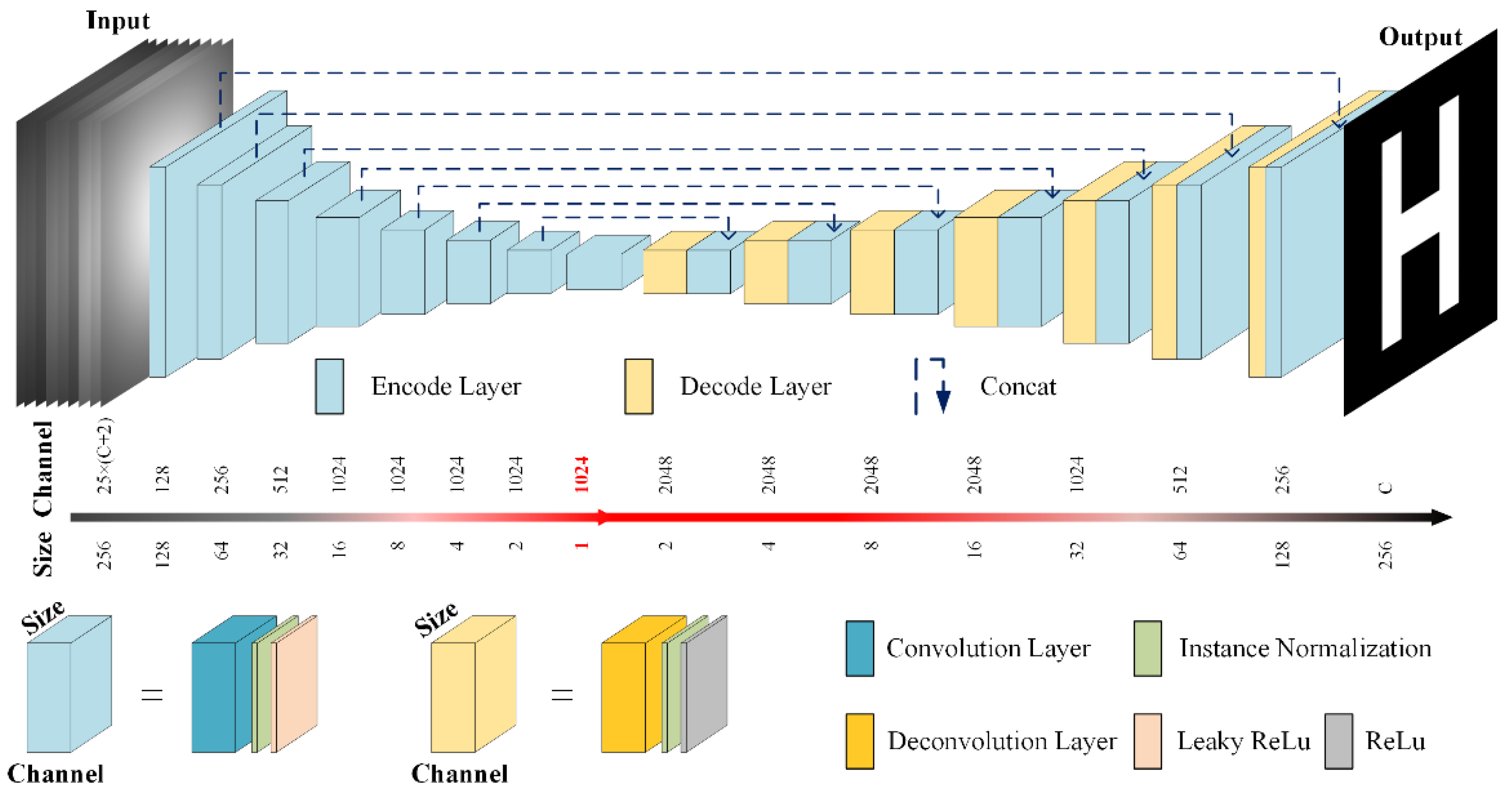
The deep learning model employed herein adopts the UNET framework as the baseline, which has a symmetrical structure, including 8 encoding layers and 8 decoding layers. The network input is a stack of projected images as the laser scans different locations, and the output is the predicted hidden target image, as shown in Figure 2. To correlate the laser scanning position and the corresponding projected image, the scanning position coordinates are concatenated to the corresponding projected image. Each encoding layer consists of a convolution layer, an instance normalization layer, and a leaky rectified linear unit (Leaky ReLU) nonlinear activation function. The kernel size of the convolution layer is 4 × 4 and the stride is 2, which enables feature extraction and downsampling of the input image while doubling the number of output feature channels. The instance normalization layer accelerates the model convergence and keeps each image instance independent. The encoding layers encode and compress the input image and extract image features. Each decoding layer consists of a transposed convolutional layer, an instance normalization layer, and a ReLU nonlinear activation function. The kernel size of the transposed convolution layer is 4 × 4 and the stride is 2, thereby upsampling the input feature map and halving the number of feature channels. The last transposed convolutional layer outputs the restored hidden object image. The decoding layer enlarges the compressed features to the original input image size, which is equivalent to completing the decoding operation of the image. Same sized encoding and decoding layers are concatenated to combine shallow low-level features from the encoding layer and deep high-level features from the decoding layer, which enables the back-propagation signal to be directly passed to the bottom layer, solving the vanishing gradient problem.
The loss function is used to calculate the difference between the prediction, f ^ and the ground truth, f, and the weights of the model are updated according to the loss function. The loss function of the reconstructed model includes a multiscale L2 loss function and structural similarity (SSIM), defined as follows:
M S E = 1 M × N × C k = 1 C i = 1 M j = 1 N ( f ( i , j , k ) f ^ ( i , j , k ) ) 2
S S I M ( x , y ) = ( 2 μ x μ y + C 1 ) ( 2 σ x y + C 2 ) ( μ x 2 + μ y 2 + C 1 ) ( σ x 2 + σ y 2 + C 2 )
L o s s = k γ k M S E k + α k β k ( 1 S S I M k ( f ^ , f ) )
where the resolution and channel of the image are M × N and C, respectively. μx and μy are the mean of x and y, respectively. σx and σy are the standard deviation of x and y, respectively. σxy is the covariance of x and y. C1 and C2 are constants related to the range of the image pixel values. k corresponds to different scales, and an additional transposed convolutional layer is used for the k-scale feature map to predict the image. γk is the weight of the mean square error (MSE) corresponding to the k-scale layer, and βk is the weight of the SSIM corresponding to the k-scale layer. α is a balance factor, indicating the trade-off of the loss function for MSE and SSIM. The MSE represents the noise average energy, which is the average energy of the error between the prediction, f ^ , and the ground truth, f. The closer the MSE is to 0, the higher the reconstruction accuracy. Since the MSE calculates the error between the pixels of the predicted image, f ^ , and the real image, f, it is more sensitive to the position of the target pixel in the predicted image. However, the correlation between pixels is ignored in the point-by-point calculation, making the MSE less sensitive to the structural information of the image. SSIM, on the other hand, evaluates the similarity between the prediction, f ^ , and the ground truth, f, in terms of the brightness, contrast, and structure. The SSIM values are in the [–1, 1] range, and a higher reconstruction accuracy is achieved if the values are closer to 1. The SSIM pays more attention to the structural information of the image, which is closer to the human subjective perception than the MSE. In general, the SSIM is insensitive to small translations and rotations in the reconstruction. The loss function consists of the MSE and SSIM, and it evaluates the accuracy of the predicted image from the reconstruction on both the structure and location metrics. The magnitudes of γk and βk increase closer to the output layer, which indicates that the predicted image has a greater impact on the loss function closer to the output layer.
The model training was performed on a 10th generation i9 server with a graphics processing unit (NVIDIA GeForce GTX 1080Ti) to accelerate the training. The training process was performed on the TensorFlow framework with Python 3.6. When training the model, the last three decoding layers were selected in the loss function to predict real images. γk and βk were set to 0.6, 0.8, and 1.0; α was set to 0.05. The batch size was set to 4. The initial value of the learning rate was set to 5 × 10⁻⁵, and the learning rate decay was adopted. The learning rate of each epoch was set to 5 × 10 5 1 . 0 + epoch / 3 . The adaptive moment estimation (ADAM) optimizer was used to iteratively update the weights of the model.

3. Results and Discussion

3.1. Simulation Results

The hidden target image, f, is transformed by the forward operator, A(l), to generate the projected image. The light transmission matrix A(l) is related to factors such as the laser intensity and the geometric parameters of the NLOS scene. A detailed discussion of the factors influencing A(l) is presented in the Supplementary Materials Section S2. The scene settings for discussing the impact factors of A(l) are shown in Figure S1, whereas the effect of the factors on the ill-conditioned degree of the light transmission matrix A(l) is shown in Figures S2 and S3. The light transmission matrix indicates that each pixel of the hidden object will contribute to all projection pixels, and a column of A(l) represents the physical impulse response of one pixel of the object. In the current scenario, the aim of deep learning was to learn the mapping between projections and the hidden target, i.e., inverse light transport process. In order to prove that the method is capable of learning this mapping, we designed a simulation consisting of randomly superimposed target units.

3.1.1. Projected Image Simulation

The setup of the NLOS scene is shown in Figure 3a. When the laser scans different positions on the wall, different light fields are generated. Under different light fields, several projection intensity images are formed on the wall due to the target. The projection intensity image of the target can be simulated corresponding to a laser scanning position based on Equation (6). As shown in Figure 3b, the laser sequentially scans a 5 × 5 array of positions on the wall. An image of the target “H” is shown in Figure 3c, and the projection intensity images corresponding to 25 laser scanning positions are shown in Figure 3d. Noise was added to the simulated projections in order to show the influence of interference, and the average SNR of the projected image after adding noise was 15.76 dB.
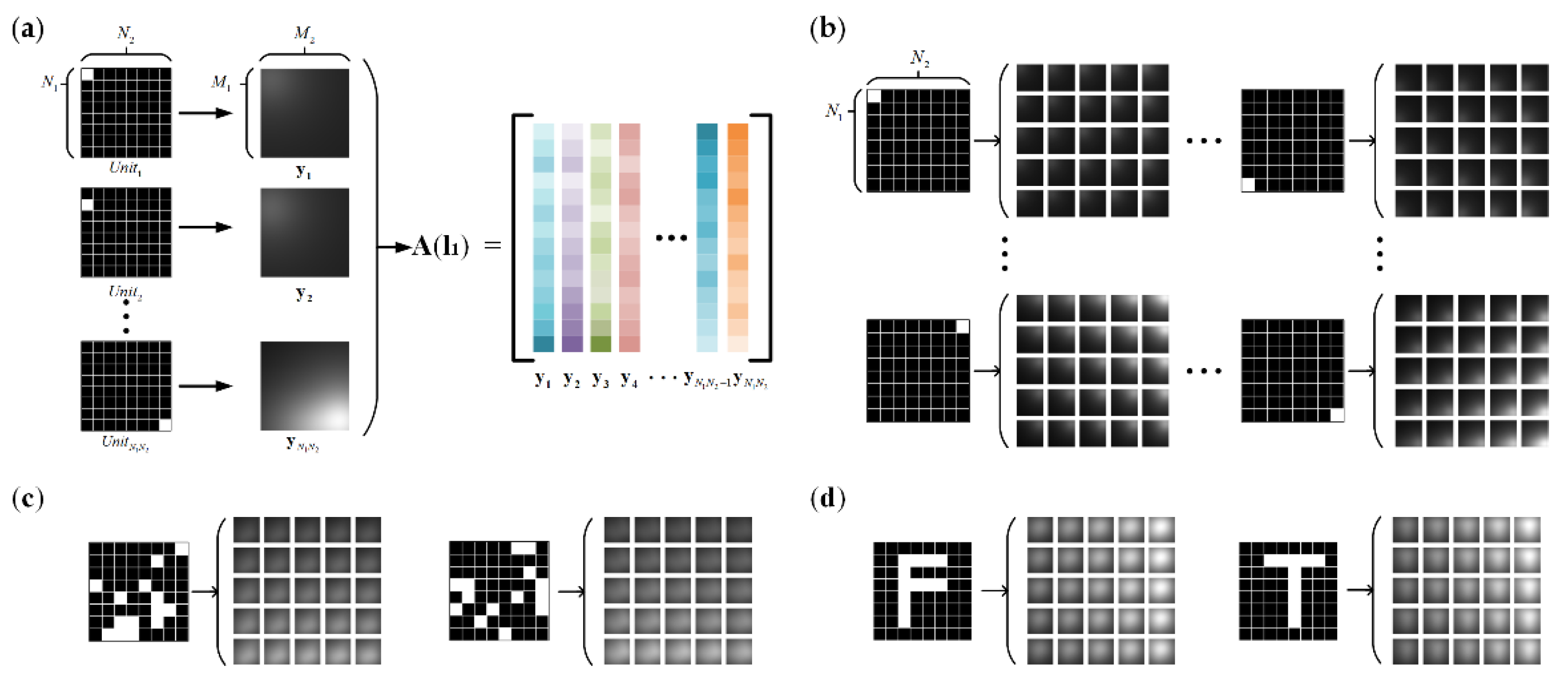
The hidden target area was divided into N1 × N2 units, where N1 = N2 = 8, and the intensity of each unit of the target was equal. When the laser scans the first position l1, which corresponds to position 1 in the 5 × 5 laser scanning array on the intermediate surface, the units of the hidden target generate projection intensity images in this light field with a resolution of M1 × M2, where M1 = M2 = 256. The projected intensity image is the physical response to the hidden target unit. When projected into a vector, this is equivalent to a column in the light transmission matrix A(l1). As shown in Figure 4a, the light transmission matrix A(l1) in the current light field was formed by the response of illuminating each unit of the hidden target. The laser sequentially scanned 25 positions on the intermediate surface, and each unit generated a corresponding set of 25 projected images. As shown in Figure 4b, all of the projected images of all of the units contained the complete information of 25 light transmission matrices in the different light fields. A hidden target can be obtained by superimposing the various target units. The projected image of the target is a weighted sum of the responses of these units, where the weights are based on the pixel intensities. Herein, the pixel intensities of the target units were equal, and theoretically, superimposing the target units can generate, at most, 2 N 1 × N 2 different targets. A total of 64 × 25 = 1600 projected images of 64 units were simulated, and 104 different hidden targets were generated from their projection samples by randomly superimposing 5~20 units. Figure 4c shows two examples of objects generated by randomly superimposing units. For the deep learning models, 400 samples were assigned to a test dataset and the remaining 9600 samples were divided 4:1 into a training dataset and a validation dataset. In addition to the 400 randomly superimposed test samples, a few meaningful test samples were generated by manually illuminating some units, such as the letter “F” and the letter “T”, as shown in Figure 4d.

3.1.2. Target Reconstruction with Simulated Data

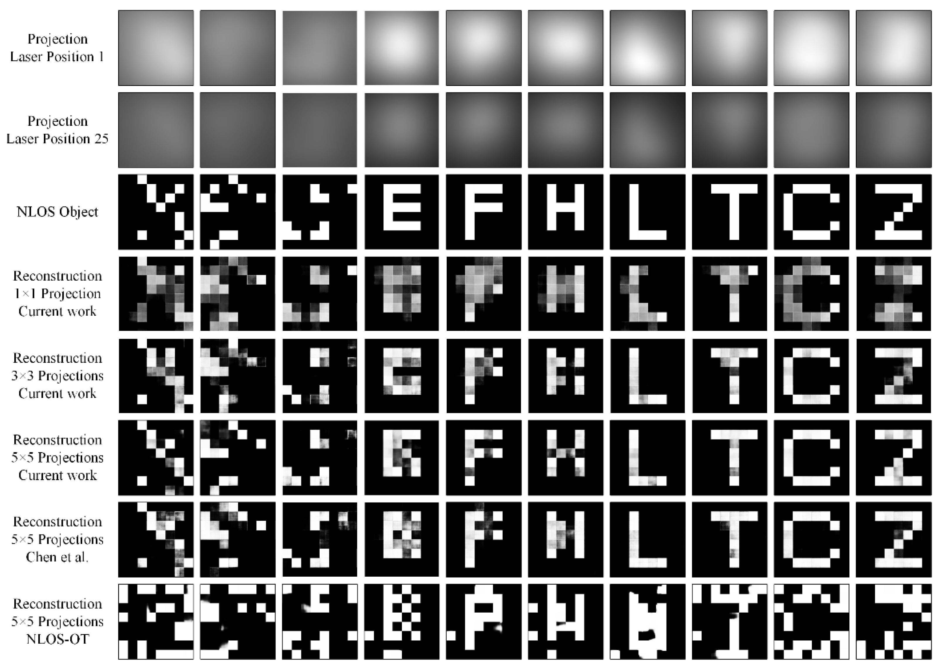
The projected images of the different light fields of the samples were stacked and then input for training into a deep learning model, and the reconstruction results of the tests are shown in Figure 5. The 3rd row of Figure 5 represents the hidden targets, where the first three test samples were selected from the test dataset, and the remaining seven test samples were designed such that they were meaningful targets. Scanning 25 positions generated 25 projected images. The 1st row and the 2nd row of Figure 5 show examples of the simulated projections corresponding to the laser scanning at positions 1 and 25, respectively. The input projected images and the output target had almost no common geometric features, which indicates that the hidden object cannot be directly identified from the projected images. For comparison purposes, reconstructions were performed using Chen’s method and the NLOS-OT framework, as shown in the 7th and 8th row of Figure 5, respectively, whereas the reconstructions obtained using our method are shown in the 6th row of Figure 5. The method of Chen et al. and our method used UNET as the baseline, where the architecture effectively suppresses image noise at the input and extracts features from the projected images. Although the reconstruction results were close to the ground truth, similar contributions from the adjacent target units to the projection can be observed due to the fact of isotropic diffuse reflections. Specifically, the mapping process can generate erroneous reconstructions, such as a missing target unit or artifacts adjacent to the target unit. As compared to the method of Chen et al., our method demonstrated fewer artifacts in the reconstruction. This is because a structural similarity indicator was introduced into the iterative model, which corrects the brightness, contrast, and structural information of the output of the network model. The NLOS-OT framework consists of an autoencoder (AE) and an encoder, which can be used for intensity-based NLOS imaging. Firstly, an autoencoder for manifold embedding was trained with the target image as the input and output to obtain the latent code of the target image. Secondly, another encoder for optimal transport mapped the projected images to the latent code of the target image. NLOS-OT had a tendency to learn the inverse light transport process when the dataset was widely distributed. Although a high reconstruction quality was obtained in the first step of the training, it was challenging to map the projections to the latent code of the targets in the second step. As a result, NLOS-OT was shown to produce more reconstruction errors than the other two methods.
The 4th row and the 5th row of Figure 5 show the reconstruction results of inputting stacking 1 × 1 projected images and stacking 3 × 3 projected images, respectively. The 3 × 3 projected images correspond to the laser positions 1, 3, 5, 11, 13, 15, 21, 23, and 25 in Figure 3b, whereas the 1 × 1 projected image corresponds to laser position 13. It is clear that fewer input projected images were prone to missing the target units and producing artifacts, thereby resulting in a poor reconstruction quality of the NLOS target. The input projected images contain the reflectance information of the target under varying light fields. For deep learning models to effectively learn the variations to reconstruct hidden object, dense scanning of the intermediate surface is necessary. This ensures that more projected images are obtained leading to a higher quality reconstruction. Our model performed well not only on the test dataset of randomly superimposed targets but also on the meaningful seven samples manually designed, thus validating that the method effectively learns the mapping between projections and the hidden object. A comparison of the reconstruction results from other numerical methods, such as the Jason-Van Cittert algorithm (JVC) [36], regularized least squares (RLS) [37], singular value decomposition (SVD) [38], and FISTA [39], is shown in Figure S4 in the Supplementary Materials Section S3.
The SSIM and peak signal-to-noise ratio (PSNR) are used to evaluate the quality of the reconstruction results of the simulated data, where larger SSIM and PSNR values indicate a higher reconstruction quality. Table 1 lists the SSIM and PSNR values for the test data using the NLOS-OT, the method of Chen et al., and our method using 25 projected images to reconstruct the target. Compared with the results of the other two methods, our method achieved a higher average SSIM and average PSNR, indicating a higher quality reconstruction of the NLOS target reconstructed by our model. From Table 1, it can also be seen that the rebuild rates of Chen’s and our methods were above 14 frames per second (FPS), and the difference was only 0.14%, with the reconstruction rate of Chen et al.’s method being marginally faster.

3.2. Experimental Results

3.2.1. Experimental Setup

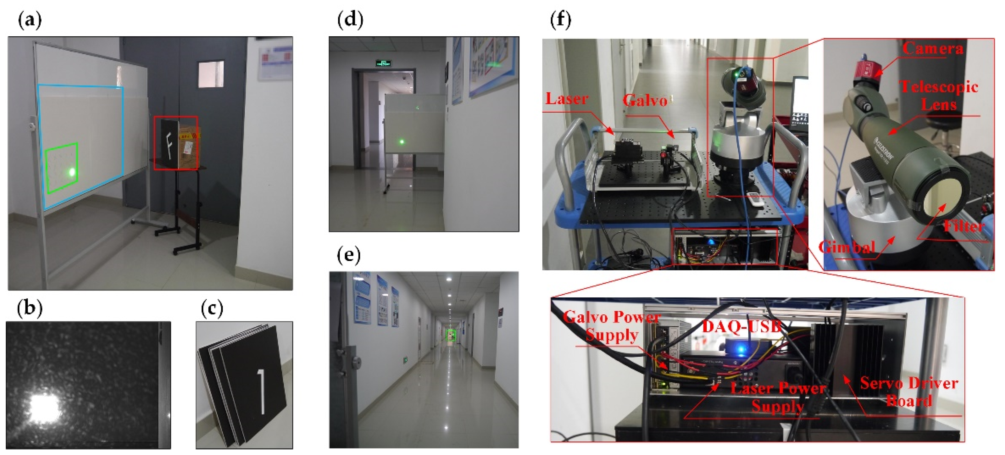
The setup for the NLOS scene is shown in Figure 6a, where the intermediate surface and a target were positioned at the corner of a corridor. Foam boards were used for the intermediate surface and target to facilitate diffuse reflections. In Figure 6a, the area selected by the blue box is the FOV of the camera, the area selected by the green box is the laser scanning region, and the area selected by the red box is the position of the NLOS target. A typical image captured by the camera is shown in Figure 6b, and the target sample is shown in Figure 6c. The target was obscured by the wall, and the camera could only capture the intensity information from the intermediate surface, as shown in Figure 6d. The experimental equipment was located at the other end of the corridor, and the distance between the equipment and the NLOS scene was 53.9 m. The area selected by the green box in Figure 6e is the location of the equipment. The layout of the experimental equipment is shown in Figure 6f. A current of 0.6 A was supplied to the laser, which was incident on the laser scanning area of the intermediate surface. The horizontal and vertical positions of the laser spot were controlled by the dual-axis galvanometer. The servo driver boards of the dual-axis galvanometer were powered by dual channel voltage outputs from the DAQ-USB. The pitch and yaw angles of the gimbal were adjusted such that the camera FOV was aimed at the intermediate surface. A narrow-band filter with transmission in the green spectrum was installed in front of the lens in order to reduce the interference from ambient light. The laser scanned a position, and the camera captured a corresponding projected image. The exposure time of the camera was set to 1000 ms, the gain was set to 10, the binning coefficients in the horizontal and vertical directions were set to 2, and the original image resolution was 1200 × 1920. With this configuration, scanning a 5 × 5 array of positions took approximately 25 s. Additional details of the NLOS scene setup can be found in Figure S5 and Tables S1–S3 in the Supplementary Materials Section S4.
Chen et al. simulated a dataset for training using the OpenGL rendering pipeline and then experimentally collected some samples for testing. We used their method to experiment at close range (~1 m) and long range (~50 m), as shown in Figures S6 and S7 in the Supplementary Materials Section S5. The results show that the model trained with a simulated dataset was only effective in an ideal environment under constraints of close range and low disturbance. In a close-range experiment, the laser diffraction was not appreciable, and the laser spot on the wall could be approximated as a point light source. However, for long distances, the laser diffraction could not be ignored, and it affected the projections generated by multiple reflections. Additionally, there were more environmental disturbances in the long range experiments, which resulted in a poor performance of the simulated dataset.
Due to the weak signal of the self-illuminous target unit, described in Section 3.1.1, the SNR of the captured projections was too low. Therefore, in the experiment, we did not use units as targets. Instead, the targets contained 10 numbers (0~9) and 8 letters (“A”, “H”, “V”, “X”, “F”, “L”, “K”, and “Z”). A total of 540 targets were generated after the data augmentation. A batch of long-distance data of hidden targets was collected under different light fields, which included 540 × 25 = 13,500 projected images, 25 images as a group, corresponding to 25 scanning positions on the intermediate surface. Eighteen objects and their projected images were chosen for the test data, and the remaining five hundred and twenty-two objects and their projected images were divided 8:1 into a training dataset and a validation dataset.

3.2.2. Target Reconstruction with Captured Data

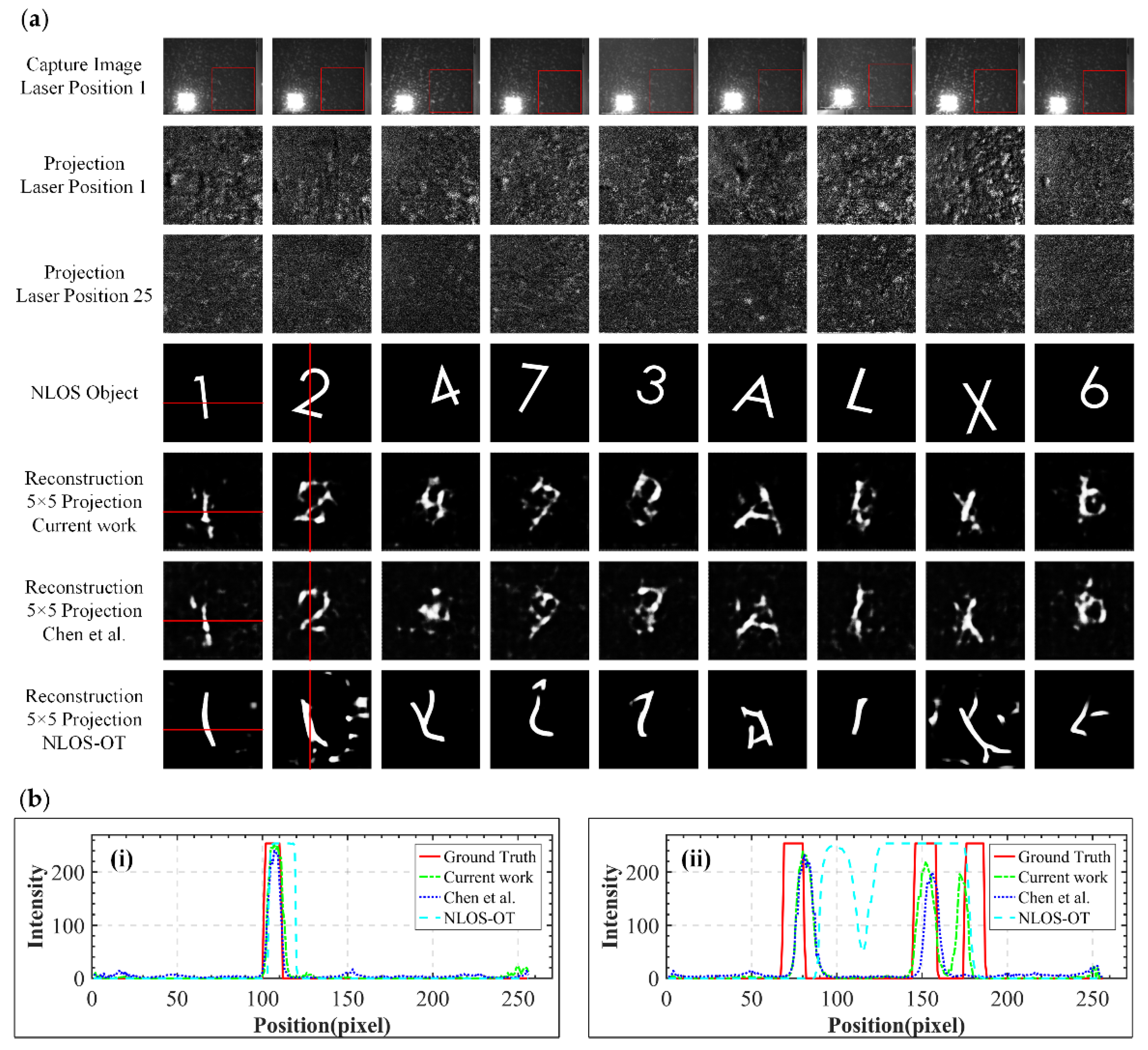
A typical image captured by the camera when the laser scanned the intermediate surface at position 1 is shown in the 1st row of Figure 7a, and the area selected by the red box is the selected ROI. The image captured by the camera shows that the laser diffraction was significant and strongly affected the already weak projection generated by the multiple diffuse reflections. Hence, background subtraction was performed to reduce the effects of the laser diffraction and other disturbances. The background subtraction was conducted by first removing the hidden objects and acquiring a set of background projected images, which were then subtracted from all acquired projected images of the hidden objects. The laser scanned 25 positions, and the corresponding projected images were captured by the camera. The 2nd row and the 3rd row of Figure 7a show examples of the background-subtracted projected images when the laser scanned the 1st and the 25th positions, respectively. The 4th row of Figure 7a shows nine targets for testing, and the reconstruction results of the remaining nine test targets are shown in Figure S8 in the Supplementary Materials Section S6. For comparison purposes, reconstructions were performed using the method of Chen et al. and the NLOS-OT, and the reconstruction results are shown in the 6th and 7th row of Figure 7a, respectively. The corresponding reconstruction results using our method are shown in the 5th row of Figure 7a. For all methods, 25 projected images were used as input to the models. Although the projected images were still disturbed by laser diffraction after the background subtraction, the UNET architecture was able to effectively learn the features of the projected images due to the fact of its noise suppression feature. In contrast, due to the hard trade-off between the manifold embedding accuracy and optimal transport accuracy, along with the difficulty of obtaining a strong generalization using a small-scale dataset, the NLOS-OT framework produced sharp but meaningless reconstructions.
As shown in Figure 7b, image (i) and image (ii) represent the pixel intensity along the red line in the digital “1” and “2” images, respectively. In image (i), the ground truth intensity was close to 255 at pixel positions 100~110, and the intensity at the other pixel positions was close to 0. In image (ii), the ground truth intensity was close to 255 at pixel positions 68~81, 145~159, and 175~187, and the intensity of the other pixel positions was close to 0. The reconstruction results show that our method had more accurate pixel intensity peaks and peak numbers than the reconstructed results of Chen et al. and the NLOS-OT. This was because our method obtained more accurate target information by correcting the image structure and suppressing the generation of artifacts. Additionally, our reconstruction results were more aligned with human subjective perception, which focuses on the structural information of predicted images. Finally, due to the artifact suppression effect of our model, weak structures in the reconstruction results were judged as artifacts and eliminated by the model.
SSIM and PSNR were used to evaluate the quality of the reconstruction results of the collected data. The reconstruction quality evaluated with 18 test targets is listed in Table 2. Compared with the results of the other two methods, our method achieved good performance on both the average SSIM and average PSNR. Our method achieved a higher average SSIM and average PSNR than Chen et al.’s, indicating a higher reconstruction quality of the NLOS target by our model. The rebuild rate of Chen et al.’s and our methods was above 14 FPS and differed only by 1.66%, with the method of Chen et al. showing a marginally faster rate. Although the PSNR and the reconstruction rate of Chen et al.’s and our methods were similar, in the case of the SSIM, our method significantly outperformed Chen et al.’s. This is because Chen et al.’s method does not account for structural corrections to the output prediction image. Compared with the NLOS-OT, our method achieved a higher average PSNR and rebuild rate while achieving a marginally lower average SSIM. In contrast to the widely distributed dataset of randomly superimposed target units in the simulation, the experiment only used a small-scale dataset with a narrower distribution, which makes the NLOS-OT more inclined to learn data priors rather than effective physical transformations. Therefore, the reconstruction results of the NLOS-OT are sharp but not accurate. The SSIM was not only affected by the image structure but also by the brightness and contrast. The sharp reconstruction by the NLOS-OT, due to the more accurate contrast and brightness, led to a marginally higher SSIM than with our method. However, structural distortion caused the PSNR of the NLOS-OT to be lower than our method. Overall, our method achieved a higher fidelity than the other two methods.

4. Conclusions

In summary, a practical long-range NLOS imaging system for long-distance data acquisition was demonstrated. A deep-learning-based NLOS object imaging method capable of correcting image structure was proposed. Based on the projected image formulation model, it was deduced that projected images were generated from hidden objects which were transformed by a highly ill-posed forward operator. It is difficult for deep learning to learn the light transport process under a single light field, but it can learn the spatial variation of the projected images under multiple light fields to alleviate the ill-posed nature of the problem. Taking advantage of this feature, a batch of data was collected under different light fields from long-distance NLOS scenes for training a deep learning model. The model utilized structural similarity to correct the structure of the output to suppress artifacts. The simulation and experimental results showed that compared with the method of Chen et al. and the NLOS-OT, our method achieved a higher fidelity, and the reconstruction results were closer to human subjective perception. Our method can image NLOS targets at distances beyond 50 m at a reconstruction rate of 14 FPS. Additionally, compared with conventional NLOS imaging, the proposed method only requires ordinary digital cameras to capture data, which is cost effective and has application potential in many real-life scenarios.
However, the proposed method still has some limitations. Firstly, our experiment was carried out in a corridor with an ideal environment, whereas real-world scenarios would be more complex. We will further expand the experiments to more types and more complex scenarios in the future. Secondly, uniform planar objects and diffuse surfaces were used in this study, whereas the reflection characteristics of hidden targets and diffuse surfaces in real-world scenes are complicated due to the fact of uneven surface conditions, uneven materials, and other interferences. Our future research will extend to more complex reflection characteristics of hidden targets and diffuse surfaces. Thirdly, our method used an active light source to change the light field to achieve different light transport processes, which is easily exposed in surveillance and covert imaging applications. Considering that a moving NLOS target can also produce changes in the light transport processes, further research will explore the use of passive NLOS imaging, which utilizes variations of projections caused by the moving target to achieve a more practical NLOS imaging technology.

Supplementary Materials

The following supporting information can be downloaded at: https://www.mdpi.com/article/10.3390/photonics10010025/s1, Figure S1: scene settings for discussing the impact factors of the light transmission matrix; Figure S2: Effect of the geometric parameters on the ill-conditioned degree of the light transmission matrix; Figure S3: Effect of the materials of the object and diffuse surface on the ill-conditioned degree of the light transmission matrix; Figure S4: Reconstruction results on the simulated projection and simulated projection with added noise using JVC, RLS, SVD, and FISTA; Figure S5: Coordinate system of the NLOS scene setup; Figure S6: Close-range experiment results; Figure S7: Long-range experiment results; Figure S8: Comparison of the reconstruction results of the remaining test targets on the captured data; Table S1: Geometric parameters of the hidden target; Table S2: Geometric parameters of the camera FOV; Table S3: Geometric parameters of the laser scanning positions.

Author Contributions

Conceptualization, X.C. and S.Z.; methodology, X.C.; software, X.C.; validation, X.C., S.Z., T.C. and M.L.; formal analysis, X.C.; investigation, S.Z., T.C. and M.L.; resources, S.Z.; data curation, X.C., T.C. and M.L.; writing—original draft preparation, X.C.; writing—review and editing, S.Z.; visualization, X.C.; supervision, S.Z.; project administration, S.Z. All authors have read and agreed to the published version of the manuscript.

Funding

This research was funded by the Zhejiang Provincial National Science Foundation of China (No. LY19F050016).

Institutional Review Board Statement

Not applicable.

Informed Consent Statement

Not applicable.

Data Availability Statement

The data presented in this study are available upon request from the corresponding author.

Acknowledgments

We are grateful for Chen et al.’s open source codes for allowing us to learn.

Conflicts of Interest

The authors declare no conflict of interest.

References

  1. Velten, A.; Willwacher, T.; Gupta, O.; Veeraraghavan, A.; Bawendi, M.G.; Raskar, R. Recovering three-dimensional shape around a corner using ultrafast time-of-flight imaging. Nat. Commun. 2012, 3, 745. [Google Scholar] [CrossRef] [PubMed] [Green Version]
  2. Arellano, V.; Gutiérrez, D.; Jarabo, A. Fast back-projection for non-line of sight reconstruction. In Proceedings of the ACM SIGGRAPH 2017 Posters, Los Angeles, CA, USA, 30 July–3 August 2017. [Google Scholar]
  3. Chan, S.; Warburton, R.E.; Gariepy, G.; Leach, J.; Faccio, D. Non-line-of-sight tracking of people at long range. Opt. Express 2017, 25, 10109–10117. [Google Scholar] [CrossRef] [PubMed]
  4. Jin, C.; Xie, J.; Zhang, S.; Zhang, Z.J.; Yuan, Z. Reconstruction of multiple non-line-of-sight objects using back projection based on ellipsoid mode decomposition. Opt. Express 2018, 26, 20089. [Google Scholar] [CrossRef] [PubMed]
  5. Jin, C.; Xie, J.; Zhang, S.; Zhang, Z.J.; Yuan, Z. Richardson–Lucy deconvolution of time histograms for high-resolution non-line-of-sight imaging based on a back-projection method. Opt. Lett. 2018, 43, 5885. [Google Scholar] [CrossRef] [PubMed]
  6. Marco, L.M.; Fiona, K.; Eric, B.; Jonathan, J.; Talha, S.; Andreas, V. Error Backprojection Algorithms for Non-Line-of-Sight Imaging. IEEE Trans. Pattern Anal. Mach. Intell. 2019, 41, 1615–1626. [Google Scholar]
  7. O’Toole, M.; Lindell, D.B.; Wetzstein, G. Confocal non-line-of-sight imaging based on the light-cone transform. Nature 2018, 555, 338–341. [Google Scholar] [CrossRef]
  8. Heide, F.; O’Toole, M.; Zang, K.; Lindell, D.B.; Wetzstein, G. Non-line-of-sight Imaging with Partial Occluders and Surface Normals. ACM Trans. Graph. 2019, 38, 1–10. [Google Scholar] [CrossRef] [Green Version]
  9. Huang, L.; Wang, X.; Yuan, Y.; Gu, S.; Shen, Y. Improved algorithm of non-line-of-sight imaging based on the Bayesian statistics. JOSA A 2019, 36, 834–838. [Google Scholar] [CrossRef]
  10. Shi, Z.; Wang, X.; Li, Y.; Sun, Z.; Zhang, W. Edge re-projection method for high-quality edge reconstruction in non-line-of-sight imaging. Appl. Opt. 2020, 59, 1793–1800. [Google Scholar] [CrossRef]
  11. Young, S.I.; Lindell, D.B.; Girod, B.; Taubman, D.; Wetzstein, G. Non-Line-of-Sight Surface Reconstruction Using the Directional Light-Cone Transform. In Proceedings of the 2020 IEEE/CVF Conference on Computer Vision and Pattern Recognition (CVPR), Seattle, WA, USA, 13–19 June 2020; pp. 1404–1413. [Google Scholar]
  12. Wu, C.; Liu, J.; Huang, X.; Li, Z.P.; Pan, J.W. Non-line-of-sight imaging over 1.43 km. Proc. Natl. Acad. Sci. USA 2021, 118, e2024468118. [Google Scholar] [CrossRef]
  13. Tanaka, K.; Mukaigawa, Y.; Kadambi, A. Polarized Non-Line-of-Sight Imaging. In Proceedings of the 2020 IEEE/CVF Conference on Computer Vision and Pattern Recognition (CVPR), Seattle, WA, USA, 13–19 June 2020; pp. 2133–2142. [Google Scholar]
  14. Torralba, A.; Freeman, W.T. Accidental pinhole and pinspeck cameras: Revealing the scene outside the picture. In Proceedings of the 2012 IEEE/CVF Conference on Computer Vision and Pattern Recognition (CVPR), Providence, RI, USA, 16–21 June 2012. [Google Scholar]
  15. Bouman, K.L.; Ye, V.; Yedidia, A.B.; Durand, F.; Freeman, W.T. Turning Corners into Cameras: Principles and Methods. In Proceedings of the 2017 IEEE International Conference on Computer Vision (ICCV), Venice, Italy, 22–29 October 2017. [Google Scholar]
  16. Saunders, C.; Murray-Bruce, J.; Goyal, V.K. Computational periscopy with an ordinary digital camera. Nature 2019, 565, 472–475. [Google Scholar] [CrossRef] [PubMed]
  17. Seidel, S.W.; Ma, Y.; Murray-Bruce, J.; Saunders, C.; Goyal, V.K. Corner Occluder Computational Periscopy: Estimating a Hidden Scene from a Single Photograph. In Proceedings of the 2019 IEEE International Conference on Computational Photography (ICCP), Tokyo, Japan, 15–17 May 2019. [Google Scholar]
  18. Yedidia, A.B.; Baradad, M.; Thrampoulidis, C.; Freeman, W.T.; Wornell, G.W. Using unknown occluders to recover hidden scenes. In Proceedings of the 2019 IEEE/CVF Conference on Computer Vision and Pattern Recognition(CVPR), Long Beach, CA, USA, 15–20 June 2019; pp. 12231–12239. [Google Scholar]
  19. Saunders, C.; Bose, R.; Murray-Bruce, J.; Goyal, V.K. Multi-depth computational periscopy with an ordinary camera. In Proceedings of the ICASSP 2020—2020 IEEE International Conference on Acoustics, Speech and Signal Processing (ICASSP), Barcelona, Spain, 4–8 May 2020; pp. 9299–9305. [Google Scholar]
  20. Seidel, S.W.; Murray-Bruce, J.; Ma, Y.; Yu, C.; Goyal, V.K. Two-Dimensional Non-Line-of-Sight Scene Estimation from a Single Edge Occluder. IEEE Trans. Comput. Imaging 2021, 7, 58–72. [Google Scholar] [CrossRef]
  21. Caramazza, P.; Boccolini, A.; Buschek, D.; Hullin, M.; Higham, C.F.; Henderson, R.; Murray-Smith, R.; Faccio, D. Neural network identification of people hidden from view with a single-pixel, single-photon detector. Sci. Rep. 2018, 8, 11945. [Google Scholar] [CrossRef] [PubMed] [Green Version]
  22. Aittala, M.; Sharma, P.; Murmann, L.; Yedidia, A.B.; Wornell, G.W.; Freeman, W.T.; Durand, F. Computational mirrors: Blind inverse light transport by deep matrix factorization. arXiv 2019, arXiv:1912.02314. [Google Scholar]
  23. Chen, W.; Daneau, S.; Mannan, F.; Heide, F. Steady-state non-line-of-sight imaging. In Proceedings of the 2019 IEEE/CVF Conference on Computer Vision and Pattern Recognition (CVPR), Long Beach, CA, USA, 15–20 June 2019; pp. 6790–6799. [Google Scholar]
  24. Musarra, G.; Caramazza, P.; Turpin, A.; Lyons, A.; Higham, C.F.; Murray-Smith, R.; Faccio, D. Detection, identification, and tracking of objects hidden from view with neural networks. In Proceedings of the Advanced Photon Counting Techniques XIII, Baltimore, MD, USA, 17–18 April 2019; p. 1097803. [Google Scholar]
  25. Chen, W.; Wei, F.; Kutulakos, K.N.; Rusinkiewicz, S.; Heide, F. Learned feature embeddings for non-line-of-sight imaging and recognition. ACM Trans. Graph. (TOG) 2020, 39, 1–18. [Google Scholar] [CrossRef]
  26. Chopite, J.G.; Hullin, M.B.; Wand, M.; Iseringhausen, J. Deep non-line-of-sight reconstruction. In Proceedings of the 2020 IEEE/CVF Conference on Computer Vision and Pattern Recognition (CVPR), Seattle, WA, USA, 13–19 June 2020; pp. 960–969. [Google Scholar]
  27. Metzler, C.A.; Heide, F.; Rangarajan, P.; Balaji, M.M.; Viswanath, A.; Veeraraghavan, A.; Baraniuk, R.G. Deep-inverse correlography: Towards real-time high-resolution non-line-of-sight imaging. Optica 2020, 7, 63–71. [Google Scholar] [CrossRef]
  28. Zhou, C.; Wang, C.-Y.; Liu, Z. Non-line-of-sight imaging off a phong surface through deep learning. arXiv 2020, arXiv:2005.00007. [Google Scholar]
  29. Zhu, D.; Cai, W. Fast Non-line-of-sight Imaging with Two-step Deep Remapping. arXiv 2021, arXiv:2101.10492. [Google Scholar] [CrossRef]
  30. Geng, R.; Hu, Y.; Lu, Z.; Yu, C.; Li, H.; Zhang, H.; Chen, Y. Passive Non-Line-of-Sight Imaging Using Optimal Transport. IEEE Trans. Image Process. 2022, 31, 110–124. [Google Scholar] [CrossRef]
  31. Jin, K.H.; McCann, M.T.; Froustey, E.; Unser, M. Deep convolutional neural network for inverse problems in imaging. IEEE Trans. Image Process. 2017, 26, 4509–4522. [Google Scholar] [CrossRef] [Green Version]
  32. Rick Chang, J.; Li, C.-L.; Poczos, B.; Vijaya Kumar, B.; Sankaranarayanan, A.C. One network to solve them all--solving linear inverse problems using deep projection models. In Proceedings of the IEEE International Conference on Computer Vision, Venice, Italy, 22–29 October 2017; pp. 5888–5897. [Google Scholar]
  33. Shah, V.; Hegde, C. Solving linear inverse problems using gan priors: An algorithm with provable guarantees. In Proceedings of the 2018 IEEE International Conference on Acoustics, Speech and Signal Processing (ICASSP), Calgary, AB, Canada, 15–20 April 2018; pp. 4609–4613. [Google Scholar]
  34. Wang, F.; Eljarrat, A.; Müller, J.; Henninen, T.R.; Erni, R.; Koch, C.T. Multi-resolution convolutional neural networks for inverse problems. Sci. Rep. 2020, 10, 5730. [Google Scholar] [CrossRef] [PubMed] [Green Version]
  35. Phong, B.T. Illumination for computer generated pictures. Commun. ACM 1975, 18, 311–317. [Google Scholar] [CrossRef] [Green Version]
  36. Akkoul, S.; Ledee, R.; Leconge, R.; Leger, C.; Harba, R.; Pesnel, S.; Lerondel, S.; Lepape, A.; Vilcahuaman, L. Comparison of image restoration methods for bioluminescence imaging. In Proceedings of the International Conference on Image and Signal Processing, Cherbourg-Octeville, France, 1–3 July 2008; pp. 163–172. [Google Scholar]
  37. Poggio, T.; Girosi, F. Networks for approximation and learning. Proc. IEEE 1990, 78, 1481–1497. [Google Scholar] [CrossRef]
  38. Van Loan, C.F. Generalizing the singular value decomposition. SIAM J. Numer. Anal. 1976, 13, 76–83. [Google Scholar] [CrossRef]
  39. Beck, A.; Teboulle, M. A Fast Iterative Shrinkage-Thresholding Algorithm for Linear Inverse Problems. Siam J. Imaging Sci. 2009, 2, 183–202. [Google Scholar] [CrossRef]
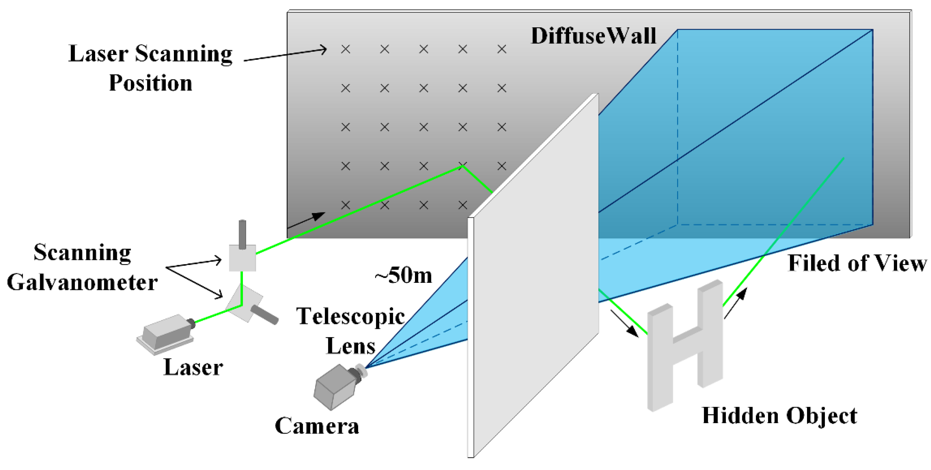
Figure 1. Non-line-of-sight (NLOS) imaging system setup.
Photonics 10 00025 g001
Figure 2. Detailed architecture of the reconstruction model.
Photonics 10 00025 g002
Figure 3. (a) NLOS scene; (b) laser scanning sequence; (c) hidden target example; (d) projected images corresponding to laser scanning positions.
Photonics 10 00025 g003
Figure 4. Simulated projections: (a) the hidden target unit and its projected image of the laser position l1; (b) the laser scanned a 5 × 5 array of the positions, and the corresponding projected images of the target units were generated on the intermediate surface; (c) two examples of randomly superimposed target units and their corresponding projected images; (d) two examples of meaningful test objects and their projected images.
Photonics 10 00025 g004
Figure 5. Comparison of the reconstruction results on the simulated data.
Photonics 10 00025 g005
Figure 6. Setup of the NLOS scene and experimental system: (a) NLOS scene setup; (b) camera field of view (FOV); (c) hidden object; (d) obstructed view; (e) experimental system setup position; (f) experimental system setup.
Photonics 10 00025 g006
Figure 7. (a) Comparison of the reconstruction results of the test targets on the captured data; (b) intensity plots from a line profile of the objects, where image (i) and image (ii) represent the pixel intensity along the red line in the digital “1” and “2” images, respectively.
Photonics 10 00025 g007
Table 1. Reconstruction quality comparison of methods on simulated data.
MethodSSIMPSNR (dB)Rebuild Rate (FPS)
NLOS-OT0.72517.298.14
Chen et al.0.880217.8914.18
Current work0.919318.7714.16
Table 2. Reconstruction quality comparison of the methods on the captured data.
MethodSSIMPSNR (dB)Rebuild Rate (FPS)
NLOS-OT0.864112.267.91
Chen et al.0.358313.7615.05
Current work0.815413.8114.80
Disclaimer/Publisher’s Note: The statements, opinions and data contained in all publications are solely those of the individual author(s) and contributor(s) and not of MDPI and/or the editor(s). MDPI and/or the editor(s) disclaim responsibility for any injury to people or property resulting from any ideas, methods, instructions or products referred to in the content.