Abstract
Progress in the field of machine learning has enhanced the development of self-adjusting optical systems capable of autonomously adapting to changing environmental conditions. This study demonstrates the concept of self-adjusting optical systems and presents a new approach based on reinforcement learning methods. We integrated reinforcement learning algorithms into the setup for tuning the laser radiation into the fiber, as well as into the complex for controlling the laser-plasma source. That reduced the dispersion of the generated X-ray signal by 2–3 times through automatic adjustment of the position of the rotating copper target and completely eliminated the linear trend arising from the ablation of the target surface. The adjustment of the system was performed based on feedback signals obtained from the spectrometer, and the movement of the target was achieved using a neural network-controlled stepper motor. As feedback, the second harmonic of femtosecond laser radiation was used, the intensity of which has a square root dependence on the X-ray yield. The developed machine learning methodology allows the considered systems to optimize their performance and adapt in real time, leading to increased efficiency, accuracy, and reliability.
1. Introduction
Nowadays, neural networks are finding increasing applications in optics and photonics. In the earlier works of machine learning, genetic algorithms were primarily used for pattern recognition, image reconstruction, aberration correction, or optical component design [1]. Subsequent studies focused on the analysis of large datasets [2] and inverse problems, where the superior ability of machine learning to classify data, uncover hidden structures, and handle a large number of degrees of freedom led to significant breakthroughs [3]. Neural networks have achieved great success in the design of nanomaterials [4], cell classification [5], super-resolution microscopy [6], quantum optics [7], and optical communications [8]. In addition to their application in general data processing, machine learning methods have the potential to control ultrafast photonics technologies of the next generation. This is due to the growing demand for adaptive control and self-adjustment of laser systems, as well as the fact that many ultrafast phenomena in photonics are nonlinear and multidimensional, with dynamics highly sensitive to noise [3]. Although advances in measurement techniques have led to significant developments in experimental methods, recent research has shown that machine learning algorithms provide new ways to identify coherent structures in large sets of noisy data and potentially determine fundamental physical models and equations based on the analysis of complex time series [3]. Neural networks can also greatly facilitate and automate the alignment process of complex optical systems such as femtosecond oscillators [9]. Machine learning with reinforcement has recently been used for this purpose. For example, it has been used for mode synchronization in femtosecond and picosecond oscillators [9,10], seed generation for free-electron lasers [11], soliton and chaos control in laser systems [12,13], and laser processing of silicon [14]. In any case, machine learning provides the opportunity to automate the adjustment of complex systems under changing external conditions. This has made this approach attractive for optimizing (increasing stability and signal level) the created laser-plasma source. The physics of X-ray generation in a laser-plasma source can be described as follows. When a laser pulse is focused on the surface of a solid target, the laser pulse energy is absorbed in the skin layer, generating laser-induced plasma with a temperature of several hundred electron volts and a solid density. During this short period, X-ray radiation is generated, as electrons cannot transfer a significant portion of their energy back to the lattice [15]. These fast electrons, arising from the interaction of the incident laser radiation with the plasma, lead to the generation of characteristic lines as the electron vacancy in the inner shell is filled from the outer shell [16]. To achieve a high X-ray flux, it is necessary to tightly focus the laser pulse, resulting in a focal spot size of a few micrometers, making the setup extremely sensitive to target position [15]. Therefore, target vibrations modulate the X-ray pulse. Additionally, due to the high intensity, surface ablation (removal of surface material) occurs, resulting in the reduction of the diameter of the rotating target over time, causing the focus to drift away from the target surface. As a result, the X-ray signal becomes unstable over time, and constant target-position adjustment is required due to target ablation.
Therefore, the main aim of this study was to develop an experimental setup based on reinforcement learning that would stabilize and maximize the amplitude of the X-ray signal generated in a laser-plasma source when ultrashort laser pulses are focused onto the surface of a rotating copper target. Additionally, the neural network created can be used for automatic control of the laser pulse propagation direction.
2. Materials and Methods
2.1. Experimental Setup
In the experiments, a femtosecond ytterbium fiber laser ANTAUS-10W-40u/250K (Avesta Project, Troitsk, Russia) with a wavelength of 1030 nm and an average power of up to 20 W was used. The pulse repetition rate was 2.0 MHz, with a maximum pulse energy of 10 µJ and a laser pulse duration of approximately 280 fs (M2 = 1.2). The laser radiation was focused (intensity on the target surface ~2.5 × 10¹⁴ W/cm2) onto the end of a rotating and vertically cyclically displaced copper cylinder (diameter 44 mm, thickness 8 mm) using a microscopic objective PAL-20-NIR-HR-LC00 with a focal length of 10 mm (NA ~0.3, spot diameter on the target ~4 µm). A target with a polished side surface (roughness of 0.5 µm or less) was mounted on a motor shaft taken from a hard disk. The vibrations of the rotating surface on the shaft did not exceed 2 µm (mean square root value over 10 min interval). This displacement algorithm allowed a single target to be operated for at least 5 h—during this time interval the dispersion of the X-ray intensity did not exceed 15%. To prevent deposition of ablated particles on the focusing optics, a compressed air blowing system was assembled in the exposure area. The ablated particles were carried away by the airflow through a thin tube and then sucked away by a vacuum cleaner.
X-ray radiation was measured using a single-channel scintillation detector SCSD-4 (Radikon, St. Petersburg, Russia) placed 13 cm away from the target. Attenuating copper or aluminum filters were installed in front of the detector for high radiation fluxes. The focus position relative to the target was controlled based on the intensity of the X-ray radiation. The second harmonic signal was focused into the HR USB4000 fiber spectrometer (Ocean Insight, Rochester, NY, USA).
The rotating target was mounted on a motorized 5-axis table. Control of the table movement was achieved using a WiFi2Duet stepper motor driver. The investigated samples were also placed on a three-axis motorized table and controlled by a similar driver. Signal collection was fully automated using LabVIEW, with simultaneous registration of X-ray signal intensity, source size (based on the second harmonic signal), second harmonic spectrum, and second harmonic signal intensity. The schematic diagram of the experimental setup is shown in Figure 1. The intensity of the second harmonic signal unambiguously determined the number of X-ray quanta generated during copper target ablation; thus, the spectral brightness at a wavelength of 515 nm was used as the feedback signal. A UDP server was used for data transmission to the neural network on the computer. HTTP protocol was used to control the neural network by the motion the stepper motors. In this configuration, a working speed of 10 Hz was achieved. The neural network controlled the stepper motor, moving the target along the optical axis. As a model experiment, the task of coupling laser radiation (at a wavelength of ~600 nm) into a fiber connected to a spectrometer was considered. For this purpose, a special node was developed, which was inserted into the kinematic alignment KM-100.
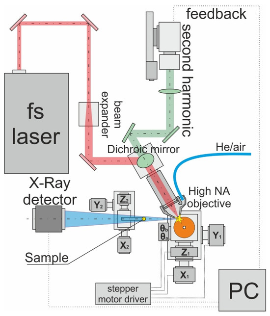
Figure 1.
Experimental setup. The laser pulse beam is tightly focused on the surface of the rotated Cu target, which leads to the generation of the X-ray. The sample is inserted inside the X-ray beam, and transmitted through the sample X-ray beam registered by the X-ray detector. In addition to the X-ray, the second harmonic (515 nm) is generated during laser–matter interaction. The second harmonic is collimated by the objective and transmitted to the spectrometer. The second harmonic is used as a feedback for the machine learning algorithm. Based on the signal, the Cu target location is changed by the motorized 5-axis stepper motor controlled by the driver.
2.2. Neural Network Architecture
The developed setup is based on the DQN learning algorithm [16]. Deep Q-Network (DQN) is a popular algorithm used in reinforcement learning, which combines the Q-learning algorithm with deep neural networks to train an agent with optimal action strategies in a given environment. The environment is the system or object (in our case, the current coordinates and feedback signal amplitude) that the agent interacts with, while the agent represents the reinforcement learning algorithm. The process starts with the environment sending its initial state (state = S) to the agent, who then takes an action (action = A—either movement or no action) based on its values in response to this state. The environment then sends the agent a new state (state′ = S′) and a reward (reward = K). The agent updates its knowledge based on the reward returned by the environment for the last action, and the cycle repeats. The cycle continues until the termination conditions of the learning process are met (either a specified number of actions are completed or the error level reaches a certain value). In DQN, the agent learns to choose actions based on the maximum expected future reward by using a neural network (NN) to approximate the Q-value function, which represents the expected reward for performing an action in a given state. The neural network takes the current state as input and outputs Q values for each possible action (see Figure 2). The Q function is computed using the following formula:
where γ is a number in the interval (0, 1), indicating the level of “greediness” of the algorithm. If γ approaches 0, the algorithm acts in a maximally “greedy” manner, seeking to maximize the next action. If γ approaches 1, the algorithm aims to maximize the overall gain on a larger scale. rt represents the reward at the current step. During the learning process, the agent interacts with the environment and stores its experience (i.e., state, action, reward, and next state) in a memory buffer. Initially, the agent acts randomly, with the probability of random actions exponentially decaying over time. The agent then selects a random mini-batch of the collected information from the buffer and uses it to update the Q-value function by minimizing the difference between the predicted Q values and the actual received rewards.
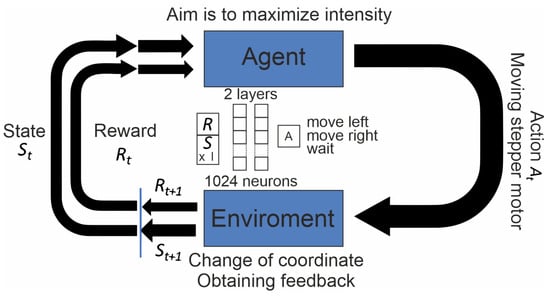
Figure 2.
Schematic representation of the algorithm. The agent receives information about environment (feedback and current coordinate) and reward. Based on the neural network (2 layers of 1024 neurons) it chooses one action: move left, move right or wait. The environment changes and the loop starts again.
The DQN (RL) algorithm was implemented based on two linear layers, each consisting of 1024 neurons. The training was performed on an Nvidia RTX 3070 (Nvidia, Santa-Clara, CA, USA) graphics card. The training parameters were set as follows: memory size of 100,000 elements, batch size of 1024 elements, learning rate of 10−4, Adam optimizer, MSE loss error criterion, and error decay rate of 5 × 10⁻⁴. In the NN, we used the current coordinate of the target (multiplied on the 0.001 factor) and the second harmonic intensity as feedback and) as inputs. These values were used as inputs for NN. The action (move left/move right/wait) is the output of the NN as it is presented in Figure 2.
The training parameters were selected after training the NN in the sandbox, as discussed further. The training was performed over 100,000 iterations, which guarantees a stable (close to 100%) result, i.e., the NN stabilizes the system in the verification stage (decreases dispersion and neutralizes the linear trend). During training, the NN initially acts randomly (for ~10,000 iterations, the possibility of the random action decays as 10−4), which is needed for filling the memory buffer. After that, the NN acts based on the result of developed algorithm. The learning process finishes when the error becomes smaller than 0.01 (if the number of iterations is higher than 20,000) or after 100,000 steps. The training procedure is completed in about two hours. In the working regime, it takes about one minute to achieve the optimal value.
Code is open-sourced and can be found at https://github.com/EvgMar/X_ray_AI.git (accessed on 28 September 2023).
2.3. Construction of the Reward Function
The key to the successful operation of the algorithm lies in the proper choice of rewards. In the case of an incorrectly defined reward function, the neural network will be unstable or learn too slowly. In the context of this setup, the neural network has three main actions to choose from: pause, move left, and move right. The objective is to move to the area with the maximum feedback signal and stay there for as long as possible. Therefore, the reward function was calculated as follows:
- −3 if the neural network suggests leaving the movement area (no movement occurs in this case).
- −1 × (It−1 − It) + (It − Imax)/Imax, where It is the signal amplitude at the current step, It−1 is the signal amplitude at the previous step, and Imax is the maximum amplitude over all previous steps, if the feedback amplitude decreases during the current step.
- (It−1 −It) + (It − Imax)/Imax, if the feedback amplitude increases during the current step.
- 0.5 if the pause occurs within the range of 0.9 Imax–Imax (due to fluctuations in the feedback signal).
- −(It − Imax)/Imax if the pause occurs within the range of 0.9 Imax–Imax (to avoid stopping outside the optimum).
By defining the reward function in this way, the error function does not grow exponentially (only at the boundaries, which is correct), and the neural network receives positive rewards in the area of maximum signal and during movement towards the maximum. This ensures high stability during operation.
3. Results and Discussion
3.1. Feedback Signal Selection
From a practical standpoint, the key parameters of a laser-plasma X-ray source are the X-ray flux, source size, stability of the X-ray signal, and ease of use. In order to address the ease of use, we have opted to operate the X-ray source without the need for a vacuum environment. Instead, X-rays are generated at the surface of a rotating copper cylinder, which continuously moves along the vertical axis. The laser pulse is tightly focused on the target surface, resulting in the formation of an electron plasma. During the duration of the laser pulse, a very short X-ray pulse is generated, as the laser-induced electrons are unable to transfer a significant portion of their energy back to the ions. This leads to the filling of vacancies in the inner shell from the outer shell, resulting in the generation of characteristic lines [16].
In our setup, the continuous movement of the target ensures that its time of usage is practically unlimited. However, two main issues arise. Firstly, the X-ray yield linearly decreases over time due to the ablation of the target surface by femtosecond laser pulses. Each pulse creates a small micromodification on the surface with an approximate depth of 1 µm. With a high repetition rate of approximately 2 MHz, the diameter of the target slowly decreases at a rate of about 1 µm every 10 min. As a result, the position of the laser focus shifts outward from the target surface, leading to a drop in X-ray yield and an increase in the size of the X-ray source. Additionally, the beats of the rotating target, with an amplitude of approximately 1 µm, introduce oscillations in the X-ray signal. It is also worth mentioning that the laser-induced plasma generates the second harmonic (SH) [17]. The intensity of the SH is determined by the parameters of the laser-induced plasma. Given that the X-ray yield also depends on the plasma electron density and temperature, we simultaneously measured the SH intensity and the X-ray yield, as shown in Figure 3.
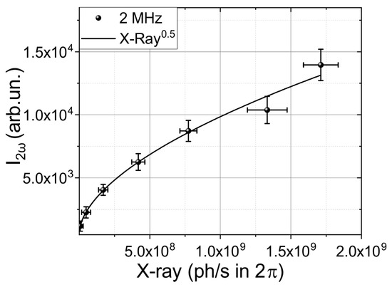
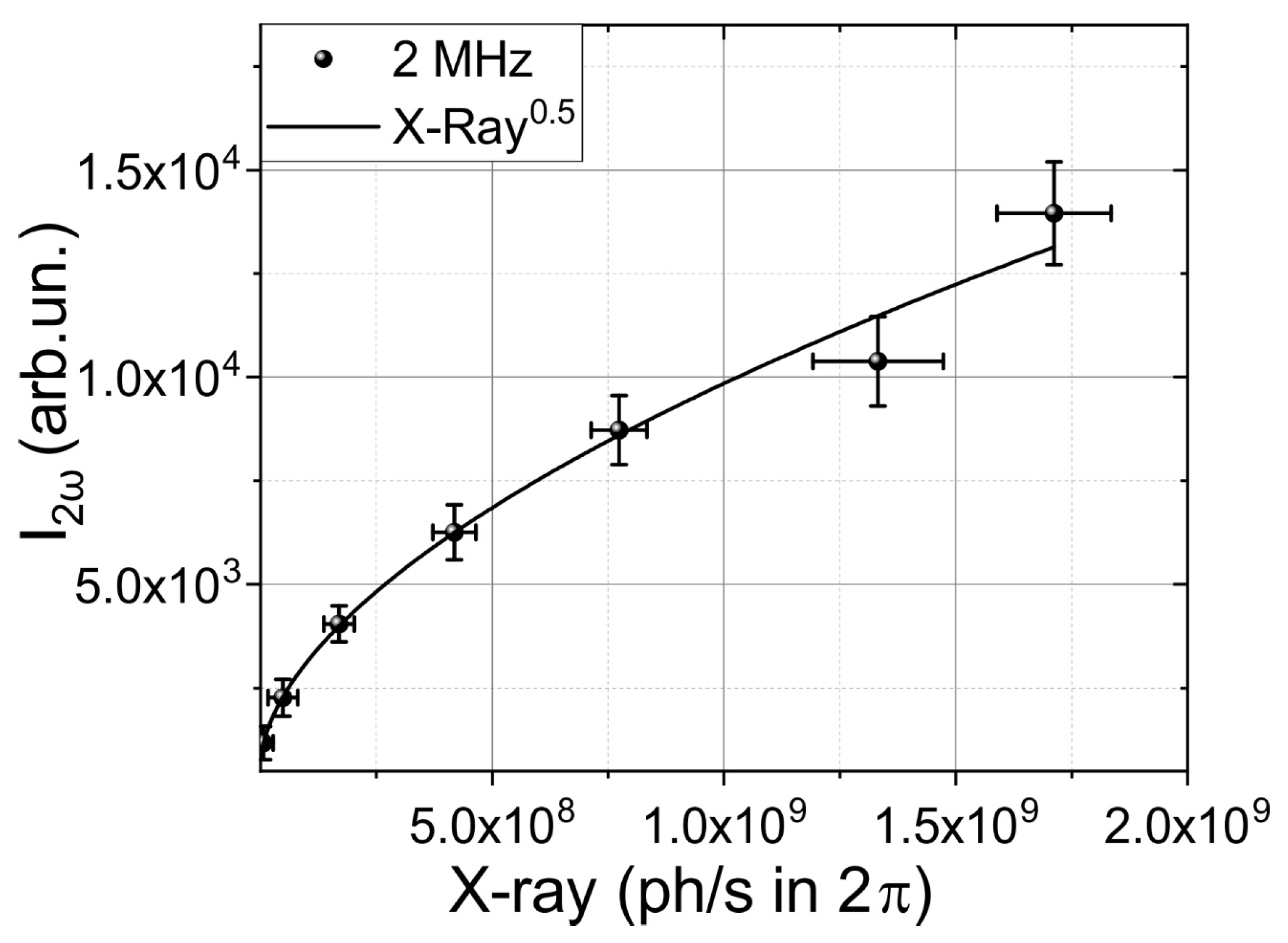
Figure 3.
Dependence of second harmonic intensity on X-ray photon flux at repetition frequencies of 2 MHz. The solid line shows square root dependence.
The square root dependence of the second harmonic (SH) on X-ray flux (see Figure 3) provides an opportunity to utilize the SH as feedback for reinforcement learning. The SH at a wavelength of 515 nm can be observed using various devices, such as CCD cameras, spectrometers, and photodetectors, including low-cost solutions. These devices offer different frequency ranges for measuring the SH intensity, ranging from MHz using photodetectors to kHz using cameras and approximately 100 Hz for spectrometers, providing a wide range of options. In our setup, we employed a scintillator detector with a frequency of 10 Hz, making the SH a particularly promising tool for incorporation into the feedback loop, due to the better possibilities for the scaling of working speed. However, during the validation process, we primarily focused on the X-ray signal as the key indicator, as end users are interested in a stable and high X-ray flux.
3.2. Checking the Operation and Stability of the Neural Network in the Sandbox
Initially, the neural network was tested without being connected to external sensors and control elements. This allowed the determination of initial values for the learning rate, the decay rate of the probability of random actions, and the coefficient γ. In this case, within the framework of the simulated environment, it was assumed that the signal intensity (feedback) was calculated as −1 × (x − x0)2, where x0 represents the initial position of the target. The neural network adjusted the coordinate x, while the target oscillated with a period T (100-time steps) and an amplitude A (10% of the maximum signal intensity). Additionally, the target moved linearly at a speed of 1/B (B = 5000), as shown in Figure 4.
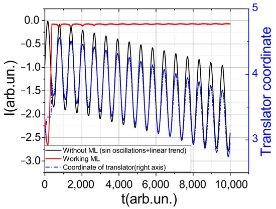
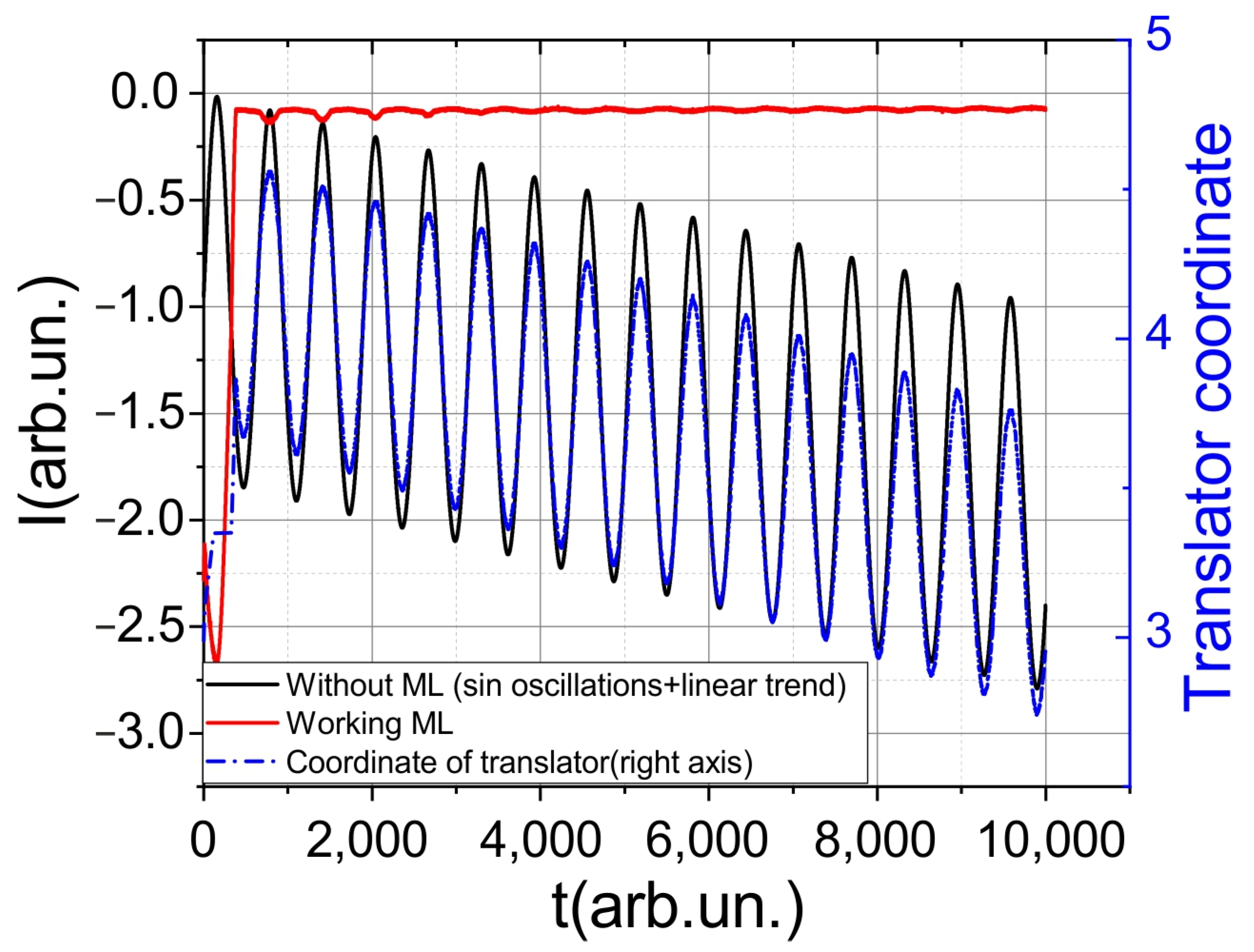
Figure 4.
Results of the neural network performance in a sandbox. The black line represents the signal variation without the work of the neural network, the red line represents the signal variation with the working neural network, and the blue line represents the change in coordinates.
The conducted performance evaluation demonstrated that the model maintains stability regardless of the initial positions. Furthermore, the model exhibits stability even when subjected to linear drift speeds up to four times higher than the training speeds. The range of stability is maintained when adjusting the frequency of oscillations within the range of f0/5 < f < 2f0, where f0 represents the oscillation frequency used during training. Through this testing in the simulated environment, initial parameters were identified for successful implementation in real experiments.
3.3. Coupling the Laser Pulse into a Fiber Using Reinforcement Machine Learning
The next modeling task involved coupling light into the fiber. For this purpose, the neural network was modified to perform movements in two coordinates, thereby adding two additional actions. The light was coupled inside the fiber, changing the angle of incidence of the laser beam onto the kinematic mirror mount (KM-100, Thorlabs, Newton, MA, USA). By adjusting two alignment screws, the angle of deviation of the laser beam could be changed, allowing for coupling into the spectrometer. In this setup, the maximum spectral brightness (signal intensity at a specific wavelength measured by the spectrometer) served as the feedback signal. Although the task may initially seem straightforward, the presence of play or backlash complicates the problem. When moving to the same coordinates on the controller, the laser beam may not return to the exact same point due to these mechanical imperfections.
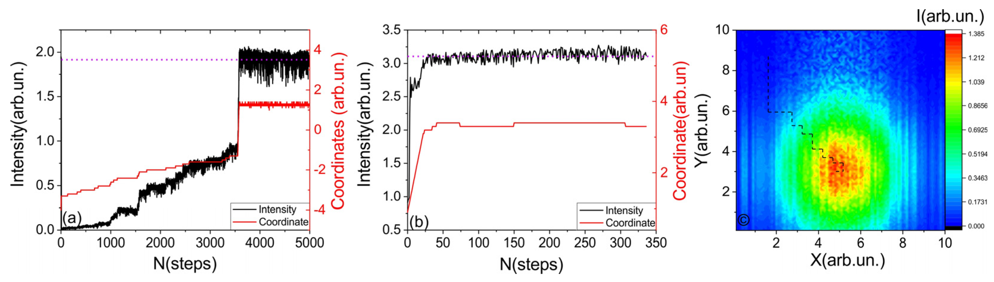
Figure 5 illustrates the results of the neural network’s operation in two different regimes. In the first case (Figure 5a), the maximum amplitude was not initially specified, while in the second case (Figure 5b), the maximum amplitude was specified. In the first case, the neural network determined the maximum value in the working process. As a result, the convergence to the operational regime was significantly slower in the first case. By plotting the trajectory of the laser beam coupling (see Figure 5c) on a two-dimensional intensity map (constructed by traversing all available coordinates), it can be observed that the coupling path with simultaneous movement along only one axis is close to optimal. However, the reverse movement along the x axis is affected by the presence of backlash in the system. It is worth noting that due to fluctuations in the signal of approximately 10%, the neural network exhibits small fluctuations along different axes in the vicinity of the maximum, without any significant changes in intensity.

Figure 5.
Working regime of neural network. The black line shows the intensity observed by spectrometer, red line shows stepper motor coordinate. (a) “Slow” regime, when no information about intensity level was given. (b) “Fast” regime, when the approximate maximum intensity was transmitted to the neural network. (c) The heat map of the intensity distribution for all x and y coordinates. The dashed line indicates the path that the network used to find optimal location pair (x,y).
From a practical perspective, several important aspects can be highlighted. The best convergence and stability of the neural network are achieved when the feedback signal is initially different from zero. Otherwise, significantly more training time (more than twice as much) is required, as the time spent searching for a non-zero signal level significantly affects the weights. Increasing the learning rate also has a negative impact on the stability of the neural network’s operation. The minimum required number of training iterations is on the order of 10,000. If fewer cycles of training are performed, the neural network does not learn, even if the training error suggests otherwise. This is probably due to insufficient exploration of the state space (coordinates, intensity) within the given time, resulting in the neural network encountering scenarios that were not adequately explored during training. From a practical standpoint, the most optimal trade-off between training time and stability is achieved with approximately 30,000 training steps. In such cases, it is possible to achieve successful fiber coupling from any starting position in nearly 100% of attempts (10 out of 10). Longer training times also contribute to stable operation.
3.4. Stabilising the Intencity of the X-ray Source
In the case of optimizing the laser-plasma source, the movement was performed along a single axis, and the second harmonic signal served as the feedback, which was detected using an Ocean Optics HR 4000 spectrometer. When optimizing X-ray pulse generation, the main objectives were compensating for target oscillations and addressing the linear drift caused by target ablation (where the laser pulse gradually removes part of the target surface at a rate of approximately 1 µm/minute). In some aspects, this task is even simpler, as achieving stable coupling to a single point is more challenging than compensating for periodic oscillations. This may be due to the fact that maintaining stability at a single point is not so robust as continuously compensating for oscillations. Figure 6 reveals the presence of a linear trend and complex beating signal, representing a superposition of multiple harmonic frequencies. The linear trend compensates for target drift, while the combined beating signal stabilizes the X-ray pulse.
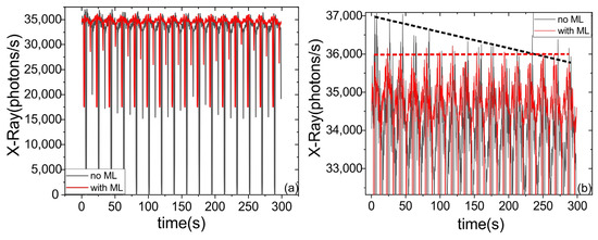
Figure 6.
Comparison of operating regimes of the laser-plasma source with and without the reinforcement learning-based automatic target position adjustment. (a) Dynamics of the X-ray signal variation in full scale. (b) Enlarged view of the graph in (a). The dotted lines show the linear trend due to laser ablation.
The conducted validation demonstrates several important features. Firstly, a significant reduction in X-ray signal oscillations by 2–3 times was achieved. Secondly, the linear trend that arose during the laser ablation of the target was effectively compensated, see Figure 6b. From the perspective of stability and robustness, similar parameters to the fiber coupling case were observed. Specifically, it is important to maintain a moderate learning rate (~10−4), and the initial feedback signal should be non-zero to ensure stability during the learning process. Furthermore, a training duration of more than 20,000 iterations is recommended to achieve a high level of stability and performance. The observed maxima in the initial stages of the X-ray yield was obtained on the small ledge that formed on the edge of the target where the stepper motor changed its direction (the ablation speed doubled during the turn). Due to local field enhancement on this edge, the X-ray yield increased. However, this led to the decrease in the mean signal. During the NN-based algorithm, the edge does not form and this maximum is less pronounced. It is also worth mentioning that the profile of the irradiated target is smother under ML control. Thereby, the use of the ML algorithm demonstrates the ability to compensate the complex vibrations and linear trends, and could also be used to compensate long-term temperature drift or low-frequency noise. We believe that such complex optical systems could in future be maintained by the AI-based algorithm, which would improve the stability of the system and will free up human resources for use in more creative tasks.
4. Conclusions
In conclusion, the optimization of laser-plasma X-ray sources using reinforcement learning techniques has shown promising results in improving stability and performance. Through the adjustment of the laser focus position, the X-ray signal output can be enhanced and stabilized. The incorporation of reinforcement learning algorithms allows adaptive optimization, compensating for target oscillations, linear drift, and other effects that may impact X-ray signal generation. The validation process demonstrated the effectiveness of reinforcement learning in reducing X-ray signal oscillations and compensating for linear trends during laser ablation. By carefully selecting learning parameters and ensuring a sufficient number of training iterations, stability and robustness can be achieved. Further research and experimentation in this field hold great potential for advancing the performance and reliability of laser-plasma X-ray sources, benefiting various applications such as material analysis, medical imaging, and industrial processes.
Author Contributions
Conceptualization, methodology, supervision, writing—original draft preparation and writing, E.M.; investigation, E.M., A.G., T.S., N.A. and V.R.; writing—review and editing all authors, funding acquisition, project administration, I.D. All authors have read and agreed to the published version of the manuscript.
Funding
This work was performed within the State assignment of Federal Scientific Research Center “Crystallography and Photonics” of the Russian Academy of Sciences (in part of “data processing”), under grant No. 075-15-2021-1362 (as part of “carrying out measurements on the laser microplasma X-ray source”).
Institutional Review Board Statement
Not applicable.
Informed Consent Statement
Not applicable.
Data Availability Statement
The code is open sourced and can be found at https://github.com/EvgMar/X_ray_AI.git (accessed on 28 September 2023). Data underlying the results presented in this paper are not publicly available at this time but may be obtained from the authors upon reasonable request.
Acknowledgments
E. Mareev thanks A. Ivchenko and Non-Commercial Foundation for the Advancement of Science and Education INTELLECT.
Conflicts of Interest
The authors declare no conflict of interest.
References
- Martin, S.; Rivory, J.; Schoenauer, M. Synthesis of Optical Multilayer Systems Using Genetic Algorithms. Appl. Opt. 1995, 34, 2247. [Google Scholar] [CrossRef]
- Zhou, J.; Huang, B.; Yan, Z.; Bünzli, J.C.G. Emerging Role of Machine Learning in Light-Matter Interaction. Light Sci. Appl. 2019, 8, 84. [Google Scholar] [CrossRef]
- Genty, G.; Salmela, L.; Dudley, J.M.; Brunner, D.; Kokhanovskiy, A.; Kobtsev, S.; Turitsyn, S.K. Machine Learning and Applications in Ultrafast Photonics. Nat. Photonics 2021, 15, 91–101. [Google Scholar] [CrossRef]
- Hegde, R.S. Deep Learning: A New Tool for Photonic Nanostructure Design. Nanoscale Adv. 2020, 2, 1007–1023. [Google Scholar] [CrossRef] [PubMed]
- Chen, C.L.; Mahjoubfar, A.; Tai, L.C.; Blaby, I.K.; Huang, A.; Niazi, K.R.; Jalali, B. Deep Learning in Label-Free Cell Classification. Sci. Rep. 2016, 6, 21471. [Google Scholar] [CrossRef] [PubMed]
- Durand, A.; Wiesner, T.; Gardner, M.A.; Robitaille, L.É.; Bilodeau, A.; Gagné, C.; De Koninck, P.; Lavoie-Cardinal, F. A Machine Learning Approach for Online Automated Optimization of Super-Resolution Optical Microscopy. Nat. Commun. 2018, 9, 5247. [Google Scholar] [CrossRef] [PubMed]
- Palmieri, A.M.; Kovlakov, E.; Bianchi, F.; Yudin, D.; Straupe, S.; Biamonte, J.D.; Kulik, S. Experimental Neural Network Enhanced Quantum Tomography. npj Quantum Inf. 2020, 6, 20. [Google Scholar] [CrossRef]
- Lugnan, A.; Katumba, A.; Laporte, F.; Freiberger, M.; Sackesyn, S.; Ma, C.; Gooskens, E.; Dambre, J.; Bienstman, P. Photonic Neuromorphic Information Processing and Reservoir Computing. APL Photonics 2020, 5, 020901. [Google Scholar] [CrossRef]
- Sun, C.; Kaiser, E.; Brunton, S.L.; Nathan Kutz, J. Deep Reinforcement Learning for Optical Systems: A Case Study of Mode-Locked Lasers. Mach. Learn. Sci. Technol. 2020, 1, 045013. [Google Scholar] [CrossRef]
- Yan, Q.; Deng, Q.; Zhang, J.; Zhu, Y.; Yin, K.; Li, T.; Wu, D.; Jiang, T. Low-Latency Deep-Reinforcement Learning Algorithm for Ultrafast Fiber Lasers. Photonics Res. 2021, 9, 1493. [Google Scholar] [CrossRef]
- Bruchon, N.; Fenu, G.; Gaio, G.; Lonza, M.; O’shea, F.H.; Pellegrino, F.A.; Salvato, E. Basic Reinforcement Learning Techniques to Control the Intensity of a Seeded Free-Electron Laser. Electronics 2020, 9, 781. [Google Scholar] [CrossRef]
- Kuprikov, E.; Kokhanovskiy, A.; Serebrennikov, K.; Turitsyn, S. Deep Reinforcement Learning for Self-Tuning Laser Source of Dissipative Solitons. Sci. Rep. 2022, 12, 7185. [Google Scholar] [CrossRef] [PubMed]
- Iwami, R.; Mihana, T.; Kanno, K.; Sunada, S.; Naruse, M.; Uchida, A. Controlling Chaotic Itinerancy in Laser Dynamics for Reinforcement Learning. Sci. Adv. 2022, 8, eabn8325. [Google Scholar] [CrossRef] [PubMed]
- Masinelli, G.; Le-Quang, T.; Zanoli, S.; Wasmer, K.; Shevchik, S.A. Adaptive Laser Welding Control: A Reinforcement Learning Approach. IEEE Access 2020, 8, 103803–103814. [Google Scholar] [CrossRef]
- Garmatina, A.A.; Asadchikov, V.E.; Buzmakov, A.V.; Dyachkova, I.G.; Dymshits, Y.M.; Baranov, A.I.; Myasnikov, D.V.; Minaev, N.V.; Gordienko, V.M. Microfocus Source of Characteristic X-rays for Phase-Contrast Imaging Based on a Femtosecond Fiber Laser. Crystallogr. Rep. 2022, 67, 1026–1033. [Google Scholar] [CrossRef]
- Rousse, A.; Audebert, P.; Geindre, J.P.; Falliès, F.; Gauthier, J.C.; Mysyrowicz, A.; Grillon, G.; Antonetti, A. Efficient K X-ray Source from Femtosecond Laser-Produced Plasmas. Phys. Rev. E 1994, 50, 2200–2207. [Google Scholar] [CrossRef]
- Garmatina, A.A.; Shubnyi, A.G.; Asadchikov, V.E.; Nuzdin, A.D.; Baranov, A.I.; Myasnikov, D.V.; Minaev, N.V.; Gordienko, V.M. X-ray Generation under Interaction of a Femtosecond Fiber Laser with a Target and a Prospective for Laser-Plasma X-ray Microscopy. J. Phys. Conf. Ser. 2021, 2036, 012037. [Google Scholar] [CrossRef]


Disclaimer/Publisher’s Note: The statements, opinions and data contained in all publications are solely those of the individual author(s) and contributor(s) and not of MDPI and/or the editor(s). MDPI and/or the editor(s) disclaim responsibility for any injury to people or property resulting from any ideas, methods, instructions or products referred to in the content. |
© 2023 by the authors. Licensee MDPI, Basel, Switzerland. This article is an open access article distributed under the terms and conditions of the Creative Commons Attribution (CC BY) license (https://creativecommons.org/licenses/by/4.0/).