Tensor-Train Decomposition-Based Hybrid Beamforming for Millimeter-Wave Massive Multiple-Input Multiple-Output/Free-Space Optics in Unmanned Aerial Vehicles with Reconfigurable Intelligent Surface Networks

Abstract

Unmanned aerial vehicles (UAVs) can support low-cost, highly mobile communications while making it possible to establish dedicated terrestrial networks. To overcome the pointing error (PE) and beam misalignment of millimeter-wave large-scale multiple-input multiple-output/free-space optics (MIMO/FSO) caused by UAV jitter, a millimeter-wave massive MIMO/FSO hybrid beamforming method based on tensor train decomposition is proposed. This approach is used for reconfigurable intelligent surface (RIS) network-assisted UAV millimeter-wave massive MIMO/FSO to improve system spectral efficiency. Firstly, the high-dimensional channel of RIS-assisted millimeter-wave massive MIMO/FSO in UAV is represented as a low-dimensional channel by tensor training decomposition. Secondly, the two-way gated recursive unit attention neural network model can effectively solve the FSO PE caused by UAV jitter, and the fast fading channel and Doppler frequency shift are estimated by the Fast Cyclic Tensor Power Method (FCTPM) based on tensor training decomposition. Finally, the RIS phase shift matrix is optimized by singular value decomposition. The hybrid beamforming and RIS phase-shift matrices were estimated by using the low-complexity phase extraction alternating minimization method to solve the beam misalignment problem. Simulation results show that by using the proposed method, the spectrum utilization rate is improved by 23.6% compared with other methods.

1. Introduction

In communication networks, ground base stations are vulnerable to destruction by natural disasters such as earthquakes, tsunamis and flash floods. As a result, the communication infrastructure in the disaster area is damaged, and communication services cannot be provided. This further hampers rescue operations. UAVs combined with cellular networks can support UAV communication at low cost and high mobility, and also provide the possibility of establishing new private ground networks [1,2,3]. In areas with dense urban traffic hotspots, the coverage of traditional cellular base stations cannot meet the demand. UAVs are highly flexible and easy to deploy. They can quickly provide coverage and service classification for hotspots, with a wide range of application scenarios. Air base stations (ABS) are more resilient to environmental changes than ground base stations [4]. Therefore, UAVs can also be deployed in areas without infrastructure coverage to provide emergency communication connections.

To improve the transmission performance of UAV communication, Relay-Assisted Free-Space Optical-Radio Frequency (RA-FSO-RF) was introduced into the communication system [5,6]. The Low Density Parity Coding Multiple-Input Multiple-Output/Free-Space Optical (LDPC-MIMO/FSO) method was used to evaluate the performance of Malaga distributed MIMO/FSO links with m-QAM and pointing error (PE) based on power series [7]. In the previous work, our team proposed a Dynamic Hybrid Precoding (DHP) double-hop hybrid FSO-RF system inspired by Manifold Learning (ML) based on antenna zoning algorithm [8]. MIMO technology can be used to eliminate the effects of atmospheric disturbance (AT) and pointing error (PE) on link performance in FSO systems [9]. Under the joint action of AT and PE, the bit error rate (BER) and channel capacity of MIMO systems using the optical space scheme are studied in the reference [10]. The communication environment of UAVs is greatly affected by AT. This is mainly because AT has a great influence on the performance of laser communication. The factors affecting the communication performance of UAVs mainly include visual axis error and jitter error. Scholars have studied the performance of hybrid free-space optical and radio frequency (FSO-RF) relay systems in the presence of AT and PE [11]. These studies on FSO-RF systems have addressed the issue of FSO link or trunk selection [12,13,14,15]. However, there have been few reports of PE and beam misalignment studies of millimeter-wave massive MIMO/FSO in UAV RF communication links.

The effective coverage of UAV base stations is affected by problems such as dynamic movement of UAVs and obstacles, beam shift and Doppler frequency shift caused by obstacle interference and wind speed [16,17]. Beamforming of UAV antenna arrays helps to overcome the problems of beam misalignment and Doppler shift to improve UAV communication performance. Beamforming designs can also be used for drone communication. The 3D location of UAV base stations with a certain number of indoor users and obstacles was determined [18]. UAV base stations can sense the location of users and obstacles for maximum coverage. A Zero Forcing Hybrid Beam Forming (ZF-HBF) method for downlink multi-user orthogonal frequency-division multiplexing systems is explored in [19,20,21]. This method was used to achieve beamforming according to the Spectral Efficiency (SE) of the system up to the maximum upper bound. In order to achieve fast beamforming training and tracking, the hierarchical structure of the beam codebook and the hierarchical codebook with different beam widths based on the subarray technology were studied in [22]. By studying the Doppler effect caused by UAV motion, it was found that the Doppler effect can be catastrophic when using low-gain beamforming. An millimeter-wave massive MIMO hybrid beamforming with channel estimation was proposed in [23,24,25]. By exploiting the angular sparsity of millimeter-wave channels, the continuously distributed angle of arrivals/departures (AoAs/AoDs) can be jointly estimated for hybrid beamforming [22]. A Hybrid Block Diagonalization (Hy-BD) method using a combiner to form a phase beam was obtained [26]. Digital block diagonalization with a large array gain was used to handle equivalent baseband channels. However, the available beamforming technology is limited in terms of performance improvements in the case of high-speed motion. The Reconfigurable Intelligent Surface (RIS) for beamforming in wireless communications was being considered for UAV communication systems in [27]. RIS needs to further consider the altitude, transmission distance, and multipath channel of the drone to plan the path. The RIS method of the Nonlinear Energy Harvesting Algorithm (REHS) was used to improve UAV communication performance by optimizing the phase of RIS reflective elements and parameters of nonlinear energy harvesting circuits. However, the coverage of indoor wireless networks lacks adaptability due to the mobility and time-varying channels of the drone. The RIS-based optimization and passive beamforming algorithm (RBOP) aims to realize joint trajectory design and passive beamforming in UAV communication, which can maximize the signal reception power of UAV communication systems [28]. If the target of hybrid beamforming is a partial connection, system performance will degrade. Multi-user beamforming of millimeter-wave massive MIMO for UAVs leads to high-dimensional operation [29,30,31,32]. To maximize the spectral efficiency of the system, it is necessary to co-design RIS reflectance coefficients and hybrid beamforming. However, these algorithms are computationally expensive and inefficient.

Although much research has focused on hybrid beamforming for UAV millimeter-wave massive MIMO/FSO, there are still some important scientific gaps that need to be filled. First, most studies do not consider the optimization of RIS phase-shift matrices, which is one of the key questions that needs to be addressed in this paper. Second, existing methods often face high computational complexity when dealing with massive MIMO systems. Finally, most studies do not consider optical PE problems caused by UAV jitter. In order to overcome the PE and beam misalignment of millimeter-wave large-scale multiple-input MIMO/FSO caused by UAV jitter, an millimeter-wave massive MIMO/FSO hybrid beamforming method based on tensor train decomposition is investigated in this paper. Firstly, the RIS-assisted millimeter-wave massive MIMO/FSO in the UAV channel model is established, and the high-dimensional channels of the RIS-assisted millimeter-wave massive MIMO/FSO of UAV are represented as the low-dimensional channels by tensor-train decomposition. Secondly, the problem of maximizing the spectral efficiency of the system is decomposed into two sub-problems of optimizing FSO optical PE and mixed beamforming matrix. The two-way gated cyclic unit attention neural network model can effectively solve the PE caused by UAV jitter. Fast fading channels and Doppler shifts are estimated by the Fast Cyclic Tensor Power Method (FCTPM) [33,34]. The RIS phase shift matrix is refined using singular value decomposition. The hybrid beamforming and RIS phase-shift matrices were determined by the low-complexity phase extraction alternating minimization method to solve the beam misalignment problem. Simulation experiments show that the proposed method is superior to other methods in terms of spectrum utilization.

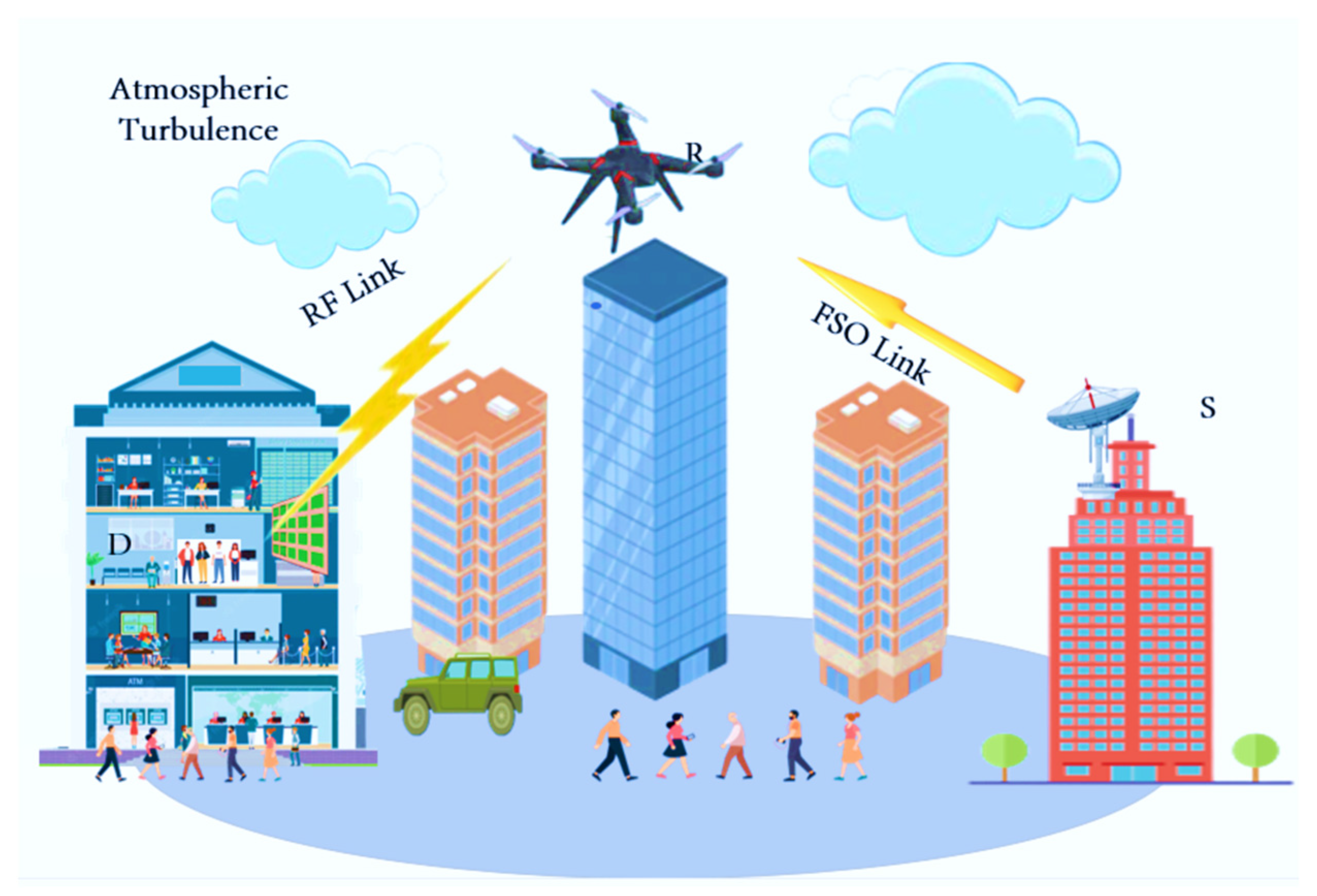
2. System Model

The coverage density in the room affects the connectivity of signal transmission and also makes the window of RIS components small. As described in Section 1, to maximize the spectral efficiency of the system, RIS reflectance and hybrid beamforming design are particularly important. But, due to the non-convexity of this problem, it can be decomposed into two independent optimization sub-problems. The RIS-assisted multiuser millimeter-wave massive MIMO/FSO UAV communication system is shown in Figure 1. The source node (S) communicates with the destination node (D) by decoding forwarding (DF) and relay node (R). The S-R link is equipped with a single antenna, and the R-D link is a millimeter three-wave massive MIMO system model. Node R has optical and RF signal processing capabilities. An incoherent intensity modulation and direct detection (IM/DD) receiver is employed at node R. The power divider separates the electrical signal, which is converted from the incoming optical signal from the alternating current (AC) and coupling (DC) components. An unsolicited DC component, usually filtered out at the receiver, is applied to an energy harvesting unit that provides the collected power to the RF transmitter. The AC component carrying the information is decoded by the decoder circuit. The decoding information is forwarded to the RF transmitter after demodulation according to the RF modulation scheme.

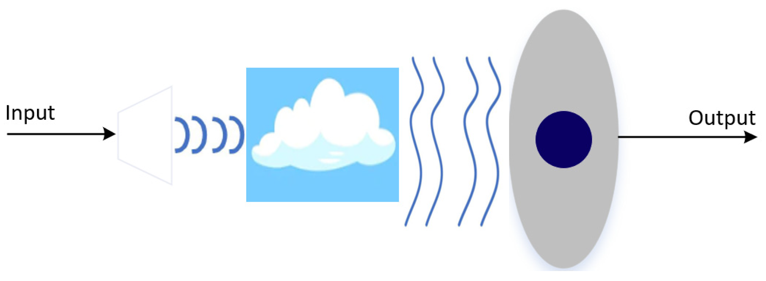
2.1. FSO System Model

The FSO channel between node S and node R is modeled as Gamma-Gamma distribution with PE [8]. The Gamma-Gamma turbulence model characterizes the statistical behavior of received optical irradiance. This model has been widely used in recent literature to simulate FSO channels, depending on its double random scintillation model. The probability distribution function (PDF) of channel coefficient $h_{FSO}$ is given as

$$f_{h_{FSO}}\left(h_{FSO}\right)=\frac{{\varsigma }^2}{h_{FSO}\Gamma \left(\alpha \right)\Gamma \left(\beta \right)}{G}_{\mathrm{1,3}}^{\mathrm{3,0}}\left(\alpha \beta \frac{h_{FSO}}{I_{FSO}{M}_o}{|}_{{\varsigma }^2,\alpha ,\beta }^{{\varsigma }^2+1}\right)$$

(1)

where $\Gamma$(.) is the well-known Gamma function, $G_{p,q}^{m,n}\left({\left.x\right|}_{b_1,\dots ,b_q}^{a_1,\dots ,a_p}\right)$ is the Meijer’s G-function. The AT causes the channel gain of the FSO link to be weakened, denoted as $I_{FSO}$ dealt with S and path loss. Suppose the elements of $I$ are modeled as independent and identically distributed random variables. $\varsigma ={\overline{\omega }}_e/2{\sigma }_s$ is the ratio of equivalent beam radius and zero boresight displacement standard deviation at the photo detector (PD). The constant term $M_o$ is the power fraction received when there is no detector. $1/\alpha$ and $1/\beta$ are the variances of large turbulent vortices and small turbulent vortices, respectively. The FSO system model is shown in Figure 2.

The parameters α and β are distance-dependent fading variables in the presence of AT. Parameter α and β can be expressed as

$$\alpha ={\left\{\mathrm{e}\mathrm{x}\mathrm{p}\left[\frac{0.49{\sigma }_R^2}{{\left(1+1.11{\sigma }_R^{\frac{12}{5}}\right)}^{\frac{7}{6}}}\right]-1\right\}}^{-1}$$

(2)

and

$$\beta ={\left\{exp\left[\frac{0.51{\sigma }_R^2}{{\left(1+0.69{\sigma }_R^{\frac{12}{5}}\right)}^{\frac{5}{6}}}\right]-1\right\}}^{-1}$$

(3)

where ${\sigma }_R^2=1.23C_n^2{v}^{7/6}{d}_{SR}^{11/6}$ represents the Rytov variance, and $C_n^2$, $v$ and $d_{SR}$ represent the refractive index structure constant, wave number, and link length, respectively. $C_n^2$ is typically taken as a value in the range of ${10}^{-17}~{10}^{-13}$ for weak to strong turbulence conditions.

2.2. DF Transmission Protocol

Communication between nodes S and D is performed in two time slots $T_1$ and $T_2$ for the first and second hops, respectively. Relays only harvest energy during $T_1$ because of the increased complexity of the node if power is collected and released at the same time. Node S converts the RF signal vector $r$ with electrical power $\rho$ to an optical signal by employing subcarrier intensity modulation (SIM). The dc bias $A\in [A_{\mathrm{m}\mathrm{i}\mathrm{n}},A_{max}]$ is added to the RF signal to ensure that the optical signal is non-negative, where $A_{min}$ and $A_{max}$ are the minimum and maximum values for the DC bias, respectively. Let $P_{\mathrm{s}}$ indicate the electrical power of node S used to transmit the optical signal vector $s_1$. Then, the optical signal vector can be written as [11]:

$$s_1=\sqrt{P_S}[\delta r+A]$$

(4)

where $\delta$ is the electro-optical conversion coefficient. To avoid clipping problems caused by nonlinearity of semiconductor lasers, the following constraints should be met δ [11]:

$$\delta \le min\left(\frac{A-A_{min}}{\rho },\frac{A_{max}-A}{\rho }\right)$$

(5)

The electrical signal at the output of the PD can be expressed as

$$y_{FSO}=h_{FSO}{s}_1+n_{FSO}$$

(6)

where $h_{FSO}=\left(P_{\mathrm{S}}^2{\eta }^2/{\sigma }_{FSO}^2\right)I_{FSO}$ is the channel coefficient of the S-D link, where $\eta$ is the photoelectric conversion coefficient. The noise in FSO communication systems is expressed as ${\eta }_{FSO}$. ${\eta }_{FSO}$ is caused by circuit noise as well as high-intensity background lighting, and it is often modeled as zero mean additive white Gaussian noise. ${\sigma }_{FSO}^2$ is the variance in the additive white Gaussian noise with a mean of zero.

2.3. Mathematical Modeling of the PE Tracking System

The received electrical SNR with a slow fading channel can be expressed by the following equation [10]:

$$SNR\left(h_{FSO}\right)=\frac{2P_t^2{h}^2{R}^2}{{\sigma }_n^2}$$

(7)

where $h_{FSO}=h_p{h}_d$ includes PE $h_p$ and $h_d$, representing the path loss component caused by other atmospheric attenuation. $h_p$ is an independent random variable. In order to simplify the calculation and analysis, a simplified theoretical model is used in this section, which only considers the direct path loss factor and path attenuation factor of the beam and ignores the influence of AT. The path loss component can be determined by Beer–Lambert’s law as

$$h_d=\mathit{exp}(-{\alpha }_{atmo}z)$$

(8)

where $z$ is the propagation distance and ${\alpha }_{atmo}$ is the attenuation coefficient caused by AT. In the presence of geometric diffusion and PE, the received power of the detector can be expressed by the following equation [10]:

$$h_p\approx A_{0}exp\left(\frac{-2r^2}{w_{zeq}^2}\right)$$

(9)

where $A_0=[erf(v){]}^2$ is the power collected at radial displacement $r=0$. $w_{zeq}^2\widehat{=}{w}_z^2\left(\right(\sqrt{\pi }erf\left(v\right))/(2vexp(-v^2)$ is the equivalent beam width. $v=\sqrt{\pi }a/\sqrt{2}{w}_z$ is the beam width at distance $z$. $a$ is the radius of the detection aperture. The performance of FSO communication under PE can be evaluated based on outage probability.

The performance of the proposed FSO system is provided by the probability of interruption caused by PE. The channel capacity $C\left(h\right)$, which is a measure of the channel’s ability to transmit information, depends on the channel state $h$. The status is affected by factors such as AT and PE. In the proposed FSO system, an interruption occurs when $C\left(h\right)$ is insufficient to support the required data rate $R_0$. And it can be expressed by the following equation:

$$P_{out}\left(R_0\right)=P_r\left(C\right({SNR}_{Rx}\left(h\right))<R_0)$$

(10)

$$\begin{array}{c}{P}_{out}\left(R_0\right)=P_r\left({SNR}_{Rx}\left(h\right)<C^{-1}\left(R_0\right)\right)\\ =P_r(\frac{2P_t^2{h}^2{R}^2}{{\sigma }_n^2}<C^{-1}(R_0\left)\right)\end{array}$$

(11)

The outage probability can be expressed by the following equation:

$$P_{out}=P_r(h<h_0)$$

(12)

where $h_0=\left(\right(\left(C^{-1}\right(R_0\left){\sigma }_n^2\right)/\left(2P_t^2{R}^2\right)){)}^{1/2}$. The outage probability is the cumulative density function of $h$ evaluated as $h_0$. It can be expressed by the following equation:

$$\begin{array}{c}{P}_{out}={\int }_0^{h_0}{f}_{h_p}\left(h_p\right)d{h}_p\\ =k^{\prime }{\int }_0^{h_0}{\left(\ln \left(\frac{A_0}{h_p}\right)\right)}^{m-1}(h_p{)}^{\zeta -1}d{h}_p.\end{array}$$

(13)

On substitution, $x=ln(A_0/h_p)$

$$P_{out}=k^{\prime }{A}_0^{\zeta }{\int }_{\infty }^{\mathit{ln}\left(\frac{A_0}{h_0}\right)}{x}^{m-1}exp(-x\zeta )dx$$

(14)

where

$$k^{\prime }=\frac{{\zeta }^m}{\mathsf{\Gamma }\left(m\right)A_0^{{\zeta }^m}}$$

(15)

Using the approximation of

$${\int }_u^{\infty }{x}^{v-1}exp(-\mu x)dx={\mu }^{-v}\Gamma (v,u\mu )$$

(16)

$$P_{out}=k^{\prime }{A}_0^{\zeta }{\zeta }^{-m}\Gamma (m,\zeta ln(\frac{A_0}{h_0}))$$

(17)

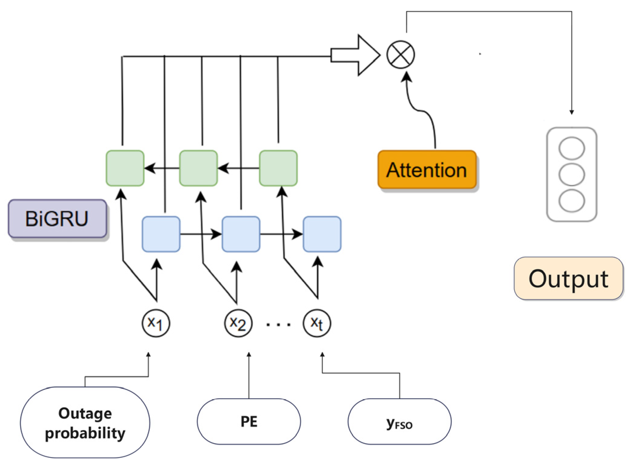
2.4. Estimation of FSO PE with BIGRU-Attention Model

2.4.1. Estimating FSO-PE Using BiGRU-Attention Model

The collimation requirements for airborne communication terminals are higher, with the increase in airborne laser communication distance. Large $s_1$ can lead to large deviations from the laser beam. The application of the BiGRU-Attention neural network model in an FSO system can effectively solve the problem of light PE caused by UAV jitter. $y_{FSO}$, PE, and outage probability are entered into the neural model as parameters corresponding to $x_1$, $x_2$ and $x_3$, respectively.

After the BiGRU-Attention layer, the BiGRU model extracts time-varying information for $y_{\mathrm{F}\mathrm{S}\mathrm{O}}$, PE, and outage probability. The attention mechanism assigns different attention weights to the three sequence parameters. Different weights can distinguish the importance level of different parameters and improve the accuracy of classification, hence effectively solving the problem in FSO.

The BiGRU-Attention model is a bidirectional recursive neural model that simultaneously reads inputs from both ends of the $y_{FSO}$, PE, and interrupts probability parameter time series. The $y_{FSO}$ parameter is the optical signal power of the PD, which represents the signal quality of the free-space optical communication system. This parameter is obtained from the PD measurement on the relay node R. The PE parameter is the angle error between the beam at the transmitter and the receiver. This parameter can be measured by sensors on both the sending and receiving ends. The outage probability is estimated by calculating the number of interruptions in the free-space optical communication link in a certain period. BiGRU-Attention processes all three sequence parameters as inputs.

The BiGRU-Attention model runs on the relay node R. Through a bidirectional mechanism, BiGRU-Attention can capture input parameter information and help extract the features of the entire parameter sequence. According to the bidirectional mechanism characteristics of BiGRU-Attention, it operates in the signal processing unit of the relay node. The signal processing unit of the relay node is connected to each module to obtain the measurement signal $y_{FSO}$ of the photodetector, the error data PE pointing to the sensor, and the outage probability of the statistical unit. The signal processing unit has the function of processing time series signals and can run the BiGRU-Attention model. It connects to the three data sources mentioned above to obtain feature vectors.

After obtaining the results of BiGRU-Attention, the signal processing unit can output the control signal, adjust the beam direction of the transmitter, and complete error correction. This can maximize the effectiveness of the network. This effectively solves the problem of PE in FSO communication systems. The attention mechanism network selects the most critical part of $y_{FSO}$, PE and outage probability parameter time series by learning the attention distribution. This distribution indicates that the network should enhance the critical parameter feature information while decoding.

The BiGRU-Attention model proposed in this paper enters the network through the input and output signals $y_{FSO}$, PE and outage probability as parameters. The BiGRU network learns the parameter time series information. The attention network then emphasizes the importance of key parameter features. Finally, the BiGRU-Attention model effectively solves the pointing error problem in the FSO system.

2.4.2. BiGRU-Attention Model Training and Structure

• Training data

BiGRU-Attention uses historical operating data from a free-space optical communication system as a training set to train the model. The training set includes received optical signal intensity data $y_{FSO}$ measured by photodetectors, real-time angle error data PE recorded by the pointing sensor, and the annualized link outage probability obtained by statistics. $y_{FSO}$ and PE are obtained at a 50 Hz sampling rate, and the network input layer sequence length is set to 200, which is 4 s of data. The data are collected using a custom-built free-space optical communication system, which consists of a transmitter and a receiver. The transmitter includes a laser diode, a beam expander, and a pointing mechanism. The receiver consists of a photo detector, a pointing sensor, and a signal processing unit.

b.

Model structure

BiGRU-Attention consists of an input layer of length 200, two bidirectional GRU hidden layers, and an output layer. The input layer corresponds to the input sequence. Each hidden layer contains 128 nodes. The output layer outputs a pointer to the error correction control signal. The structure of the BiGRU-Attention model is shown in Figure 3.

c.

Training process

Train the network using the AdaGrad optimization algorithm. The learning rate is set to 0.01. The number of training iterations is 1000. The first step is to initialize the BiGRU attention parameters. Then, repeat the training iteration, that is, enter the training sample and calculate the loss through forward propagation. The second step is to calculate the parameter gradient using AdaGrad and update the network parameters with backpropagation until the training loss converges or the number of iteration rounds is reached.

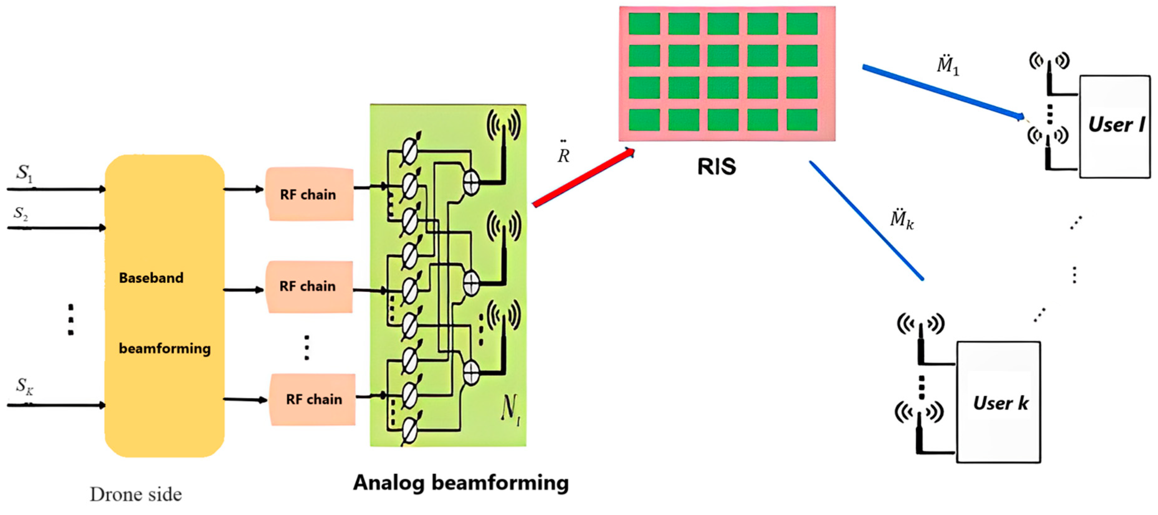
2.5. Multi-User UAV Communication Channel Model with RIS

Figure 4 presents the RIS-assisted multiuser UAV communication system model. The total number of users is expressed in K, and the number of data streams is expressed in $N_{s,K}$. The transmitter for UAVs communication is equipped with two transmitting antennas, denoted by $N_T$, with an $N_T^{RF}$ chain, where $N_{s,K}\le N_T^{RF}\le N_T$. RIS consists of ${\mathcal{T}}^{\mathrm{‘}}$ reflective elements, and the set of reflective elements is expressed as ${\mathcal{T}}^{\mathrm{‘}}=\left\{1,\cdots ,{\mathrm{T}}^{\mathrm{‘}}\right\}$. Typically, RIS can communicate with UAVs using specific links to exchange information about the channel status of the system while allowing for better coordination of the transmission signals of downlinks to multiple users. The reflection coefficient of RIS is expressed as ${\varrho }_{t^{\mathrm{‘}}}=e^{j{\theta }_{t^{\mathrm{‘}}}},\forall t^{\mathrm{‘}}ϵ{\mathcal{T}}^{\mathrm{‘}}$. ${\theta }_{t^{\mathrm{‘}}}ϵ\left[\mathrm{0,2}\pi \right)$ denotes the first $t^{\mathrm{‘}}$ phase shift of the first RIS reflection element. The RIS reflection matrix is expressed as $\Phi =diag\left\{{\varrho }_{1^{‘}},\cdots ,{\varrho }_{{\mathcal{T}}^{‘}}\right\}$, and $\left|{\varrho }_{t^{\mathrm{‘}}}\right|=1,\forall t^{\mathrm{‘}}ϵ{\mathcal{T}}^{\mathrm{‘}}$. Similarly, the phase shift of the RIS reflector satisfies the discrete value ${\theta }_{t^{\mathrm{‘}}}ϵ\mathcal{I}\triangleq \left\{\frac{2\pi \stackrel{⃑}{i}}{2^{\stackrel{⃑}{I}}}|\stackrel{⃑}{i}=\mathrm{0,1},\cdots ,2^{\stackrel{⃑}{I}}-1\right\}$. $\mathcal{I}$ represents the resolution of each reflector.

Let $s_1=\sqrt{P_R}{y}_{FSO}$ denote the signal forwarded by the node R. For this system, for K terrestrial users, the signal first enters the digital signal vector through the baseband beamforming matrix $F_{BB}$. Then, the simulated beamforming matrix $F_{RF}$ obtains the UAV transmit signal as:

$$x={\sum }_{k=1}^K{F}_{RF}{F}_{BB,k}{s_1}_k$$

(18)

where $F_{RF}ϵ{\mathbb{C}}^{N_T\times N_{RF}^T}$, $F_{BB,k}=\left[F_{BB,1},\cdots F_{BB,K}\right]ϵ{\mathbb{C}}^{N_{RF}^T\times N_{s,k}}$, $N_{s,k}={\sum }_{k=1}^K{N}_{s,k}$. ${s_1}_k={\left[s_1^T,\cdots ,s_K^T\right]}^Tϵ{\mathbb{C}}^{N_s\times 1}$ represents the connection of a single user’s parallel data stream. ${\mathit{s}}_kϵ{\mathbb{C}}^{N_{S,k}\times 1}$ denotes the first $k$ Gaussian encoded data stream vector for the first user satisfying $\mathbb{E}\left[s_k{s}_k^H\right]=I_{N_{s,k}}$. The maximum signal transmission power $P$ satisfies ${‖F_{RF}{F}_{BB}‖}_F^2\le P$.

The UAV transmits a communication signal to the RIS, and the RIS passes the communication signal to the user. The user is equipped with $N_R$ receiving antennas and $N_R^{RF}$ RF chains, where ${N_{S,k}\le N}_R^{RF}\le N_R$. For signal accuracy, an analog combiner matrix is designed as $W_{RF,k}$ and a digital combiner matrix $W_{BB,k}(W_{RF,k}ϵ{\mathbb{C}}^{N_R\times N_{RF}^R}$ and $W_{BB,k}ϵ{\mathbb{C}}^{N_{RF}^R\times N_{s,k}}$). Therefore, the received signal $y_k\in {\mathbb{C}}^{{\mathsf{{\rm N}}}_{s,k}\times 1}$ at the kth terrestrial user can be expressed by the following equation:

$$\begin{array}{c}{y}_k\left(t\right)=W_{BB,k}^H{W}_{RF,k}^H({\ddot{M}}_k\left(t\right){\Phi \ddot{R}\left(t\right))F}_{RF}{F}_{BB,k}{s}_k\\ +W_{BB,k}^H{W}_{RF,k}^H{\left({\ddot{M}}_k\left(t\right)\Phi \ddot{R}\left(t\right)\right)\sum _{j\ne k,jϵ\mathcal{K}}{W}_{BB,k}^H{W}_{RF,k}^H{F_{RF}F}_{BB,k}{s}_k+W_{BB,k}^H{W}_{RF,k}^{H}n}_k\left(t\right)\end{array}$$

(19)

where $W_{BB,k}^H{W}_{RF,k}^H({\ddot{M}}_k\left(t\right){\Phi \ddot{R}\left(t\right))F}_{RF}{F}_{BB,k}{s}_k$ represents the received signal excluding other interference. $W_{BB,k}^H{W}_{RF,k}^H{\left({\ddot{M}}_k\left(t\right)\Phi \ddot{R}\left(t\right)\right)\sum _{j\ne k,jϵ\mathcal{K}}{W}_{BB,k}^H{W}_{RF,k}^H{F_{RF}F}_{BB,k}{s}_k}_{}$ is the interference signal, and $W_{BB,k}^H{W}_{RF,k}^H{n}_k$ represents the total noise. $F_{BB,k}ϵ{\mathbb{C}}^{N_{RF}^T\times N_{s,k}}$ and $F_{RF}ϵ{\mathbb{C}}^{N_T\times N_{RF}^T}$ represent the baseband beamforming matrix and the analog beamforming matrix, respectively. $n_k~\mathcal{C}\mathcal{N}\left(0,{\delta }^{2}I\right)$ is the $k$ additive Gaussian white noise at the user. ${\ddot{M}}_k\left(t\right)$ is the millimeter-wave large-scale channel matrix from the RIS to the user. $\ddot{R}\left(t\right)$ is the millimeter-wave large-scale channel matrix from the UAV to the RIS. ${\ddot{M}}_k\left(t\right)$ and $\ddot{R}\left(t\right)$ are defined as follows:

$${\ddot{M}}_k\left(t\right)=\sqrt{\frac{{{\mathrm{T}}^{\mathrm{‘}}N}_R}{Q_{{\ddot{M}}_k}}}\sum _{q=1}^{Q_{{\ddot{M}}_k}}{\stackrel{̿}{\kappa }}_{km,q}\left(t\right){\stackrel{̿}{\alpha }}_R\left({{\phi }_{km,q}}^R\left(t\right)\right){\stackrel{̿}{\alpha }}_{P_1}^H\left({{\phi }_{km,q}}^T\left(t\right),{{\eta }_{km,q}}^T\left(t\right)\right)ϵ{\mathbb{C}}^{N_R\times {\mathrm{T}}^{\mathrm{‘}}}$$

(20)

$$\ddot{R}\left(t\right)=\sqrt{\frac{{{\mathrm{T}}^{\mathrm{‘}}N}_T}{Q_{\ddot{R}}}}\sum _{q=1}^{Q_{\ddot{R}}}{\stackrel{̿}{\kappa }}_{r,q}\left(t\right){\stackrel{̿}{\alpha }}_{P_2}\left({{\phi }_{r,q}}^R\left(t\right),{{\eta }_{r,q}}^R\left(t\right)\right){\stackrel{̿}{\alpha }}_T^H\left({{\nu }_{r,q}}^T\left(t\right)\right)ϵ{\mathbb{C}}^{{\mathrm{T}}^{\mathrm{‘}}\times N_T}$$

(21)

The UAV and the user are equipped with uniform linear arrays. RIS is equipped with a uniform planar array of size ${T^{‘}}_y\times {T^{‘}}_z$. $Q_{{\ddot{M}}_k}$ and $Q_{\ddot{R}}$ are the numbers of channel paths from the RIS to the $k$ user and the number of channel paths between the UAV and the RIS. ${\stackrel{̿}{\kappa }}_{km,q}\left(t\right)$ denotes the path gain from the RIS to the $k$ user, and the path gain ${\stackrel{̿}{\kappa }}_{r,q}\left(t\right)$ denotes the fast fading path gain between the UAV and the RIS. ${\stackrel{̿}{\alpha }}_R\left({{\phi }_{km,q}}^R\left(t\right)\right)$, ${\stackrel{̿}{\alpha }}_T\left({{\nu }_{r,q}}^T\left(t\right)\right)$, ${\stackrel{̿}{\alpha }}_{P_1}\left({{\phi }_{km,q}}^T\left(t\right)\right)$, ${{\eta }_{km,q}}^T\left(t\right)$ and ${\stackrel{̿}{\alpha }}_{P_2}({{\phi }_{r,q}}^R\left(t\right),{{\eta }_{r,q}}^R\left(t\right))$ are the steering vectors corresponding to the uniform linear array and the uniform planar array, respectively.

$${\stackrel{̿}{\alpha }}_R\left({{\phi }_{km,q}}^R\left(t\right)\right)=\frac{1}{\sqrt{N_R}}\left[1,\dots ,e^{j\left(N_R-1\right)d\mathit{sin}\left({{\phi }_{km,q}}^R\left(t\right)\right)\frac{2\pi }{\lambda }}\right]$$

(22)

$${\stackrel{̿}{\alpha }}_T\left({{\nu }_{r,q}}^T\left(t\right)\right)=\frac{1}{\sqrt{N_T}}\left[1,\dots ,e^{j\left(N_T-1\right)d\mathit{sin}\left({{\phi }_{km,q}}^T\left(t\right)\right)\frac{2\pi }{\lambda }}\right]$$

(23)

$$\begin{array}{c}{\stackrel{̿}{\alpha }}_{P_1}\left({{\phi }_{km,q}}^T\left(t\right),{{\eta }_{km,q}}^T\left(t\right)\right)\\ =\frac{1}{\sqrt{M_y{M}_z}}\left[1,\dots ,e^{jd\mathit{sin}\left(\left(M_y-1\right)\mathit{sin}\left({{\phi }_{km,q}}^T\left(t\right)\right)\mathit{sin}\left({{\eta }_{km,q}}^T\left(t\right)\right)+\left(M_z-1\right)\mathit{cos}\left({{\phi }_{km,q}}^T\left(t\right)\right)\right)\frac{2\pi }{\lambda }}\right]\end{array}$$

(24)

$$\begin{array}{c}{\stackrel{̿}{\alpha }}_{P_2}\left({{\phi }_{r,q}}^R\left(t\right),{{\eta }_{r,q}}^R\left(t\right)\right)\\ =\frac{1}{\sqrt{M_y{M}_z}}\left[1,\dots ,e^{jd\mathit{sin}\left(\left(M_y-1\right)\mathit{sin}\left({{\phi }_{r,q}}^R\left(t\right)\right)\mathit{sin}\left({{\eta }_{r,q}}^R\left(t\right)\right)+\left(M_z-1\right)\mathit{cos}\left({{\eta }_{r,q}}^R\left(t\right)\right)\right)\frac{2\pi }{\lambda }}\right]\end{array}$$

(25)

where $d=\frac{\lambda }{2}$ is the antenna spacing and $\lambda$ is the signal wavelength.

3. Power Fading Factor and Doppler Shift estimation for Fast Fading Channels Based on Tensor-Train Decomposition

3.1. Tensor-Train Decomposition

Tensor-train is a higher-order tensor decomposition that represents a higher-order tensor as a product of several lower-order tensors. Tensor-train decomposition is an effective method for compressed representation of high-dimensional data that can reduce the number of dimensions and simplify the computation while maintaining the main structure of the data. It is very useful in dealing with large-scale high-dimensional data. The main benefit of the Tensor-train method is the ability to obtain a low-dimensional representation of the high-dimensional signal by Tensor-train decomposition, which simplifies the dimensionality and improves the robustness. Thus, Tensor-train helps to improve the accuracy of parameter estimation for power fading and Doppler shift.

$\mathcal{X}$ is an nth order tensor of size $I_1\times \cdots \times I_N$. Its Tensor-train representation uses N tensor cores ${\mathcal{G}}_1,{\mathcal{G}}_2,\cdots ,{\mathcal{G}}_N$, where the size of each tensor core is $R_{n-1}\times I_n\times R_n$, $R_0=R_N=1$.

$$\mathcal{X}=\sum _{r_1=1}^{R_1}\sum _{r_2=2}^{R_2}\cdots \sum _{r_{N-1}=1}^{R_{N-1}}{\mathcal{G}}_1\left(:,r_1\right)\circ {\mathcal{G}}_2\left(r_1,:,r_2\right)\circ \cdots \circ {\mathcal{G}}_{N-2}\left(r_{N-2},:,r_{N-1}\right)\circ {\mathcal{G}}_N\left(r_{N-1},:\right)$$

(26)

A Tensor-train $\mathcal{Y}={\mathcal{G}}_1\circ {\mathcal{G}}_2·\cdots \circ {\mathcal{G}}_N$ of rank $\left(R_0,R_1,\cdots R_N\right)$ has rank $R_1{R}_2\cdots R_{N-1}$, and the equivalent Kruskal tensor is denoted as $\mathcal{Y}=⟦A^{\left(1\right)},A^{\left(2\right)},\cdots A^{\left(N\right)}⟧$, where $A^{\left(n\right)}$ is given by the following equation:

$$A^{\left(n\right)}={\left[{\mathcal{G}}_n\right]}_{\left(2\right)}\left(I_{R>n}^T⨂I_{R_{n-1}{R}_n}⨂I_{R<n-1}^T\right)$$

(27)

where $R_{<n}=R_0{R}_1\cdots R_{n-1}$ $R_{>n}=R_{n+1}\cdots R_{N-1}{R}_N$.

3.2. Estimation of Power Fading Factor and Doppler Shift for Fast-Fading Channels Using Tensor-Train Decomposition

The received signal at the single-user of a millimeter-wave MIMO in a UAV can be expressed as the following equation:

$$\begin{array}{c}{y}_k\left(t\right)=W_{BB,k}^H{W}_{RF,k}^H\sqrt{\frac{{T^{‘}N}_R}{Q_{{\ddot{M}}_k}}}\sum _{q=1}^{Q_{{\ddot{M}}_k}}{\stackrel{̿}{\kappa }}_{km,q}\left(t\right){\stackrel{̿}{\alpha }}_R\left({{\phi }_{km,q}}^R\left(t\right)\right){\stackrel{̿}{\alpha }}_{P_1}^H\left({{\phi }_{km,q}}^T\left(t\right),{{\eta }_{km,q}}^T\left(t\right)\right)F_{RF}{F}_{BB,k}{s}_k\\ +{\left(W_{RF}{W}_{BB}\right)}^H\overleftarrow{N}\left(t\right)\end{array}$$

(28)

Set the conversion again as follows: $\sqrt{\frac{N_T{N}_R}{Q}}$ is a constant, namely $\sqrt{\frac{N_T{N}_R}{Q}}=1$.

$${\tilde{\alpha }}_R\left({{\phi }_{km,q}}^R\left(t\right)\right)=W_{BB,k}^H{W}_{RF,k}^H{\stackrel{̿}{\alpha }}_R\left({{\phi }_{km,q}}^R\left(t\right)\right)ϵ{\mathbb{C}}^{N_{RF}^R\times 1}$$

(29)

$${\tilde{\alpha }}_P\left({{\eta }_{km,q}}^T\left(t\right)\right)={\stackrel{̿}{\alpha }}_{P_1}^H\left({{\phi }_{km,q}}^T\left(t\right),{{\eta }_{km,q}}^T\left(t\right)\right){\ddot{\mathsf{\Phi }R}\left(t\right)F}_{RF}{F}_{BB,k}{s}_kϵ{\mathbb{C}}^{N_{RF}^T\times 1}$$

(30)

where ${\tilde{\alpha }}_R\left({{\phi }_{km,q}}^R\left(t\right)\right)$ and ${\tilde{\alpha }}_P\left({{\eta }_{km,q}}^T\left(t\right)\right)$ represent the receive vector and the send vector, respectively. Equation (28) is expressed as the following equation:

$$\mathrm{Y}\left(t\right)=\sum _{q=1}^{Q_{{\ddot{M}}_k}}{\stackrel{̿}{\kappa }}_{km,q}\left(t\right){\tilde{\alpha }}_R\left({{\phi }_{km,q}}^R\left(t\right)\right){\tilde{\alpha }}_P\left({{\eta }_{km,q}}^T\left(t\right)\right)+{\left(W_{RF}{W}_{BB}\right)}^H\overleftarrow{N}\left(t\right)$$

(31)

The received signal tensor for T consecutive time slots as a rank-one vector accumulation pattern is expressed as the following equation:

$$\mathcal{Y}=\sum _{q=1}^Q\mathcal{T}{\tilde{\alpha }}_R\left({{\beta }_q}^R\left(t\right)\right)·{\tilde{\alpha }}_T\left({{\gamma }_q}^T\left(t\right)\right)·{\tilde{\kappa }}_q\left(t\right)+\mathcal{N}$$

(32)

where $\mathcal{T}$ is the weight of the multiplication of the rank-one factors. $\mathcal{Y}\mathsf{ϵ}{\mathbb{C}}^{N_{RF}^R\times N_{RF}^T\times T}$ is the received signal tensor. ${\tilde{\kappa }}_q\left(t\right)={\left[{\kappa }_q\left(1\right),\cdots ,{\kappa }_q\left(T\right)\right]}^Tϵ{\mathbb{C}}^{T\times 1}$ is the vector containing the fast-fading coefficients from T consecutive time slots. $\mathcal{N}ϵ{\mathbb{C}}^{N_{RF}^R\times N_{RF}^T\times T}$ is the noise tensor. Meanwhile, Equation (32) can continue to be expressed as a Tensor-train decomposition of the $Kruskal$form as follows:

$$\mathcal{Y}=\mathcal{T};U_1,U_2,U_3+\mathcal{N}$$

(33)

$$U_1=\left[{\tilde{\alpha }}_R\left({{\beta }_1}^R\left(t\right)\right),\cdots ,{\tilde{\alpha }}_R\left({{\beta }_Q}^R\left(t\right)\right)\right]\in {\mathbb{C}}^{N_{RF}^R\times Q}$$

(34)

$$U_2=\left[{\tilde{\kappa }}_1\left(t\right),\cdots {\tilde{\kappa }}_Q\left(t\right)\right]\in {\mathbb{C}}^{N_{RF}^T\times Q}$$

(35)

$$U_3=\left[{\tilde{\alpha }}_T\left({{\gamma }_1}^T\left(t\right)\right),\cdots {\tilde{\alpha }}_T\left({{\gamma }_Q}^T\left(t\right)\right)\right]\in {\mathbb{C}}^{\mathrm{T}\times Q}$$

(36)

The FCTPM based on tensor decomposition is utilized by the power method (PM) for the auxiliary unfolding matrix decomposition. FCTPM is based on a combination of Tensor-train decomposition and power. The FCTPM approximates the most dominant rank-negative-one tensor of the input tensor by the Tensor-train decomposition. Each unfolding matrix is also decomposed using a rank-negative-one matrix decomposition. This property allows each unfolding matrix to ignore the concatenation between other unfolding matrices. Therefore, a cyclic update method is proposed to consider the connectivity between the unfolding matrices. After all of the left singular vectors have been computed, the order of the update steps for the right singular vectors needs to be changed. FCTPM utilizes the PM for the auxiliary unfolding matrix decomposition. Therefore, the PM ensures the convergence of the decomposition factors. The cyclic updating method enhances the connectivity between the decomposition factors.

The FCTPM consists of two main components, namely the rank-negative-one tensor approximated by the Tensor-train decomposition of the auxiliary expansion matrix and the PM of determining the left and right singular vectors obtained from the randomly initialized vectors. The core tensor ${\mathcal{G}}^{\left(n\right)}$ calculation in Tensor-train decomposition is based on low-rank approximation of the auxiliary matrix of N-dimensional input tensor $\mathcal{Y}\in {\mathbb{R}}^{I_1\times \cdots I_N}$, and $R_N$ denotes the Tensor-train rank in Tensor-train decomposition of the received signal tensor $\mathcal{Y}$. In FCTPM, a rank-negative-one approximation is made to the high-dimensional input tensor using the Tensor-train decomposition. The received signal at the user is compressed into a low-order core tensor ${\mathcal{G}}^{\left(1\right)}$, ${\mathcal{G}}^{\left(2\right)}$, and ${\mathcal{G}}^{\left(3\right)}$ of the concatenation. The received signal tensor $\mathcal{Y}$ is written in the following form:

$$\begin{array}{c}\mathcal{Y}=\sum _{r_1=1}^{R_1}\cdots \sum _{r_2=1}^{R_2}{\mathcal{G}}_{r_0,:,r_1}^{\left(1\right)}\circ {\mathcal{G}}_{r_1,:,r_2}^{\left(2\right)}\circ {\mathcal{G}}_{r_2,:,r_3}^{\left(3\right)}+\mathcal{N}\\ ={\mathcal{G}}_{1,:,1}^{\left(1\right)}\circ {\mathcal{G}}_{1,:,1}^{\left(2\right)}\circ {\mathcal{G}}_{1,:,1}^{\left(3\right)}+\mathcal{N}\\ =g^{\left(1\right)}\circ g^{\left(2\right)}\circ g^{\left(3\right)}+\mathcal{N}\end{array}$$

(37)

where ${\mathcal{G}}^{\left(n\right)}$ denotes the core tensor of size $R_{n-1}\times I_n\times R_n$ of the core tensor of the rank-negative-one Tensor-train, with all elements of the Tensor-train rank being 1. Then, ${\mathcal{G}}^{\left(n\right)}$ size become $1\times I_n\times 1$ the core tensor of the rank-negative-one Tensor-train. Furthermore, if the core tensor ${\mathcal{G}}^{\left(n\right)}$ of dimensionality is compressed, the core tensor can be regarded as factored vector data $g^{\left(n\right)}ϵ{\mathbb{R}}^{I_n}$ where $g^{\left(n\right)}$ is the rank-negative-one Tensor-train core tensor ${\mathcal{G}}_{1,:,1}^{\left(n\right)}$ of the first-order factor vector.

To solve the factor vector $g^{\left(n\right)}$, Equation (32) is expressed as the following Equation (38):

$$\begin{array}{c}\underset{g^{\left(1\right)},g^{\left(2\right)},g^{\left(3\right)}}{\min }{‖\mathcal{Y}-d{g}^{\left(1\right)}\circ g^{\left(2\right)}\circ g^{\left(3\right)}‖}^2\\ s_{.}{t}_{.}\hspace{1em}d>0,{g^{\left(n\right)}}^T{g}^{\left(n\right)}=1\left(n=\mathrm{1,2},3\right)\end{array}$$

(38)

where $d$ is the principal singular value of the approximate rank-negative-one tensor. According to FCTPM, the higher-order tensor is decomposed in the Tensor-train decomposition by a low-rank decomposition of the auxiliary expansion matrix of the input tensor.

The solution to the factor vector $g^{\left(n\right)}$ can be solved in a uniform manner by expressing:

$$\begin{array}{c}\underset{g^{\left(N-1\right)},g^{\left(N\right)}}{\min }{‖Y_{〈N-1〉}-d^{\left(N-1\right)}{g}^{\left(N-1\right)}{g^{\left(N\right)}}^T‖}_F^2\\ s_{.}{t}_{.}\hspace{1em}d>0,{g^{\left(N-1\right)}}^T{g}^{\left(N-1\right)}=1,{g^{\left(N\right)}}^T{g}^{\left(N\right)}=1\end{array}$$

(39)

where $Y_{〈N-1〉}=reshape\left(v^{\left(N-2\right)},\left[I_{N-1},I_N\right]\right), d^{\left(N-1\right)}$ is the principal singular value after reshaping the matrix. The principal singular value of the rank-negative-one tensor can be calculated as $d=\prod _{i=1}^{N-1}{d}^{\left(i\right)}$, which is the corresponding factor vector. $g^{\left(N-1\right)}$ and $g^{\left(N\right)}$ are the corresponding factor vectors, from which the factor vector can then be composed to derive the corresponding factor matrix. The solution process is repeated until the right singular vector in the decomposition process $v^{\left(N-1\right)}$ is the last factor vector $g^{\left(N\right)}$. Therefore, the first factor vector $g^{\left(1\right)}$ can be expressed as follows:

$$\begin{array}{c}\underset{g^{\left(1\right)},v}{\min }{‖Y_{〈1〉}-d^{\left(1\right)}{g}^{\left(1\right)}{v^{\left(1\right)}}^T‖}_F^2\\ s_{.}{t}_{.}\hspace{1em}{d}^{\left(1\right)}>0,{g^{\left(1\right)}}^T{g}^{\left(1\right)}=1,{v^{\left(1\right)}}^T{v}^{\left(1\right)}=1\end{array}$$

(40)

where $Y_{〈1〉}$ is modulo 1 expansion matrix, $d^{\left(1\right)}$ is the principal singular value of $Y_{〈1〉}$, and $g^{\left(1\right)}$ represents the first factor vector of the rank-negative-one Tensor-train decomposition. $v^{\left(1\right)}$ is the right singular vector of $Y_{〈1〉}$. After obtaining $g^{\left(1\right)}$, $v^{\left(1\right)}$ is expressed as the modulo 2 expansion matrix form of the received signal tensor $\mathcal{Y}$. The second factor vector $g^{\left(2\right)}$ is calculated as:

$$Y_{〈2〉}=reshape\left(v^{\left(1\right)},\left[I_2,\prod _{j=3}^N{I}_j\right]\right)$$

(41)

The rank-negative-one matrix decomposition for $Y_{〈2〉}$ is expressed as the following equation:

$$\begin{array}{c}\underset{g^{\left(2\right)},v^{\left(2\right)}}{\min }{‖Y_{〈2〉}-d^{\left(2\right)}{g}^{\left(2\right)}{v^{\left(2\right)}}^T‖}_F^2\\ s_{.}{t}_{.}{d}^{\left(2\right)}>0,{g^{\left(2\right)}}^T{g}^{\left(2\right)}=1,{v^{\left(2\right)}}^T{v}^{\left(2\right)}=1\end{array}$$

(42)

where $d^{\left(2\right)}$ is the principal singular value of the tensor $\mathcal{Y}$ modulo 2 matrices $Y_{〈2〉}$, and $g^{\left(2\right)}$ represents the second factor vector of the rank-negative-one Tensor-train decomposition. Similarly, the third factor vector can be obtained. This computation can be performed repeatedly until the right singularity vector of the decomposition process is the last factor vector. To ensure convergence of the factorization, a matrix factorization method PM is incorporated. In solving the first-factor matrix, the PM method initializes the factor vector $g^{\left(1\right)}$ to a random unit vector satisfying ${‖g^{\left(1\right)}‖}_2=1$. After that, the vector-matrix operation is performed iteratively until the factor vectors satisfy the pre-set specific termination conditions, as shown below:

$$v^{\left(1\right)}=\frac{Y_{〈1〉}^T{g}^{\left(1\right)}}{{‖Y_{〈1〉}^T{g}^{\left(1\right)}‖}_2}ϵ{\mathbb{R}}^{\prod _{j=2}^N{I}_j}$$

(43)

$$g^{\left(1\right)}=\frac{Y_{〈1〉}{v}^{\left(1\right)}}{{‖Y_{〈1〉}{v}^{\left(1\right)}‖}_2}ϵ{\mathbb{R}}^{I_1}$$

(44)

where $g^{\left(1\right)}$ and $v^{\left(1\right)}$ are $Y_{〈1〉}$ the left and right singular vectors, respectively. The main singular value $d^{\left(1\right)}$ associated with it can be expressed as $d^{\left(1\right)}={g^{\left(1\right)}}^T{Y}_{〈1〉}{v}^{\left(1\right)}$. The left singular vector calculation follows immediately after the right singular vector calculation. Assuming the existence of an orthogonal basis $\overline{U}ϵ{\mathbb{R}}^{I_1\times R}$ and $\overline{V}ϵ{\mathbb{R}}^{I_2\cdots I_N\times R}$, the unfolding matrix $Y_{〈1〉}$ satisfies the following equation:

$$Y_{〈1〉}=\sum _{j=1}^R{d}_j{\overline{U}}_{:,j}{\overline{V}}_{:,j}^T$$

(45)

where $d_j$ is the singular value of the singular vector, which corresponds to $Y_{〈1〉}$. After several iterations, $v^{\left(1\right)}$ and $g^{\left(1\right)}$ can be defined by the following equations, respectively:

$$v^{\left(1\right)}={\delta }_{v^{\left(1\right)}}\sum _{j=1}^R{d}_j^{2k+1}{\overline{V}}_{:,j}{\overline{U}}_{:,j}^T{g}^{\left(1\right)}$$

(46)

$$g^{\left(1\right)}={\delta }_{g^{\left(1\right)}}\sum _{j=1}^R{d}_j^{2k}{\overline{U}}_{:,j}{\overline{U}}_{:,j}^T{g}^{\left(1\right)}$$

(47)

where ${\delta }_{g^{\left(1\right)}}$ and${\delta }_{v^{\left(1\right)}}$ are the corresponding normalization factors. Thus, after several iterations of PM, $v^{\left(1\right)}$ and $g^{\left(1\right)}$ satisfy $\frac{{‖v^{\left(1\right)}‖}_2^2}{{‖g^{\left(1\right)}‖}_2^2}=1$ by the convergence property, and the $\frac{{\delta }_{v^{\left(1\right)}}}{{\delta }_{g^{\left(1\right)}}}$ converges to the maximum singular value $d_1$, at $Y_{〈1〉}^T{g}^{\left(1\right)}=\left(\frac{{\delta }_{v^{\left(1\right)}}}{{\delta }_{g^{\left(1\right)}}}\right)v^{\left(1\right)}$, ${‖Y_{〈1〉}^T{g}^{\left(1\right)}-d_1{v}^{\left(1\right)}‖}_2=0$.

From the previous rank-negative-one Tensor-train decomposition, the nth factor vector $g^{\left(n\right)}$ depends on the previously computed right singular vector $v^{\left(n-1\right)}$, while $v^{\left(n-1\right)}$ is obtained from the computed n−1 factor vector $g^{\left(n-1\right)}$, because the matrix decomposition of each factor vector is performed independently. These properties can lead to problems with local optimization, resulting in a loss of critical performance in FCTPM. To enhance the connectivity between the decomposition factors, a circular update method is proposed, which changes the order in which the left singular vectors are computed. According to the decomposition method of Tensor-train of rank-negative-one and the nature of PM, $v^{\left(n\right)}$ can be obtained from $g^{\left(n+1\right)}$ and $v^{\left(n+1\right)}$, which are reshaped to form $v^{\left(n\right)}$. The relationship $g^{\left(n\right)}$ is updated in the following way:

$$\begin{array}{c}{v}^{\left(n\right)}\approx {\widehat{v}}^{\left(n\right)}=reshape\left(d^{\left(n+1\right)}{g}^{\left(n+1\right)}{v^{\left(n+1\right)}}^T,\left[I_{n+1}\cdots I_N\right]\right)\\ g^{\left(n\right)}=\frac{{\mathcal{Y}}_{〈n〉}{\widehat{v}}^{\left(n\right)}}{{‖{\mathcal{Y}}_{〈n〉}{\widehat{v}}^{\left(n\right)}‖}_2}\end{array}$$

(48)

The updated factor vector $g^{\left(2\right)}$ can be derived as $g^{\left(2\right)}=\frac{{\mathcal{Y}}_{〈2〉}{\widehat{v}}^{\left(2\right)}}{{‖{\mathcal{Y}}_{〈2〉}{\widehat{v}}^{\left(2\right)}‖}_2}$.

The channel parameter is estimated for the UAV with millimeter-wave massive MIMO based on the FCTPM. The number of factor matrix time slots is associated with the structure of the transmission frame, using a downlink transmission frame structure. It consists of an AOA/AOD estimation phase ($T_1$ time slot), a fast-fading factor estimation phase ($T_2$ time slot), and the data transmission phase ($T_3$ time slot). Using Equations (32) and (33), the received signal at the terrestrial user is represented as the following equation:

$${\mathcal{Y}}^{T_2}=\mathcal{T};U_1,U_2,U_3+{\mathcal{N}}^{T_2}$$

(49)

Matrix $\left\{U_1,U_2,U_3\right\}$ is the received signal at the user. $\mathcal{Y}$ corresponds to the matrix of three factors. $U_2$ is the corresponding fast-fading factor matrix. From the Tensor-train decomposition’s $Kruskal$ representation, $U_n$ and ${\mathcal{G}}_n$, the correspondence can be expressed by the following equation:

$$\begin{array}{c}{U}_n={\left[{\mathcal{G}}_n\right]}_{\left(2\right)}\left(1_{R_{>\left(n\right)}}^T⨂{\mathsf{{\rm I}}}_{R_{n-1}}{R}_n⨂1_{R_{<n-1}}^T\right),n=\mathrm{1,2},3\\ ={\left[g^{\left(n\right)}\right]}_{\left(2\right)}\left(1_{R_{>\left(n\right)}}^T⨂{\mathsf{{\rm I}}}_{R_{n-1}}{R}_n⨂1_{R_{<n-1}}^T\right),n=\mathrm{1,2},3\end{array}$$

(50)

The factor matrix $U_2={\left[g^{\left(n\right)}\right]}_{\left(2\right)}\left(1_{R_{>\left(2\right)}}^T⨂{\mathsf{{\rm I}}}_{R_1}{R}_n⨂1_{R_1}^T\right)$. From Equation (35), we can find that the factor matrix $U_2$ has the fast-fading channel power fading factor associated with the Doppler shift in its elements. We can derive the fast-fading channel power factor. We can obtain $U_2=\left[{\tilde{\kappa }}_1,\cdots {\tilde{\kappa }}_Q\right]ϵ{\mathbb{C}}^{T_2\times Q}$, ${\tilde{\kappa }}_Q={\left[{\tilde{\kappa }}_1\left(1\right),\cdots {\tilde{\kappa }}_Q\left(T_2\right)\right]}^Tϵ{\mathbb{C}}^{T_2\times 1}$. According to the correlation scheme, the Doppler shift on the $q$ path is solved as follows:

$${\widehat{f}}_q=\underset{f_{\mathrm{q}}}{\mathrm{argmax}}\frac{\left|[{\widehat{U}}_2{]}_{:,q}^H\kappa \left(f_{\mathrm{q}}\right)\right|}{{‖[{\widehat{U}}_2{]}_{:,q}‖}_2{‖\kappa \left(f_{\mathrm{q}}\right)‖}_2}.1\le \mathrm{q}\le Q.{\widehat{f}}_q\in [0,f_{max}]$$

(51)

$$f_{max}=\frac{f_c{v}^{\prime }}{c}{\kappa }_q\left(t\right)=b_q{e}^{j2\pi f_{q}t}$$

(52)

where $f_{max}$ is the maximum Doppler shift, $f_c$ is the carrier frequency, $v^{\prime }$ is the speed of the drone, and $c$ is the speed of light. The path gain is estimated from the estimated Doppler shift.

$${\widehat{b}}_q=[\kappa \left({\widehat{f}}_q\right){]}^{\uparrow }[{\widehat{U}}_2{]}_{:,q}$$

(53)

Finally, all parameters of the time-varying channel of the millimeter-wave MIMO in UAV are estimated, and the channel matrix can be recovered from (51).

4. Hybrid Beamforming and RIS Phase Shift Matrix Design

4.1. Hybrid Beamforming and RIS Phase Shift Matrix Design Based on Tensor-Train Decomposition

Define $\sqrt{\frac{{{\mathrm{T}}^{\mathrm{‘}}N}_R}{Q_{{\ddot{M}}_k}}}$ and $\sqrt{\frac{{{\mathrm{T}}^{\mathrm{‘}}N}_T}{Q_{\ddot{R}}}}$ as constants and set them to 1. The millimeter-wave massive channel from the RIS to the user side ${\ddot{M}}_k$ and the millimeter wave massive channel from the UAV side to the RIS $\ddot{R}$ can be written with Tensor-train decomposition form as follows, respectively.

$$\begin{array}{c}{\ddot{\mathcal{M}}}_k={\displaystyle \sum _{q=1}^{Q_{{\ddot{M}}_k}}}\mathcal{T}{\stackrel{̿}{\kappa }}_{km,q}·{\stackrel{̿}{\alpha }}_R\left({{\phi }_{km,q}}^R\left(t\right)\right)·{\stackrel{̿}{\alpha }}_{P_1}^H\left({{\phi }_{km,q}}^T\left(t\right),{{\eta }_{km,q}}^T\left(t\right)\right)\\ =\mathcal{T};{\stackrel{̿}{A}}_{R,km},{\stackrel{̿}{\mathsf{\Lambda }}}_{km,q},{\stackrel{̿}{A}}_{P_1,km}^H\\ ={\stackrel{̿}{g}}_{R,km}^{\left(1\right)}\circ {\stackrel{̿}{g}}_{km,q}^{\left(2\right)}\circ {\stackrel{̿}{g}}_{P_1,km}^{H\left(3\right)}\end{array}$$

(54)

$$\begin{array}{c}\ddot{\mathcal{R}}={\displaystyle \sum _{q=1}^{Q_{\ddot{R}}}}{\mathcal{T}\stackrel{̿}{\kappa }}_{r,q}\left(t\right)·{\stackrel{̿}{\alpha }}_{P_2}\left({{\phi }_{r,q}}^R\left(t\right),{{\eta }_{r,q}}^R\left(t\right)\right)·{\stackrel{̿}{\alpha }}_T^H\left({{\nu }_{r,q}}^T\left(t\right)\right)\\ =\mathcal{T};{\stackrel{̿}{A}}_{P_2,r},{\stackrel{̿}{\mathsf{\Lambda }}}_{r,q},{\stackrel{̿}{A}}_{T,r}^H\\ ={\stackrel{̿}{g}}_{P_2,r}^{\left(1\right)}\circ {\stackrel{̿}{g}}_{r,q}^{\left(2\right)}\circ {\stackrel{̿}{g}}_{T,r}^{H\left(3\right)}\end{array}$$

(55)

where ${\stackrel{̿}{\kappa }}_{km,q}\left(t\right)={\left[{\kappa }_{km,q}\left(1\right),\cdots ,{\kappa }_{km,q}\left(T\right)\right]}^Tϵ{\mathbb{C}}^{T\times 1}$, ${\stackrel{̿}{\kappa }}_{r,q}\left(t\right)={\left[{\kappa }_{r,q}\left(1\right),\cdots ,{\kappa }_{r,q}\left(T\right)\right]}^Tϵ{\mathbb{C}}^{T\times 1}$. The three factor matrices obtained by tensor decomposition of ${\ddot{M}}_k$ are the receive antenna array response matrix ${\stackrel{̿}{A}}_{R,km}$, the path gain factor matrix ${\mathsf{\Lambda }}_{km,q}$, the RIS reflector antenna array response matrix ${\stackrel{̿}{A}}_{P_1,km}^H$. The three factor matrices are defined as follows, respectively.

$$\begin{array}{c}{\stackrel{̿}{A}}_{R,km}={\stackrel{̿}{g}}_{R,km}^{\left(1\right)}\left(1_{R_{>\left(2\right)}}^T⨂{\mathsf{{\rm I}}}_{R_1}{R}_{R,km}⨂1_{R_1}^T\right)\\ =\left[{\stackrel{̿}{\alpha }}_R\left({{\phi }_{km,1}}^R\left(t\right)\right),\cdots ,{\stackrel{̿}{\alpha }}_R({{\phi }_{km,Q_{{\ddot{M}}_k}}}^R\left(t\right))\right]ϵ{\mathbb{C}}^{N_R\times Q_{{\ddot{M}}_k}}\end{array}$$

(56)

$$\begin{array}{c}{\mathsf{\Lambda }}_{km,q}={\stackrel{̿}{g}}_{km,q}^{\left(2\right)}\left(1_{R_{>\left(2\right)}}^T⨂{\mathsf{{\rm I}}}_{R_1}{R}_{km,q}⨂1_{R_1}^T\right)\\ =\left[{\stackrel{̿}{\kappa }}_{km,1}\left(t\right),\cdots ,{\stackrel{̿}{\kappa }}_{km,Q_{{\ddot{M}}_k}}\left(t\right)\right]ϵ{\mathbb{C}}^{T\times Q_{{\ddot{M}}_k}}\end{array}$$

(57)

$$\begin{array}{c}{\stackrel{̿}{A}}_{P_1,km}^H={\stackrel{̿}{g}}_{P_1,km}^{H\left(3\right)}\left(1_{R_{>\left(2\right)}}^T⨂{\mathsf{{\rm I}}}_{R_1}{R}_{km,q}⨂1_{R_1}^T\right)\\ =\left[{\stackrel{̿}{\alpha }}_{P_1}\left({{\phi }_{km,1}}^T\left(t\right),{{\eta }_{km,1}}^T\left(t\right)\right),\cdots ,{\stackrel{̿}{\alpha }}_{P_1}\left({{\phi }_{km,Q_{{\ddot{M}}_k}}}^T\left(t\right),{{\eta }_{km,Q_{{\ddot{M}}_k}}}^T\left(t\right)\right)\right]ϵ{\mathbb{C}}^{{\mathrm{T}}^{\mathrm{‘}}\times Q_{{\ddot{M}}_k}}\end{array}$$

(58)

where ${\ddot{R}}_k$ is also obtained by tensor decomposition to obtain the RIS receive antenna array response factor matrix ${\stackrel{̿}{A}}_{P,r}$, the fast-fading factor matrix ${\stackrel{̿}{\mathsf{\Lambda }}}_{r,q}$, and UAV end transmit antenna factor matrix ${\stackrel{̿}{A}}_{T,r}^H$. The three factor matrices are defined, respectively, as follows:

$$\begin{array}{c}{\stackrel{̿}{A}}_{P,r}={\stackrel{̿}{g}}_{P,r}^{\left(1\right)}\left(1_{R_{>\left(2\right)}}^T⨂{\mathsf{{\rm I}}}_{R_1}{R}_{P,r}⨂1_{R_1}^T\right)\\ =\left[{\stackrel{̿}{\alpha }}_P\left({{\phi }_{r,1}}^R\left(t\right),{{\eta }_{r,1}}^R\left(t\right)\right),\cdots ,{\stackrel{̿}{\alpha }}_P\left({{\phi }_{r,Q_{\ddot{R}}}}^R\left(t\right),{{\eta }_{r,Q_{\ddot{R}}}}^R\left(t\right)\right)\right]ϵ{\mathbb{C}}^{{\mathrm{T}}^{\mathrm{‘}}\times Q_{\ddot{R}}}\end{array}$$

(59)

$$\begin{array}{c}{\stackrel{̿}{\mathsf{\Lambda }}}_{r,q}={\stackrel{̿}{g}}_{r,q}^{\left(2\right)}\left(1_{R_{>\left(2\right)}}^T⨂{\mathsf{{\rm I}}}_{R_1}{R}_{r,q}⨂1_{R_1}^T\right)\\ =\left[{\stackrel{̿}{\kappa }}_{km,1}\left(t\right),\cdots ,{\stackrel{̿}{\kappa }}_{km,Q_{\ddot{R}}}\left(t\right)\right]ϵ{\mathbb{C}}^{T\times Q_{\ddot{R}}}\end{array}$$

(60)

$$\begin{array}{c}{\stackrel{̿}{A}}_{T,r}^H={\stackrel{̿}{g}}_{T,r}^{H\left(3\right)}\left(1_{R_{>\left(2\right)}}^T⨂{\mathsf{{\rm I}}}_{R_1}{R}_{T,r}⨂1_{R_1}^T\right)\\ =\left[{\stackrel{̿}{\alpha }}_P\left({{\nu }_{r,1}}^T\left(t\right)\right),\cdots ,{\stackrel{̿}{\alpha }}_P\left({{\nu }_{r,Q_{\ddot{R}}}}^T\left(t\right)\right)\right]ϵ{\mathbb{C}}^{N_T\times Q_{\ddot{R}}}\end{array}$$

(61)

According to the existing tensor form ${\ddot{\mathcal{M}}}_k$ and tensor form $\ddot{\mathcal{R}}$, the received signal ${\mathcal{Y}}_k$ is expressed as:

$$\begin{array}{c}{\mathcal{Y}}_k=W_{BB,k}^H{W}_{RF,k}^H·{\ddot{\mathcal{M}}}_k\mathsf{\Phi }\ddot{\mathcal{R}}·F_{RF}^T{F}_{BB,k}^T{s}_k\\ +{\displaystyle \sum _{j\ne k}^K}{W}_{BB,k}^H{W}_{RF,k}^H·{\ddot{\mathcal{M}}}_k\mathsf{\Phi }\ddot{\mathcal{R}}{·W}_{BB,k}^H{W}_{RF,k}^H·F_{RF}^T{F}_{BB,j}^T{s}_j+{\mathcal{N}}_k\\ =\mathcal{T};W_{BB,k}^H{W}_{RF,k}^H,{\stackrel{̿}{A}}_{R,km},{\stackrel{̿}{\mathsf{\Lambda }}}_{km,q},{\stackrel{̿}{A}}_{P,km}^H,\mathsf{\Phi },\mathcal{T};{\stackrel{̿}{A}}_{P,r},{\stackrel{̿}{\mathsf{\Lambda }}}_{r,q},{\stackrel{̿}{A}}_{T,r}^H,F_{RF}^T{F}_{BB,k}^T{s}_k+\\ {\displaystyle \sum _{j\ne k}^K}\mathcal{T};W_{BB,k}^H{W}_{RF,k}^H,{\stackrel{̿}{A}}_{R,km},{\stackrel{̿}{\mathsf{\Lambda }}}_{km,q},{\stackrel{̿}{A}}_{P,km}^H,\mathsf{\Phi },\mathcal{T};{\stackrel{̿}{A}}_{P,r},{\stackrel{̿}{\mathsf{\Lambda }}}_{r,q},{\stackrel{̿}{A}}_{T,r}^H,F_{RF}^T{F}_{BB,j}^T{s}_j+{\mathcal{N}}_k\end{array}$$

(62)

where ${\mathcal{Y}}_k\in {\mathbb{C}}^{N_s\times k{N}_{s,k}\times T}$ is the received signal tensor of the kth terrestrial user, and ${\mathcal{N}}_k\in {\mathbb{C}}^{N_s\times k{N}_{s,k}\times T}$ is the noise tensor of the kth terrestrial user.

By utilizing RIS-assisted millimeter-wave massive MIMO of UAV communication, the spectral efficiency $R_k$ of hybrid beamforming can be expressed as:

$$R_k={\displaystyle \sum _{k=1}^K}{\log }_2\left|I_{k{N}_s}+\frac{p^{\mathrm{‘}}}{k{N}_s}{R}_{kn}^{-1}{W}_{BB,k}^H{W}_{RF,k}^H{\ddot{M}}_k\mathsf{\Phi }{{\ddot{R}}_{k}F}_{RF}{F}_{BB,k}{\left(W_{BB,k}^H{W}_{RF,k}^H{\ddot{M}}_k\mathsf{\Phi }{\ddot{R}}_k{F}_{RF}{F}_{BB,k}\right)}^H\right|$$

(63)

where $R_{kn}={\sigma }_n^2{W}_{BB,k}^H{W}_{RF,k}^H{W}_{RF,k}{W}_{BB,k}$ denotes the $k$ noise covariance matrix at the received user. $p^{\mathrm{‘}}$ denotes the transmit power. So, the maximum spectral efficiency problem can be expressed as the following equation:

$$\begin{array}{c}\underset{F_{\mathit{RF}},F_{\mathit{BB},k},W_{\mathit{RF},k}{,W}_{\mathit{BB},k},\mathsf{\Phi }}{\max }{R}_k\\ s_{.}{t_{.}\hspace{1em}‖F_{RF}{F}_{BB,k}‖}_F^2={kN}_{s,k}\\ {\theta }_{t^{\mathrm{‘}}}ϵ\mathcal{I},\forall t^{\mathrm{‘}}\end{array}$$

(64)

This is a non-convex NP-hard problem. It decomposes the original optimization problem into two independent optimization sub-problems, namely $\mathsf{\Phi }$ the optimization problem and ($F_{RF},F_{BB,k},W_{RF,k}{W}_{BB,k})$ of the optimization problem. Setting up the hybrid channel $H_{kc}={\ddot{M}}_k\mathsf{\Phi }{\ddot{R}}_k$, next it is necessary to figure out an optimized solution of the RIS phase shift matrix $\mathsf{\Phi }$.

4.2. RIS Phase Shift Matrix Design

To simplify the problem, we consider the use of a fully digital beamforming matrix $F_k^fϵ{\mathbb{C}}^{N_T\times N_s}$ and a fully digital combination matrix $W_k^fϵ{\mathbb{C}}^{N_R\times N_s}$ to replace the hybrid beamforming matrix $F_{RF}$, the $F_{BB,k}$ and the hybrid combiner matrix $W_{RF,k}{W}_{BB,k}$. The previous optimization problem can be expressed as follows:

$$\begin{array}{c}\underset{F,W,\mathsf{\Phi }}{\max }{\log }_{2}det\left(I_{k{N}_s}+\frac{{\rho }^{\mathrm{‘}}}{k{N}_s{\sigma }_n^2}{W_k^f}^{-1}{{\ddot{M}}_k}^H\mathsf{\Phi }\times {\ddot{R}}_k{F}_k^f{F_k^f}^H{{\ddot{R}}_k}^H{\mathsf{\Phi }}^H{\ddot{M}}_k{W}_k^f\right)\\ s_{.}{t_{.}\hspace{1em}‖F_k^f‖}_F^2={kN}_{s,k}\\ {\theta }_{t^{\mathrm{‘}}}ϵ\mathcal{I},\forall t^{\mathrm{‘}}\end{array}$$

(65)

RIS reflection matrix $\mathsf{\Phi }$ is set as fixed. The mixed channel matrix is constructed as $H_{kc}={\ddot{M}}_k\mathsf{\Phi }{\ddot{R}}_k$. By decomposing the effective mixed channel matrix $H_{kc}$ performing a singular value decomposition, the optimal $F_k^f$ and $W_k^f$ can be obtained. $H_{kc}={\overbrace{Q}}_{kc}{\tilde{\mathsf{\Sigma }}}_{kc}{{\stackrel{̿}{\mathsf{\Gamma }}}_{kc}^{\prime }}^H$, where ${\overbrace{Q}}_{kc}ϵ{\mathbb{C}}^{N_R\times N_R}$, ${\stackrel{̿}{\mathsf{\Gamma }}}_{kc}^{\prime }ϵ{\mathbb{C}}^{N_T\times N_T}$, and ${\tilde{\mathsf{\Sigma }}}_{kc}$ is a rectangular diagonal matrix composed of singular values in descending order. Due to the sparsity of the UAV channel for millimeter-wave massive MIMO, the mixed channel matrix $H_{kc}$ usually has a low rank. $H_{kc}$ approximation can be obtained as $H_{kc}\approx {\overbrace{Q}}_{kc1}{\tilde{\mathsf{\Sigma }}}_{kc1}{{\stackrel{̿}{\mathsf{\Gamma }}}_{kc1}^{\prime }}^H$. It simultaneously satisfies ${\overbrace{Q}}_{kc1}\triangleq {\overbrace{Q}}_{kc}\left(:,1:N_{s,k}\right)$, ${\tilde{\mathsf{\Sigma }}}_{kc1}\triangleq \tilde{\mathsf{\Sigma }}\left(1:N_{s,k},1:N_{s,k}\right)$ and ${\stackrel{̿}{\mathsf{\Gamma }}}_{kc1}^{\prime }\triangleq {\stackrel{̿}{\mathsf{\Gamma }}}_{kc}^{\prime }\left(:,1:N_{s,k}\right)$. Afterwards, with a fixed RIS reflection matrix, the channel matrix $H_{kc}$ of the optimal unconstrained beamforming matrix is ${F_k^f}_{opt}={\stackrel{̿}{\mathsf{\Gamma }}}_{kc1}^{\prime }$, ${W_k^f}_{opt}$ = ${\overbrace{Q}}_{kc1}$. Substituting this into Equation (65), a simplified optimization problem can be obtained as follows:

$$\begin{array}{c}\underset{\mathsf{\Phi }}{\max }\hspace{1em}{\log }_{2}det\left(I_{k{N}_s}+\frac{{\rho }^{\mathrm{‘}}}{k{N}_{s,k}{\sigma }_n^2}{\tilde{\mathsf{\Sigma }}}_{\mathrm{k}\mathrm{c}1}^2\right)\\ s_{.}{t}_{.}\hspace{1em}{\theta }_{t^{\mathrm{‘}}}ϵ\mathcal{I},\forall t^{\mathrm{‘}}\end{array}$$

(66)

This optimization problem remains intractable due to the determinant operation of the objective function and the non-convex constraint of the RIS reflection. To simplify the problem, an upper bound on the above objective is first derived to eliminate the determinant function as follows:

$$\begin{array}{c}{\log }_{2}det\left(I_{k{N}_s}+\frac{{\rho }^{\mathrm{‘}}}{k{N}_{s,k}{\sigma }_n^2}{\tilde{\mathsf{\Sigma }}}_{\mathrm{k}\mathrm{c}1}^2\right)\begin{array}{c}\left(a\right)\\ \le \end{array}{N}_{s,k}{\log }_2\left(1+\frac{{\rho }^{\mathrm{‘}}}{k{N_{s,k}}^2{\sigma }_n^2}\mathrm{T}\mathrm{r}\left({\tilde{\mathsf{\Sigma }}}_{\mathrm{k}\mathrm{c}1}^2\right)\right)\\ \begin{array}{c}\left(b\right)\\ \le \end{array}{N}_{s,k}{\log }_2\left(1+\frac{{\rho }^{\mathrm{‘}}}{k{N_{s,k}}^2{\sigma }_n^2}\mathrm{T}\mathrm{r}\left(H_{kc}{H}_{kc}^H\right)\right)\end{array}$$

(67)

where $\left(a\right)$ according to Jensen’s inequality holds. When $\left(b\right)$ holds, $\mathrm{T}\mathrm{r}\left(H_{kc}{H}_{kc}^H\right)={\sum }_{i=1}^{\tilde{Q}}{\lambda }_i^2\ge {\sum }_{i=1}^{N_s}{\lambda }_i^2=\mathrm{T}\mathrm{r}\left({\tilde{\mathsf{\Sigma }}}_{\mathrm{k}\mathrm{c}1}^2\right)$, at $trank\left({\tilde{\mathsf{\Sigma }}}_{kc}\right)=N_s$ the equal sign holds. ${\tilde{\lambda }}_{kci}$ denotes $\tilde{\mathsf{\Sigma }}$ the first $i$ diagonal element. The reflection design is then used to maximize this upper bound, as in the following equation:

$$\begin{array}{c}\underset{\mathsf{\Phi }}{\max }Tr\left(H_{kc}{H}_{kc}^H\right)=\underset{\mathsf{\Phi }}{\max }Tr\left({\ddot{M}}_k^H\mathsf{\Phi }{\ddot{R}}_k{\ddot{R}}_k^H{\mathsf{\Phi }}^H{\ddot{M}}_k\right)\\ \begin{array}{c}\left(a\right)\\ =\end{array}\underset{\mathsf{\Phi }}{\mathrm{m}\mathrm{a}\mathrm{x}}{\displaystyle \sum _{i=1}^{N_R}}{{{\ddot{m}}_k}_i}^H\mathsf{\Phi }{\ddot{R}}_k{{\ddot{R}}_k}^H{\mathsf{\Phi }}^H{\ddot{m}}_{ki}\\ \begin{array}{c}\left(b\right)\\ =\end{array}\underset{\mathsf{\Phi }}{\mathrm{m}\mathrm{a}\mathrm{x}}{\displaystyle \sum _{i=1}^{N_R}}{{\stackrel{̿}{\mathsf{\Gamma }}}_{kc}^{\prime }}^H\ddot{T}{\stackrel{̿}{\mathsf{\Gamma }}}_{kc}^{\prime }\end{array}$$

(68)

When $\left(a\right)$ holds, ${{\ddot{m}}_k}_i(\forall i=1,\cdots ,N_R$) is the channel matrix ${\ddot{M}}_k$ of the $i$ column. When ($b$) holds, the matrix $\ddot{T}$ is defined as $\ddot{T}\triangleq \sum _{i=1}^{N_R}diag\left({{{\ddot{m}}_k}_i}^H\right){\ddot{R}}_k{{\ddot{R}}_k}^{H}diag\left({{\ddot{m}}_k}_i\right)$.

To solve this problem efficiently, we use other fixed phase shifts to optimize each reflection element in turn in an iterative manner until convergence is reached. Specifically, the corresponding objective function is designed to be linear for the $t^{\mathrm{‘}}$ reflection matrix $\mathsf{\Phi }$ element as follows:

$$2\mathcal{R}\left\{e^{j{\varphi }_{t^{\mathrm{‘}}}}{\mathfrak{I}}_{t^{\mathrm{‘}}}\right\}+\sum _{n\ne t^{\mathrm{‘}}}^{{\mathcal{T}}^{\mathrm{‘}}}\sum _{i\ne t^{\mathrm{‘}}}^{{\mathcal{T}}^{\mathrm{‘}}}\ddot{T}\left(n,i\right)e^{j\left({\varphi }_n^{\prime }-{\varphi }_i^{\prime }\right)}+\ddot{T}\left(t^{\mathrm{‘}},t^{\mathrm{‘}}\right)$$

(69)

where ${\mathfrak{I}}_{t^{\mathrm{‘}}}=\sum _{n\ne t^{\mathrm{‘}}}^{{\mathcal{T}}^{\mathrm{‘}}}\ddot{T}\left(t^{\mathrm{‘}},n\right)e^{-j{\varphi }_{\mathrm{n}}}=\left|{\mathfrak{I}}_{t^{\mathrm{‘}}}\right|e^{-j{\phi }_{t^{\mathrm{‘}}}}$, the last two terms in the above equation are constants with fixed other reflective elements. The question of the $t^{\mathrm{‘}}$ element can be written as follows:

$$\begin{array}{c}\underset{{\varphi }_{t^{\mathrm{‘}}}}{\mathrm{m}\mathrm{a}\mathrm{x}}\hspace{1em}\mathcal{R}\left\{e^{j{\varphi }_{t^{\mathrm{‘}}}}{\mathfrak{I}}_{t^{\mathrm{‘}}}\right\}=\underset{{\theta }_{t^{\mathrm{‘}}}}{\mathrm{m}\mathrm{a}\mathrm{x}}\hspace{1em}\mathcal{R}\left\{{\left|{\mathfrak{I}}_{t^{\mathrm{‘}}}\right|e}^{j\left({\varphi }_{t^{\mathrm{‘}}}-{\phi }_{t^{\mathrm{‘}}}\right)}\right\}\\ \underset{{\theta }_{t^{\mathrm{‘}}}}{\mathrm{m}\mathrm{i}\mathrm{n}}\hspace{1em}\left|{\varphi }_{t^{\mathrm{‘}}}-{\phi }_{t^{\mathrm{‘}}}\right|\end{array}$$

(70)

where the closed-form solution of the above equation is ${{\varphi }_{t^{\mathrm{‘}}}}^{\mathrm{*}}=\left[\frac{{\phi }_{t^{\mathrm{‘}}}}{∆\theta }\right]\times ∆\varphi$, $∆\varphi =\raisebox{1ex}{$2\pi $}\!\left/ \!\raisebox{-1ex}{$2^{\mathcal{I}}$}\right.$ is the angular resolution. The phase shift of each reflection element can be designed in turn.

5. Low-Complexity Hybrid Beamforming

5.1. Hybrid Beamforming Based on Spectral Efficiency Maximization

When the computation of the RIS reflection matrix $\mathsf{\Phi }$ is complete, we will next solve the optimization problem of ($F_{RF},F_{BB,k},W_{RF,k}{W}_{BB,k})$. The computational complexity becomes high if the joint optimization is performed at both ($F_{RF},F_{BB,k},W_{RF,k}{W}_{BB,k})$ transceivers at the same time. Because of the constant mode constraints of $F_{RF,k}$ and $W_{RF,k}$, this optimization problem will be nonconvex, further increasing the complexity of the problem. To facilitate the solution, we decouple the transceiver and the transmitter while considering the design of the hybrid beamforming matrix at the transmitter side only. The problem in this section is translated into designing the optimal hybrid beamforming matrix $\left(F_{RF},F_{BB,k}\right).$ This maximizes the system spectral efficiency. After designing the RIS reflection matrix $\mathsf{\Phi }$, the channel $H_{kc}={\ddot{M}}_k\mathsf{\Phi }{\ddot{R}}_k$. The channel $H_{kc}$ performs a singular value decomposition as the following equation:

$$H_{kc}={G^{\prime }}_{kc}{{\mathsf{\Sigma }}^{\prime }}_{kc}{V^{\prime }}_{kc}^H$$

(71)

where ${{\mathsf{\Sigma }}^{\prime }}_{kc}=\left[\begin{array}{cc}{{\mathsf{\Sigma }}^{\prime }}_{kc,1}& 0\\ 0& {{\mathsf{\Sigma }}^{\prime }}_{kc,2}\end{array}\right]$, ${V^{\prime }}_{kc}=\left[\begin{array}{cc}{V^{\prime }}_{kc,1},& {V^{\prime }}_{kc,2}\end{array}\right]$, ${{\mathsf{\Sigma }}^{\prime }}_{kc,1}$ represents a stream of information to be processed, and ${V^{\prime }}_{kc,1}ϵ{\mathbb{C}}^{N_T\times N_{s,k}}$ represents the product between the information stream to be processed and the number of transmitting antennas. It is assumed that the beamforming matrix received at the receiving end is perfect, that is, ${G^{\prime }}_{kc}=W_{RF,k}{W}_{BB,k}$. By referring to the noise covariance matrix of the receiving user above, we can express $R_n$ as:

$$\begin{array}{c}{R}_n={\sigma }_n^2{W}_{BB,k}^H{W}_{RF,k}^H{W}_{RF,k}{W}_{BB,k}\\ ={\sigma }_n^2{{G^{\prime }}_{kc}}^H{G^{\prime }}_{kc}\\ ={\sigma }_n^2{I}_{{kN}_{s,k}}\end{array}$$

(72)

Combined with the hybrid channel $H_{kc}$, the spectral efficiency of the system can be expressed through Equation (63) as:

$$\begin{array}{c}R={\mathit{log}}_2\left(⌈\begin{array}{c}{I}_{k{N}_{s,k}}+\frac{{\rho }^{\mathrm{‘}}}{k{N}_{s,k}}{R}_n^{-1}{W}_{BB,k}^H{W}_{RF,k}^H\left({G^{\prime }}_{kR}{{\Sigma }^{\prime }}_{kR}{V^{\prime }}_{kc}^H\right)\\ \times F_{RF}{F}_{BB,k}{\left(W_{BB,k}^H{W}_{RF,k}^H\left({G^{\prime }}_{kR}{{\Sigma }^{\prime }}_{kR}{V^{\prime }}_{kR}^H\right)F_{RF}{F}_{BB,k}\right)}^H\end{array}⌉\right)\\ ={\mathit{log}}_2\left(⌈I_{k{N}_{s,k}}+\frac{{\rho }^{\mathrm{‘}}}{k{N}_{s,k}{\sigma }_n^2}\left({{{\Sigma }^{\prime }}_{kR}}^2\right){{V^{\prime }}_{kR}^{H}F}_{RF}{F}_{BB,k}{F_{RF}}^H{F_{BB,k}}^H{V^{\prime }}_{kR}⌉\right)\end{array}$$

(73)

From the above, it is clear that ${V^{\prime }}_{kR,1}ϵ{\mathbb{C}}^{N_T\times N_s}$. Then, the best unconstrained digital beamforming matrix in the system can be $F_{opt}={V^{\prime }}_{kR,1}$. Because of the constant mode constraint, $F_{opt}$ is not possible to use $F_{RF,k}{F}_{BB,k}$ be represented. Assuming that ${V^{\prime }}_{1c}^H{F}_{RF,k}{F}_{BB,k}\approx I_{k{N}_s}$, ${V^{\prime }}_{2c}^H{F}_{RF,k}{F}_{BB,k}\approx 0$, the precoding matrix is expressed as:

$$\begin{array}{c}{{V^{\prime }}_{kc}^{H}F}_{RF}{F}_{BB,k}{F_{RF}}^H{F_{BB,k}}^H{V^{\prime }}_{kc}=\left[\begin{array}{cc}{V^{\prime }}_{kc,1}^H{F}_{RF}{F}_{BB,k}{F_{RF}}^H{F_{BB,k}}^H{V^{\prime }}_{kc,1}& {V^{\prime }}_{kc,1}^H{F}_{RF}{F}_{BB,k}{F_{RF}}^H{F_{BB,k}}^H{V^{\prime }}_{kc,2}\\ {V^{\prime }}_{kc,2}^H{F}_{RF}{F}_{BB,k}{F_{RF}}^H{F_{BB,k}}^H{V^{\prime }}_{kc,1}& {V^{\prime }}_{kc,2}^H{F}_{RF}{F}_{BB,k}{F_{RF}}^H{F_{BB,k}}^H{V^{\prime }}_{kc,2}\end{array}\right]\\ \approx \left[\begin{array}{cc}\overline{Q}& 0\\ 0& 0\end{array}\right]\end{array}$$

(74)

The spectral efficiency can then be approximated by deducing as follows:

$$\begin{array}{c}R={\log }_2\left(\left|I_{k{N}_{s,k}}+\frac{{\rho }^{\mathrm{‘}}}{k{N}_{s,k}{\sigma }_n^2}\left({{{\mathsf{\Sigma }}^{\prime }}_{kc}}^2\right){{V^{\prime }}_{kc}^{H}F}_{RF}{F}_{BB,k}{F_{RF}}^H{F_{BB,k}}^H{V^{\prime }}_{kc}\right|\right)\\ \approx {\log }_2\left(\left|I_{k{N}_{s,k}}+\frac{{\rho }^{\mathrm{‘}}}{k{N}_{s,k}{\sigma }_n^2}\left[\begin{array}{cc}{{\mathsf{\Sigma }}^{\prime }}_{kc,1}^2& 0\\ 0& {{\mathsf{\Sigma }}^{\prime }}_{kc,2}^2\end{array}\right]\left[\begin{array}{cc}\overline{Q}& 0\\ 0& 0\end{array}\right]\right|\right)\\ ={\log }_2\left(\left|I_{k{N}_{s,k}}+\frac{{\rho }^{\mathrm{‘}}}{k{N}_{s,k}{\sigma }_n^2}{{\mathsf{\Sigma }}^{\prime }}_{kc,1}^2\overline{Q}\right|\right)\\ ={\log }_2\left(\left|I_{k{N}_{s,k}}+\frac{{\rho }^{\mathrm{‘}}}{k{N}_{s,k}{\sigma }_n^2}{{\mathsf{\Sigma }}^{\prime }}_{kc,1}^2\overline{Q}\right|\right)\\ ={\log }_2\left(\left|I_{k{N}_{s,k}}+\frac{{\rho }^{\mathrm{‘}}}{k{N}_{s,k}{\sigma }_n^2}{{\mathsf{\Sigma }}^{\prime }}_{kc,1}^2\right|\right)\\ +{\log }_2\left(\left|I_{k{N}_{s,k}}-{\left(I_{k{N}_{s,k}}+\frac{{\rho }^{\mathrm{‘}}}{k{N}_{s,k}{\sigma }_n^2}{{\mathsf{\Sigma }}^{\prime }}_{kc,1}^2\right)}^{-1}\frac{{\rho }^{\mathrm{‘}}}{k{N}_{s,k}{\sigma }_n^2}{{\mathsf{\Sigma }}^{\prime }}_{kc,1}^2\left(I_{k{N}_{s,k}}-\overline{Q}\right)\right|\right)\\ \begin{array}{c}a\\ \approx \end{array}{\log }_2\left(\left|I_{k{N}_{s,k}}+\frac{{\rho }^{\mathrm{‘}}}{k{N}_{s,k}{\sigma }_n^2}{{\mathsf{\Sigma }}^{\prime }}_{kc,1}^2\right|\right)-tr\left(I_{k{N}_{s,k}}-{V^{\prime }}_{kc,1}^H{F}_{RF}{F}_{BB,k}{F_{RF}}^H{F_{BB,k}}^H{V^{\prime }}_{kc,1}\right)\\ ={\log }_2\left(\left|I_{k{N}_{s,k}}+\frac{{\rho }^{\mathrm{‘}}}{k{N}_{s,k}{\sigma }_n^2}{{\mathsf{\Sigma }}^{\prime }}_{kc,1}^2\right|\right)-\left(k{N}_{s,k}-{‖{V^{\prime }}_{kc,1}^H{F}_{RF}{F}_{BB,k}‖}_F^2\right)\end{array}$$

(75)

where $\begin{array}{c}a\\ \approx \end{array}$ denotes the two approximations ${\left(I_{k{N}_{s,k}}+\frac{{\rho }^{\mathrm{‘}}}{k{N}_{s,k}{\sigma }_n^2}{{\mathsf{\Sigma }}^{\prime }}_{kc,1}^2\right)}^{-1}\frac{{\rho }^{\mathrm{‘}}}{k{N}_{s,k}{\sigma }_n^2}{{\mathsf{\Sigma }}^{\prime }}_{kc,1}^2\approx I_{k{N}_{s,k}}$. When the $\ddot{Y}$ values are not very large, ${\mathrm{l}\mathrm{o}\mathrm{g}}_2\left|I_{k{N}_s}-\ddot{Y}\right|\approx {\mathrm{l}\mathrm{o}\mathrm{g}}_2\left(1-tr\left(\ddot{Y}\right)\right)\approx -tr\left(\ddot{Y}\right)$, $\overline{Q}={V^{\prime }}_{kc,1}^H{F}_{RF}{F}_{BB,k}{F_{RF}}^H{F_{BB,k}}^H{V^{\prime }}_{kc,1}$, and $\ddot{Y}={\mathrm{l}\mathrm{o}\mathrm{g}}_2\left|I_{k{N}_{s,k}}-\overline{Q}\right|$.

The system spectral efficiency is maximizing ${‖{V^{\prime }}_{kc,1}^H{F}_{RF}{F}_{BB,k}‖}_F$, which represents the optimal beamforming matrix $F_{opt}={V^{\prime }}_{kc,1}$ and $F_{RF}{F}_{BB,k}$ the chord distance in the Grassmann manifold. The problem can be expressed as${‖F_{opt}-F_{RF}{F}_{BB,k}‖}_F$. The beamforming optimization problem for a millimeter-wave massive MIMO UAV is expressed as follows:

$$\begin{array}{c}\left(F_{RF}^{opt},F_{BB}^{opt}\right)=arg\underset{F_{\mathit{RF}}{,F}_{\mathit{BB}}}{\min }{‖F_{opt}-F_{RF}{F}_{BB,k}‖}_F\\ s_{.}{t}_{.}\hspace{1em}{F}_{RF}ϵ{\mathcal{F}}_{RF}\\ {‖F_{RF}{F}_{BB,k}‖}_F^2={kN}_s\end{array}$$

(76)

Because the constraint $F_{RF}ϵ{\mathcal{F}}_{RF}$, that is $F_{RF}$ the constant mode constraint on the column elements makes the problem non-convex and difficult to find an optimal solution, there is a need to improve the performance of the system while reducing the complexity and solving the non-convex optimization problem. So, a hybrid beamforming optimization method based on Phase Extraction Alternating Minimization is introduced.

5.2. Digital and Analog Beamforming Matrix Solutions

This section proposes an alternating minimization method to solve the above problem. Such methods have been successful in solving optimization problems on two variables. The optimization Equation (76) is decoupled by keeping one variable fixed and optimizing iteratively the other variable. The optimization Equation (76) is rewritten as the following equation:

$$\begin{array}{c}\underset{F_{\mathit{BB}}}{\min }{‖F_{opt}-F_{RF}{F}_{BB,k}‖}_F\\ \underset{F_{\mathit{RF}}}{\min }{‖F_{opt}-F_{RF}{F}_{BB,k}‖}_F^2\\ s_{.}{t}_{.}\left|{\left(F_{RF}\right)}_{i,j}\right|=1,\forall i,j\end{array}$$

(77)

Two sets of alternating minimizations (AltMin) methods are defined in the literature [33]. One of them is a method for high complexity manifold optimization. In this case, the above problem can be solved iteratively by defining a Riemannian manifold. We first use the conjugate line-step gradient method to determine the analog beamformer under the constraints, after which we use the least-squares method to find the digital beamformer. The former uses the conjugate line-step gradient method to determine the analog beamformer under constraints, and the latter uses the least-squares method to find the digital beamformer. The least-squares method is used to find the digital beamformer.

The Manifold Optimization Alternating Minimization (MO-AltMin) method offers better performance, as it optimizes both variables simultaneously. However, the complexity of the MO-AltMin method is relatively high in that the update of the simulated beamformer in each iteration involves a line search method, the conjugate gradient method. Therefore, the nested loops in the MO-AltMin method slow down the overall solution process. This requires the study of a hybrid beamforming method with low computational complexity and low performance loss. A low-complexity Phase Extraction Alternating Minimization is designed on this basis.

In millimeter-wave massive MIMO of a UAV, the number of antennas at the transmitting end would be large, where $F_{DD,k}ϵ{\mathbb{C}}^{N_{RF}^T\times N_{S,k}}$, $F_{RF}ϵ{\mathbb{C}}^{N_T\times N_{RF}^T}$, $F_{opt}ϵ{\mathbb{C}}^{N_T\times N_{S,k}}$. The time consumed and the corresponding complexity of the matrix $F_{opt}{F}_{RF}$ performing Singular Value Decomposition gradually increases. So, the projection approximation subspace tracking method with lower complexity and better real-time is designed to estimate only $F_{opt}{F}_{RF}$ of the right singular matrix $\overbrace{S}$. This avoids the need for Singular Value Decomposition to obtain the entire left and right singular matrices and the computation of the singular value matrix.

In the projection approximation subspace tracking method, the $F_{opt}{F}_{RF}$ is the data sample. $F_{opt}{F}_{RF}$ is selected from a row in the data sample vector $\overbrace{x}$. When inputting the $\overbrace{j}\left(1\le \overbrace{j}\le N_T\right)$ row ${\overbrace{x}}_{\overbrace{j}}$, it is possible to obtain $F_{opt}{F}_{RF}$ of $\overbrace{s}$ (1$\le \overbrace{s}\le \overbrace{S}$) column ${\overbrace{B}}_j\left(:,\overbrace{s}\right)$. ${\overbrace{B}}_j\left(:,\overbrace{s}\right)$ can be expressed as the following equation:

$${\overbrace{B}}_{\overbrace{j}}\left(:,\overbrace{s}\right)={\overbrace{B}}_{\overbrace{j}-1}\left(:,\overbrace{s}\right)+\frac{1}{d_{\overbrace{j}}\left(\overbrace{s}\right)}\left[x_{\overbrace{j}}-{\overbrace{B}}_{\overbrace{j}-1}\left(:,\overbrace{s}\right)\overbrace{y}\right]{\overbrace{y}}^{*}$$

(78)

where $\overbrace{y}={\overbrace{B}}_{\overbrace{j}-1}^H\left(:,\overbrace{s}\right){\overbrace{x}}_{\overbrace{j}}$ is the intermediate variable, and ${\overbrace{y}}^{\mathrm{*}}$ denotes the $\overbrace{y}$ the conjugate. ${d^{\prime }}_{\overbrace{j}}\left(\overbrace{s}\right)={d^{\prime }}_{\overbrace{j}-1}\left(\overbrace{s}\right)+{\left|{\overbrace{y}}_{\overbrace{j}}\right|}^2$ is the step size used for the correction. The method's steps can be described in Algorithm 1.

Algorithm 1: Projection Approximation Subspace Algorithm.

Input:$F_{opt}$, $F_{RF}$, ${\overbrace{B}}_0$, ${d^{\prime }}_0$, ${\overbrace{B}}_{\overbrace{j}}$, ${\overbrace{x}}_{\overbrace{j}}$. Initialization: estimation matrix ${\overbrace{B}}_0$, step matrix ${d^{\prime }}_0$. Input matrix $F_{opt}{F}_{RF}$ to generate the data sample matrix, while a row from the sample matrix is used as the data sample vector ${\overbrace{x}}_{\overbrace{j}}$. $F_{opt}^H{F}_{RF}^{\left(\stackrel{`}{k}\right)}$ is obtained from Equation (78). The estimated value of column 1 of ${\overbrace{B}}_{\overbrace{j}}\left(:,1\right)$ that corresponds to $F_{opt}{F}_{RF}$ column 1 of the right singular matrix. Put the current data sample vector ${\overbrace{x}}_{\overbrace{j}}$ on the estimated value of ${\overbrace{B}}_{\overbrace{j}}\left(:,1\right)$. The projection on ${\overbrace{x}}_{\overbrace{j}}$ from the estimate, i.e., ${\overbrace{x}}_{\overbrace{j}}={\overbrace{x}}_{\overbrace{j}}-{\overbrace{B}}_{\overbrace{j}}\left(:,1\right)\overbrace{y}$ and the removed projection ${\overbrace{x}}_{\overbrace{j}}$ as the new data sample vector, using Equation (78) to obtain $F_{opt}^H{F}_{RF}^{\left(\stackrel{`}{k}\right)}$ the estimated value of column 2 of ${\overbrace{B}}_{\overbrace{j}}\left(:,2\right)$ which corresponds to $F_{opt}{F}_{RF}$ column 2 of the right singular matrix. Repeat this step until the $\overbrace{S}$ column ${\overbrace{B}}_{\overbrace{j}}\left(:,\overbrace{s}\right)$. Put the current data sample vector ${\overbrace{x}}_{\overbrace{j}}$ on the estimated value of ${\overbrace{B}}_{\overbrace{j}}\left(:,1\right)$. The projection on ${\overbrace{x}}_{\overbrace{j}}$ from the estimate, i.e., ${\overbrace{x}}_{\overbrace{j}}={\overbrace{x}}_{\overbrace{j}}-{\overbrace{B}}_{\overbrace{j}}\left(:,1\right)\overbrace{y}$ and the removed projection ${\overbrace{x}}_{\overbrace{j}}$ as the new data sample vector, using Equation (78) to obtain $F_{opt}^H{F}_{RF}^{\left(\stackrel{`}{k}\right)}$ the estimated value of column 2 of ${\overbrace{B}}_{\overbrace{j}}\left(:,2\right)$ which corresponds to $F_{opt}{F}_{RF}$ column 2 of the right singular matrix. Repeat this step until the $\overbrace{S}$ column ${\overbrace{B}}_{\overbrace{j}}\left(:,\overbrace{s}\right)$. Continue with the input data sample vector ${\overbrace{x}}_{\overbrace{j}+1}$. Combine the obtained estimates ${\overbrace{B}}_{\overbrace{j}}\left(:,\overbrace{s}\right)$. Continue to update using Equation (78) $F_{opt}^H{F}_{RF}^{\left(\stackrel{`}{k}\right)}$ column 1 of ${\overbrace{B}}_{\overbrace{j}+1}\left(:,1\right)$ which also corresponds to $F_{opt}{F}_{RF}$ column 1 of the right singular matrix. Put the current data sample vector ${\overbrace{x}}_{\overbrace{j}+1}$ on the estimated value of ${\overbrace{B}}_{\overbrace{j}+1}\left(:,1\right).$ The projection on ${\overbrace{x}}_{\overbrace{j}+1}$ by removing. From ${\overbrace{x}}_{\overbrace{j}+1}={\overbrace{x}}_{\overbrace{j}+1}-{\overbrace{B}}_{\overbrace{j}+1}\left(:,2\right)\overbrace{y}$, while using Equation (78) to continue updating $F_{opt}^H{F}_{RF}^{\left(\stackrel{`}{k}\right)}$ column 2 of the column of estimated values ${\overbrace{B}}_{\overbrace{j}+1}\left(:,2\right)$. Repeat this step until the updated estimated value column of $\overbrace{S}$ column of the updated estimated value column ${\overbrace{B}}_{\overbrace{j}+1}\left(:,\overbrace{s}\right)$. Continue to enter the remaining data sample vectors and repeat the above steps until the data sample vectors are entered. Output:  ${\overbrace{B}}_{N_T}$, that is $F_{opt}{F}_{RF}$ right singular matrix of the first $\overbrace{S}$ column estimation result.

The constraint that the columns about the digital beamformer should be orthogonal is expressed as:

$$F_{BB,k}^H{F}_{BB,k}=\alpha F_{DD,k}^H\alpha F_{DD,k}={\alpha }^2{I}_{{kN}_s}$$

(79)

where $F_{DD,k}$ is a matrix with the same dimension as $F_{BB,k}$. The orthogonality constraint provides the possibility that the analog beamformer can discard the $F_{BB,k}$ product form, which will help to greatly simplify the design of the analog beamformer. The objective function in (77) greatly simplifies the design of the analog beamformer when the AltMin method is applied. Since the matrix F_RF removes the product form of $F_{BB,k}$, the $F_{RF}$ closed-form solution is expressed as:

$$arg\left(F_{RF}\right)=arg\left(F_{opt}{F}_{DD,k}^H\right)$$

(80)

where $arg\left(F_{RF}\right)$ generates a new matrix containing the phase of the $F_{RF}$ matrix. The results show that the $F_{RF}$ phase can be extracted from the equivalent beamformer $F_{opt}{F}_{DD,k}^H$. This closed form of the solution can also be seen as $F_{opt}{F}_{DD,k}^H$ on the feasible set of the simulated beamformer ${\mathcal{F}}_{RF}$ on the Euclidean projection. However, this does not affect the complexity of the digital beamformer and modifies Equations (77)–(81):

$$\begin{array}{c}\underset{F_{\mathit{DD},k}}{\mathit{min}}{‖F_{opt}{F}_{DD,k}^H-F_{RF}‖}_F^2\\ s_{.}{t}_{.}\hspace{1em}{F}_{DD,k}^H{F}_{DD,k}=I_{{kN}_s}\end{array}$$

(81)

Based on the low-complexity Phase Extraction Alternating Minimization method, we reduce the search range of the digital beamformer. Equation (77) is expressed as:

$$F_{DD,k}{F}_{RF}=F_{opt}$$

(82)

In Equation (81), since the combined optimization problem eliminates the need for $F_{DD,k}$ the other solutions, the complexity of the Phase Extraction Alternating Minimization method can be better reduced. Furthermore, instead of randomly selecting the phase during the initialization of the Phase Extraction Alternating Minimization method, Equation (80) is used to select $F_{RF}$. Finally, the final solution of the digital beamformer can be obtained by the least-squares correction given in Equation (83).

$$F_{DD,k}={\left(F_{RF}^H{F}_{RF}\right)}^{-1}{F}_{RF}^H{F}_{opt}$$

(83)

Applying the projection approximation subspace tracking method to the improved hybrid beamforming optimization method of finding Phase Extraction Alternating Minimization for $F_{opt}^H{F}_{RF}^{\left(\stackrel{`}{k}\right)}$, the Singular Value Decomposition calculation, then the specific method based on Phase Extraction Alternating Minimization can be expressed in Algorithm 2.

Algorithm 2: Improved hybrid beamforming optimization algorithm based on Phase Extraction Alternating Minimization.

Input: $F_{opt}$, $\stackrel{`}{K}$. Initialization: set $F_{DD,k}$ to a random matrix with orthogonal columns, and $\stackrel{`}{k}$ = 0 Calculation: $rg\left(F_{RF}\right)=arg\left(F_{opt}{F}_{DD,k}^H\right)$. Derive the matrix $F_{RF}$ of the phase. SVD calculation: derived from the projection approximation subspace tracking method; $F_{opt}^H{F}_{RF}^{\left(\stackrel{`}{k}\right)}={{\overbrace{V}}_1}^{\left(\stackrel{`}{k}\right)}{\overbrace{\mathsf{\Sigma }}}^{\left(\stackrel{`}{k}\right)}{{{\overbrace{V}}_1}^{\left(\stackrel{`}{k}\right)}}^{..}$. Calculation: $F_{DD,k}^{\left(\stackrel{`}{k}\right)}={\overbrace{V}}_1^{\left(\stackrel{`}{k}\right)}{{{\overbrace{V}}_1}^{\left(\stackrel{`}{k}\right)}}^{..}$, resulting in $F_{DD,k}^{\left(\stackrel{`}{k}\right)}$. Calculation: $arg\left(F_{RF}\right)=arg\left(F_{opt}{F}_{DD,k}^H\right)$, yielding $F_{RF}$,$\stackrel{`}{k}$ =$\stackrel{`}{k}$ +1. Calculation: $F_{DD,k}={\left(F_{RF}^H{F}_{RF}\right)}^{-1}{F}_{RF}^H{F}_{opt},$ resulting in $F_{DD,k}$. Determine the $\stackrel{`}{k}$ when 0$\le \stackrel{`}{k}\le \stackrel{`}{K}$ then proceed to step 4, otherwise proceed to step 9 Output: $F_{RF}$,$F_{DD,k}$.

6. Simulation Results and Analysis

For evaluation, we perform Monte-Carlo simulations. We present numerical results for outage probability, the transmission rate and BER performance of FSO links for various numbers of transmit/receive apertures and correlation values. We consider an FSO system with a receive aperture of size $D_0$ = 5 cm and the wavelength of $\lambda$ = 1.55 μm. The link distance is assumed to be $L$ = 2 km. The correlation length can, therefore, be approximated as $d_0$ ≈ $\sqrt{\lambda L}$ = 5.5 cm. Set 3 relay stations, with each relay station’s position randomly distributed within a circular area with a radius of 100 m. The transmission power of RF and FSO links is set to 10 dBm and 20 dBm, respectively. The beam PE is 0.2 mrad. To validate the performance of these models of millimeter-wave massive MIMO/FSO in a UAV system, the carrier frequency is 78 GHz. The grid size of the dictionary matrix is set to $G_R=2N_R=64$, $G_T=2N_T=128$. The maximum number of channel paths is set to $Q_{max}=5$. The UAV speed is 0~80 km/h.

We compared the performance of four methods in terms of FSO transmission rate, as shown in Figure 5. As can be seen, the dual-hop FSO in a UAV system with BiGRU-Attention neural model method offers the best performance in terms of the average FSO transmission rate. Compared with the DHPL-ML [8], LDPC-MIMO/FSO [7], and RA-FSO-RF [5,6], the average transmission rates of FSO using BiGRU-Attention model were 1050 Mbps, 900 Mbps, 700 Mbps and 600 Mbps when SNR = 20 dB, respectively. The results indicate that the application of the BiGRU-Attention model in an FSO system can effectively solve the optical PE problem caused by UAV jitter. Although other methods can improve optical communication performance, the ability of FSO PE to handle complex jitter in FSO environments is limited.

We compared the BER of four methods. As shown in Figure 6, the dual-hop FSO in a UAV system with the BiGRU-Attention neural model method offers the best performance in terms of the average BER. Compared with the DHPL-ML, LDPC-MIMO/FSO, and RA-FSO-RF, using the BiGRU-Attention model results in a decrease in the average BER, of ${10}^{-5}$, ${10}^{-4}$, ${10}^{-3}$, and ${5\times 10}^{-3}$, respectively, when SNR = 25 dB. Obviously, the BiGRU-Attention model achieves lower BER compared to other methods. In addition, all considered methods exhibit a trend of decreasing error rate with increasing SNR. This also reveals the significant impact of PE of UAVs in these systems.

We investigated the performance of the system under consideration based on the probability of interruption. Figure 7 shows the relationship between outage probability and SNR ratio under different methods. Under the same SNR, the BiGRU-Attention model performed the best. For instance, compared with the DHPL-ML, LDPC-MIMO/FSO, and RA-FSO-RF, using the BiGRU-Attention model results in an outage probability of ${5\times 10}^{-4}$, ${5\times 10}^{-3}$, ${10}^{-2}$, and ${10}^{-1}$, respectively, when SNR = 20 dB.

According to the simulation results shown in Figure 8, the spectral efficiency of the proposed method in this paper reached 14 bps/Hz with SNR = 20 dB, which was the best performance. In comparison, the spectral efficiency of the RBOP [28] method was 12.5 bps/Hz, that of the REHS [27] method was 11 bps/Hz, that of the ZF-HBF [20,21,22,23] method was 8 bps/Hz, and that of the Hy-BD [26] method was only 6 bps/Hz, the worst performance.

We compared the BER of five methods, as shown in Figure 9. When SNR = 25 dB, the BER of the proposed method was ${10}^{-5}$, which was the best compared with other methods, namely RBOP at ${0.5\times 10}^{-4}$, REHS at ${0.7\times 10}^{-4}$, ZF-HBF at ${1.2\times 10}^{-4}$, and Hy-BD at ${5\times 10}^{-4}$, the highest BER.

Figure 10 shows that when the maximum Doppler shift was 8 kHz, the BER of the proposed method reached ${10}^{-3}$, for the best performance. The BER of the RBOP method was $5.5\times {10}^{-3}$ due to the fact that RBOP method has higher channel requirements and cannot effectively suppress multipath interference, hence resulting in impacted system performance. The REHS method had a BER of ${10}^{-2}$ and required heavy computation and processing, which reduced the performance of the system. The BER of the ZF-HBF method was $5.5\times {10}^{-2}$. The Hy-BD method had the highest BER, of ${10}^{-1}$, and performed the worst.

7. Summary

In this paper, a Tensor-train decomposition-based hybrid beamforming method for millimeter-wave massive MIMO/FSO in UAVs with RIS networks was investigated. Firstly, the system channel model of millimeter-wave massive MIMO/FSO in UAVs with RIS was established. The application of a Bidirectional Gated Recurrent Unit (BIGRU)-Attention neural network model in an FSO system can effectively solve the problem of light PE caused by UAV jitter. The multidimensional received signal of millimeter-wave massive MIMO in UAV with RIS was represented as a low-rank tensor signal by Tensor-train decomposition. The problem of maximizing the system spectral efficiency was decomposed into two subproblems of optimizing the RIS phase shift matrix and solving the hybrid beamforming matrix. The hybrid channel matrix was decomposed by Singular Value Decomposition. The RIS phase shift matrix was optimized. Finally, the hybrid beamforming matrix was solved by decoupling the transceiver and transmitter using an improved hybrid beamforming method based on Phase Extraction Alternating Minimization.

For future work, we plan to expand and improve from the following aspects: Study more optimization algorithms and neural network models for different unmanned aerial vehicle communication scenarios, to further improve system performance; consider evaluating the performance and stability of our method under more complex atmospheric conditions and dynamic changing environments of unmanned aerial vehicles; explore the application of our method in other wireless communication systems, such as satellite communication and mobile communication, to verify its applicability in different fields; and conduct research on how to reduce the computational complexity and energy consumption of our method in actual hardware implementation to achieve efficient and sustainable communication systems.

References

- Khuwaja, A.A.; Chen, Y.; Zhao, N.; Alouini, M.-S.; Dobbins, P. A Survey of Channel Modeling for UAV Communications. IEEE Commun. Surv. Tutor. 2018, 20, 2804–2821. [Google Scholar] [CrossRef]
- Zhou, F.; Hu, R.Q.; Li, Z.; Wang, Y. Mobile Edge Computing in Unmanned Aerial Vehicle Networks. IEEE Wirel. Commun. 2020, 27, 140–146. [Google Scholar] [CrossRef]
- Cao, X.; Xu, J.; Zhang, R. Mobile Edge Computing for Cellular-Connected UAV: Computation Offloading and Trajectory Optimization. In Proceedings of the 2018 IEEE 19th International Workshop on Signal Processing Advances in Wireless Communications (SPAWC), Kalamata, Greece, 25–28 June 2018; pp. 1–5. [Google Scholar]
- Li, B.; Fei, Z.; Zhang, Y. UAV Communications for 5G and Beyond: Recent Advances and Future Trends. IEEE Internet Things J. 2019, 6, 2241–2263. [Google Scholar] [CrossRef]
- Nguyen, T.V.; Le, H.D.; Dang, N.T.; Pham, A.T. On the Design of Rate Adaptation for Relay-Assisted Satellite Hybrid FSO/RF Systems. IEEE Photonics J. 2022, 14, 1–11. [Google Scholar] [CrossRef]
- Safari, M.; Uysal, M. Relay-Assisted Free-Space Optical Communication. In Conference Record of the Forty-First Asilomar Conference on Signals, Systems and Computers; IEEE: Piscataway, NJ, USA, 2007; pp. 1891–1895. [Google Scholar]
- Anandkumar, D.; Sangeetha, R.G. Performance Esxvaluation of LDPC-Coded Power Series Based Málaga (Ḿ) Distributed MIMO/FSO Link with M-QAM and Pointing Error. IEEE Access 2022, 10, 62037–62055. [Google Scholar] [CrossRef]
- Zhou, X.; Tian, X.; Tong, L.; Wang, Y. Manifold Learning Inspired Dynamic Hybrid Precoding with Antenna Partitioning Algorithm for Dual-Hop Hybrid FSO-RF Systems. IEEE Access 2022, 10, 133385–133401. [Google Scholar] [CrossRef]
- Jaiswal, A.; Abaza, M.; Bhatnagar, M.R.; Jain, V.K. An Investigation of Performance and Diversity Property of Optical Space Shift Keying-Based FSO-MIMO System. IEEE Trans. Commun. 2018, 66, 4028–4042. [Google Scholar] [CrossRef]
- AnandKumar, D.; Sangeetha, R.G. Performance Analysis of Power Series based MIMO/FSO Link with Pointing Errors and Atmospheric Turbulence. In Proceedings of the International Conference on Communication Systems & Networks (COMSNETS), Bangalore, India, 5–9 January 2021; pp. 78–81. [Google Scholar]
- Chen, J.; Yang, L.; Wang, W.; Yang, H.-C.; Liu, Y.; Hasna, M.O.; Alouini, M.-S. A Novel Energy Harvesting Scheme for Mixed FSO-RF Relaying Systems. IEEE Trans. Veh. Technol. 2019, 68, 8259–8263. [Google Scholar] [CrossRef]
- Ansari, I.S.; Yilmaz, F.; Alouini, M.S. Performance Analysis of FSO Links over Unified Gamma-Gamma Turbulence Channels. In Proceedings of the IEEE 81st Vehicular Technology Conference (VTC Spring), Glasgow, UK, 11–14 May 2015; pp. 1–5. [Google Scholar]
- Tokgoz, S.C.; Althunibat, S.; Yarkan, S.; Qaraqe, K.A. Physical Layer Security of Hybrid FSO-mm-Wave Communications in Presence of Correlated Wiretap Channels. In Proceedings of the IEEE International Conference on Communications, Montreal, QC, Canada, 14–23 June 2021; pp. 1–7. [Google Scholar]
- Sun, Q.; Zhang, Z.; Zhang, Y.; López-Benítez, M.; Zhang, J. Performance Analysis of Dual-Hop Wireless Systems Over Mixed FSO/RF Fading Channel. IEEE Access 2021, 9, 85529–85542. [Google Scholar] [CrossRef]
- Xu, Z.; Xu, G.; Zheng, Z. BER and Channel Capacity Performance of an FSO Communication System over Atmospheric Turbulence with Different Types of Noise. Sensors 2021, 21, 3454. [Google Scholar] [CrossRef]
- Zhou, L.; Yang, Z.; Zhou, S.; Zhang, W. Coverage Probability Analysis of UAV Cellular Networks in Urban Environments. In Proceedings of the IEEE International Conference on Communications Workshops (ICC Workshops), Kansas City, MO, USA, 20–24 May 2018; pp. 1–6. [Google Scholar]
- Zhou, Z.; Pan, C.; Ren, H.; Wang, K.; Elkashlan, M.; Renzo, M.D. Stochastic Learning-Based Robust Beamforming Design for RIS-Aided Millimeter-Wave Systems in the Presence of Random Blockages. IEEE Trans. Veh. Technol. 2021, 70, 1057–1061. [Google Scholar] [CrossRef]
- Yu, H.; Tuan, H.D.; Dutkiewicz, E.; Poor, H.V.; Hanzo, L. Regularized Zero-Forcing Aided Hybrid Beamforming for Millimeter-Wave Multiuser MIMO Systems. IEEE Trans. Wirel. Commun. 2023, 22, 3280–3295. [Google Scholar] [CrossRef]
- Zhou, R.; Zhang, C.; Zhang, G. Generalized Space-Time Adaptive Monopulse Angle Estimation Approach. In Proceedings of the International Conference on Control, Automation and Information Sciences, Chengdu, China, 23–26 October 2019; pp. 1–5. [Google Scholar]
- Wang, Z.; Li, Y.; Wang, C.; Ouyang, D.; Huang, Y. A-OMP: An Adaptive OMP Algorithm for Underwater Acoustic OFDM Channel Estimation. IEEE Wirel. Commun. Lett. 2021, 10, 1761–1765. [Google Scholar] [CrossRef]
- Wu, F.Y.; Yang, K.; Tian, T.; Huang, C.; Zhu, Y.; Tong, F. Estimation of Doubly Spread Underwater Acoustic Channel via Gram-Schmidt Matching Pursuit. In Proceedings of the OCEANS, Marseille, France, 17–20 June 2019; pp. 1–5. [Google Scholar]
- Liao, A.; Gao, Z.; Wu, Y.; Wang, H.; Alouini, M.S. 2D Unitary ESPRIT Based Super-Resolution Channel Estimation for Millimeter-Wave Massive MIMO with Hybrid Precoding. IEEE Access 2017, 5, 24747–24757. [Google Scholar] [CrossRef]
- Li, S.; Chai, Y.; Guo, M.; Liu, Y. Research on Detection Method of UAV Based on micro-Doppler Effect. In Proceedings of the 39th Chinese Control Conference (CCC), Shenyang, China, 27–29 July 2020; pp. 3118–3122. [Google Scholar]
- Beom-Seok, O.; Guo, X.; Wan, F.Y. MicroDoppler Mini-UAV Classification Using Empirical-Mode Decomposition Features. IEEE Geosocience Remote Sens. Lett. 2018, 15, 227–231. [Google Scholar]
- Zhang, J.; Zeng, Y.; Zhang, R. Multi-Antenna UAV Data Harvesting: Joint Trajectory and Communication Optimization. J. Commun. Inf. Netw. 2020, 5, 86–99. [Google Scholar] [CrossRef]
- Chauhan, A.; Sharma, S.E.; Budhiraja, R. Hybrid Block Diagonalization for Massive MIMO Two-Way Half-Duplex AF Hybrid Relay. In Proceedings of the International Conference on Signal Processing and Communications (SPCOM), Bangalore, India, 16–19 July 2018; pp. 367–371. [Google Scholar]
- Sharma, N.; Gautam, S. Optimizing RIS-assisted Wireless Communication Systems with Non-Linear Energy Harvesting. In Proceedings of the 5th International Conference on Energy, Power and Environment: Towards Flexible Green Energy Technologies (ICEPE), Shillong, India, 15–17 June 2023; pp. 1–5. [Google Scholar]
- Feng, K.; Chen, Y.; Han, Y.; Li, X.; Jin, S. Passive Beamforming Design for Reconfigurable Intelligent Surface-aided OFDM: A Fractional Programming Based Approach. In Proceedings of the IEEE 93rd Vehicular Technology Conference (VTC2021-Spring), Helsinki, Finland, 25–28 April 2021; pp. 1–6. [Google Scholar]
- He, Y.; Cai, Y.; Mao, H.; Yu, G. RIS-Assisted Communication Radar Coexistence: Joint Beamforming Design and Analysis. IEEE J. Sel. Areas Commun. 2022, 40, 2131–2145. [Google Scholar] [CrossRef]
- Di Renzo, M.; Zappone, A.; Debbah, M.; Alouini, M.S.; Yuen, C.; De Rosny, J.; Tretyakov, S. Smart Radio Environments Empowered by Reconfigurable Intelligent Surfaces: How It Works, State of Research, and The Road Ahead. IEEE J. Sel. Areas Commun. 2020, 38, 2450–2525. [Google Scholar] [CrossRef]
- Jiang, W.; Chen, B.; Zhao, J.; Xiong, Z.; Ding, Z. Joint Active and Passive Beamforming Design for the IRS-Assisted MIMOME-OFDM Secure Communications. IEEE Trans. Veh. Technol. 2021, 70, 10369–10381. [Google Scholar] [CrossRef]
- Long, H.; Chen, M.; Yang, Z.; Li, Z.; Wang, B.; Yun, X.; Shikh-Bahaei, M. Joint Trajectory and Passive Beamforming Design for Secure UAV Networks with RIS. In Proceedings of the 2020 IEEE Globecom Work-shops (GC Wkshps), Taipei, Taiwan, 7–11 December 2020; pp. 1–6. [Google Scholar]
- Kim, T.; Choe, Y. Fast Circulant Tensor Power Method for High-Order Principal Component Analysis. IEEE Access 2021, 9, 62478–62492. [Google Scholar] [CrossRef]
- Yu, X.; Shen, J.C.; Zhang, J.; Letaief, K.B. Alternating minimization algorithms for hybrid precoding in millimeter wave MIMO systems. IEEE J. Sel. Top. Signal Process. 2016, 10, 485–500. [Google Scholar] [CrossRef]
Disclaimer/Publisher’s Note: The statements, opinions and data contained in all publications are solely those of the individual author(s) and contributor(s) and not of MDPI and/or the editor(s). MDPI and/or the editor(s) disclaim responsibility for any injury to people or property resulting from any ideas, methods, instructions or products referred to in the content. |
© 2023 by the authors. Licensee MDPI, Basel, Switzerland. This article is an open access article distributed under the terms and conditions of the Creative Commons Attribution (CC BY) license (https://creativecommons.org/licenses/by/4.0/).
Share and Cite
Zhou, X.; Feng, P.; Li, J.; Chen, J.; Wang, Y. Tensor-Train Decomposition-Based Hybrid Beamforming for Millimeter-Wave Massive Multiple-Input Multiple-Output/Free-Space Optics in Unmanned Aerial Vehicles with Reconfigurable Intelligent Surface Networks. Photonics 2023, 10, 1183. https://doi.org/10.3390/photonics10111183
Zhou X, Feng P, Li J, Chen J, Wang Y. Tensor-Train Decomposition-Based Hybrid Beamforming for Millimeter-Wave Massive Multiple-Input Multiple-Output/Free-Space Optics in Unmanned Aerial Vehicles with Reconfigurable Intelligent Surface Networks. Photonics. 2023; 10(11):1183. https://doi.org/10.3390/photonics10111183
Chicago/Turabian StyleZhou, Xiaoping, Pengyan Feng, Jiehui Li, Jiajia Chen, and Yang Wang. 2023. "Tensor-Train Decomposition-Based Hybrid Beamforming for Millimeter-Wave Massive Multiple-Input Multiple-Output/Free-Space Optics in Unmanned Aerial Vehicles with Reconfigurable Intelligent Surface Networks" Photonics 10, no. 11: 1183. https://doi.org/10.3390/photonics10111183
APA StyleZhou, X., Feng, P., Li, J., Chen, J., & Wang, Y. (2023). Tensor-Train Decomposition-Based Hybrid Beamforming for Millimeter-Wave Massive Multiple-Input Multiple-Output/Free-Space Optics in Unmanned Aerial Vehicles with Reconfigurable Intelligent Surface Networks. Photonics, 10(11), 1183. https://doi.org/10.3390/photonics10111183