Enhancing Contrast of Spatial Details in X-ray Phase-Contrast Imaging through Modified Fourier Filtering

Abstract

In-line X-ray phase contrast imaging, which is simple to experiment with, provides significantly higher sensitivity, compared to conventional X-ray absorption imaging. The inversion of the relationship between recorded Fresnel diffraction intensity and the phase shift induced by the object is called phase retrieval. The transport of intensity equation (TIE), a simple method of phase retrieval, which is solved by the fast Fourier transform algorithm proposed by Paganin et al., has been widely adopted. However, the existing method suffers from excessive suppression of high-frequency information, resulting in loss of image details after phase retrieval, or insufficient detail contrast, leading to blurry images. Here, we present a straightforward extension of the two-distance FFT-TIE method by modifying the Fourier filter through the use of a five-point approximation to calculate the inverse Laplacian in a discrete manner. Additionally, we utilize a combination of continuous Fourier transform and a four-point approximation to compute the gradient operator. The method is evaluated by simulating samples with a shape similar to the resolution test map and by using a photograph of a dog for further evaluation. The algorithm that incorporates the modified gradient operator and the algorithm that solely utilizes the continuous Fourier transform for gradient computation were compared with the results obtained using the two-distance FFT-TIE method. The comparisons were conducted using the results obtained from two distances from the sample to the detector. The results show that this method improves the contrast of spatial details and reduces the suppression of high spatial frequencies compared to the two-distance FFT-TIE method. Furthermore, in the low-frequency domain, our algorithm does not lose much information compared to the original method, yielding consistent results. Furthermore, we conducted our experiments using carbon rods. The results show that both our method and the FFT-TIE method exhibit low-frequency distortion due to the requirement of close proximity between the absorption maps and the detector. However, upon closer inspection, our proposed method demonstrates superior accuracy in reproducing the finer details of the carbon rod fibers.

1. Introduction

X-ray phase contrast imaging improved the imaging of objects with weak X-ray absorption contrast [1], providing information about the density distribution through the complex refractive index of the objects [2]. X-ray phase contrast imaging has been applied to a wide range of fields, including materials science [3] and biomedical imaging [4,5], taking advantage of its benefits. Various classes of approaches have been implemented in X-ray phase contrast imaging, such as the interferometry-based method [6], the analyzer-based imaging method [7], the Zernike phase-contrast method [8], the grating-based method [9], and the speckle-based method [10].

We are primarily concerned with the propagation-based approach [11], which is considered to be one of the most straightforward experiments for conducting X-ray phase-contrast imaging. This method, based on Fresnel diffraction theory, exhibits a nonlinear relationship between the sample-induced phase and attenuation and the measured intensity, setting an ill-posed inverse problem. To address this problem, several direct inversion approaches have been developed. One of the most commonly used approaches is the transport of intensity equation (TIE) [11,12], based on a first-order Taylor expansion of the transmittance function [13] with respect to propagation distance, assuming a series of small propagation distances. The limitation of this method is that it can only be applied in short-distance scenarios. Another approach, called the contrast transfer function (CTF) [14], is based on a first-order Taylor expansion of the transmittance function with respect to the entire function as a variable, assuming weak absorption and a slowly varying phase. The limitation of this method is that it can only be applied to weakly absorbing materials or pure phase objects. A mixed approach combining TIE and CTF has been proposed to extend the validity of both methods to include absorption and long distances [13]. However, it requires several distances to provide sufficient frequency information, which in turn increases the radiation dose. Considering these factors, we choose to use the TIE method at two distances, which can provide sufficient sample information without limiting the selection of samples to weakly absorbing materials. A convenient solution was derived by Paganin [15] based on the TIE approach. An essential feature of this method is that it functions as a Fourier low-pass filter that can be applied directly to the difference images of absorption and phase. However, the existing method suffers from excessive suppression of high-frequency information, resulting in loss of image details after phase retrieval, or insufficient detail contrast, leading to blurry images.We propose a novel approach that modifies the conventional Fourier filter used in the traditional solution. Both the inverse Laplacian operator and the gradient operator have been modified in this approach. The proposed method is evaluated by simulating samples with a shape similar to that of the resolution test map and and a photograph of a dog. The results of more simulated samples are shown in Appendix A. Our results demonstrate that the proposed method enhances the reconstructed contrast of the high spatial frequencies region to a significant extent. Furthermore, in the low-frequency domain, our algorithm retains almost all the information compared to the original method, resulting in consistent and reliable results. In the methodology section, we first explain the rationale behind the need to use the five-point approximation method for computing the inverse Laplacian operator. Additionally, based on the observed phenomena in the simulated data, we have also improved the gradient operator. In addition, we analyze the effect of noise on phase retrieval. In the experimental part, we use carbon rods as samples to be analyzed.

2. Two-Distance Phase Retrieval Algorithm

Suppose that a monochromatic wave with intensity $I(x,y,z)$ and phase $\phi (x,y,z)$ propagates along the optical axis z direction. The variation in intensity along the direction z relates to a Laplace-like function of the phase according to the TIE:

$$-k\frac{\partial I(x,y,z)}{\partial z}={\nabla }_{\perp }·\left[I(x,y,z){\nabla }_{\perp }\phi (x,y,z)\right].$$

(1)

Here, $k=2\pi /\lambda$ is the wave-number, $(x,y)$ denote spatial coordinates in the transverse plane which is perpendicular to the optical axis z. ${\nabla }_{\perp }$ denotes the gradient operator in the transverse plane. As Teague [11] suggested, an auxiliary function $\varphi (x,y,z)$ is made to simplify Equation (1), which satisfies:

$${\nabla }_{\perp }\varphi (x,y,z)=I(x,y,z){\nabla }_{\perp }\phi (x,y,z).$$

(2)

The validity of “Teague’s assumption” (Equation (2)) is discussed in detail by Schmalz, Gureyev, and Paganin et al. [16]. Substituting Equation (2) into Equation (1), we get the Poisson equation:

$$-k\frac{\partial I(x,y,z)}{\partial z}={\nabla }_{\perp }^2\varphi (x,y,z).$$

(3)

Divide $I(x,y,z)$ in both sides of Equation (2) and note that ${\nabla }_{\perp }·{\nabla }_{\perp }={\nabla }_{\perp }^2$. We get another Poisson equation:

$${\nabla }_{\perp }·\left(\frac{1}{I(x,y,z)}{\nabla }_{\perp }\varphi (x,y,z)\right)={\nabla }_{\perp }^2\phi (x,y,z).$$

(4)

The TIE can be solved by different approaches, using fast-Fourier-transform (FFT)-based methods [15,17,18] or imposing some boundary conditions (e.g., Dirichlet, Neumann conditions) on the phase function to solve the corresponding two-dimensional linear partial differential equation [11,19,20]. Note here that FFT-based methods are based on the periodic boundary condition due to the nature of the discrete Fourier transform. Here, the focus will be on the FFT-based methods. Then, we get the phase as follows [15]:

$$\phi (x,y,z)=-k{\nabla }_{\perp }^{-2}\left\{{\nabla }_{\perp }·\left\{\frac{1}{I(x,y,z)}{\nabla }_{\perp }{\nabla }_{\perp }^{-2}\left[\frac{\partial I(x,y,z)}{\partial z}\right]\right\}\right\}.$$

(5)

According to the derivative property of the Fourier transform, the gradient operator and inverse Laplacian can be expressed as:

$${\nabla }_{\perp }=F^{-1}2\pi i\mathbf{f}F,$$

(6)

$${\nabla }_{\perp }^{-2}=-\frac{1}{4{\pi }^2}{F}^{-1}\frac{1}{f_x^2+f_y^2+\alpha }F.$$

(7)

Here, F denotes the Fourier transformation with respect to x and y, $F^{-1}$ is the inverse Fourier transformation and the vector $\mathbf{f}$ represents components on the transverse plane with $(f_x,f_y)$ denoting the Fourier space coordinates corresponding to $(x,y)$. The inverse Laplacian has singularity when $f_x=f_y=0$ such that a regularizing term $\alpha$ [21] is introduced.

As mentioned in Paganin et al. [22] in the single-distance phase retrieval method, applying Equation (6) to Equation (5) in discrete pixel-based images will strongly filter the high spatial frequencies according to the Nyquist limit [23]. Paganin et al. presented a method employing five-point approximation [22,24] to deduce the inverse Laplacian in a discrete way. Hence, the inverse Laplacian can be expressed as:

$${\nabla }_{\perp }^{-2}=IDFT\frac{1}{\frac{2}{W^2}\left[cos\left(2\pi W{f}_{x,p}\right)+cos\left(2\pi W{f}_{y,q}\right)-2\right]+\alpha }DFT.$$

(8)

Here, $DFT$ is the discrete Fourier transform operator, $IDFT$ is the inverse discrete Fourier transform, and W is the pixel size of the detector. $(f_{x,p},f_{y,q})$ is the sampling grid in Fourier space.

$$(f_{x,p},f_{y,q})=(\frac{p}{N_{1}W},\frac{q}{N_{2}W}),$$

(9)

where p and q are integers in the range of $0,\cdots ,N_1-1$ and $0,\cdots ,N_2-1$, respectively.

Paganin et al. [22] show that using this filter to solve single-distance phase retrieval suppresses high spatial frequencies less than the filter of Equation (7), providing a useful method to improve the spatial resolution. The single-distance phase retrieval [25] has advantages and disadvantages. It is convenient to obtain data, requiring images in only one plane, but requires more prior conditions of the samples such as $\frac{\delta }{\beta }$ and the samples need to be homogeneous. To reduce this prior condition in order to expand the scope of application, we focus on two-distance phase retrieval.

We have also utilized a four-point approximation to approximate the gradient operator.

$$\begin{array}{cc}\hfill W{\nabla }_{\perp }a(x_m,y_n)& \hfill \approx \frac{a(x_{m+1},y_n)-a(x_{m-1},y_n)}{2}\mathbf{i}\hfill \\ \hfill & \hfill +\frac{a(x_m,y_{n+1})-a(x_m,y_{n-1})}{2}\mathbf{j}.\hfill \end{array}$$

(10)

Here, $a(x,y)$ is a function sampled over a mesh each grid width W. $(x_m,y_n)$ denotes the mesh location. The inverse discrete Fourier transform of $a(x_m,y_n)$ may be written:

$$a(x_m,y_n)=\frac{1}{N_1{N}_2}\sum _{p=0}^{N_1-1}\sum _{q=0}^{N_2-1}A(f_{x,p},f_{y,q})e^{\frac{2\pi imp}{N_1}}{e}^{\frac{2\pi inq}{N_2}}.$$

(11)

Here, m and n are integers ranging from $0,\cdots ,N_1-1$ to $0,\cdots ,N_2-1$, respectively. $(f_{x,p},f_{y,q})$ denotes the same as above.

We can substitute Equation (11) into Equation (10) and get the the discrete Fourier transform of the gradient operator:

$$\begin{array}{cc}\hfill W{\nabla }_{\perp }a(x_m,y_n)& \hfill =\frac{1}{N_1{N}_2}\sum _{p=0}^{N_1-1}\sum _{q=0}^{N_2-1}A(f_{x,p},f_{y,q})sin(\frac{2\pi p}{N_1})i{e}^{\frac{2\pi imp}{N_1}}{e}^{\frac{2\pi inq}{N_2}}\mathbf{i}\hfill \\ \hfill & \hfill +\frac{1}{N_1{N}_2}\sum _{p=0}^{N_1-1}\sum _{q=0}^{N_2-1}A(f_{x,p},f_{y,q})sin(\frac{2\pi q}{N_2})i{e}^{\frac{2\pi imp}{N_1}}{e}^{\frac{2\pi inq}{N_2}}\mathbf{j}\hfill \end{array}$$

(12)

Hence, the gradient operator can be expressed as:

$${\nabla }_{\perp }=\frac{1}{W}IDFT\{sin\left(2\pi W{f}_{x,p}\right)i\mathbf{i}+sin\left(2\pi W{f}_{y,q}\right)i\mathbf{j}\}DFT$$

(13)

Based on this derivation method, the gradient operator filter is named as the Discrete Gradient Operator Filter (DGF), denoted as:

$$DGF=\frac{1}{W}(sin\left(2\pi W{f}_{x,p}\right)i\mathbf{i}+sin\left(2\pi W{f}_{y,q}\right)i\mathbf{j})$$

(14)

The gradient operator filter derived in Equation (6) is referred to as the Continuous Gradient Operator Filter (CGF), and its expression is given as follows:

$$CGF=2\pi f_{x,p}i\mathbf{i}+2\pi f_{y,q}i\mathbf{j}$$

(15)

Before we start numerical simulations, we will conduct a mathematical analysis to compare the modified versions of the two filters with their original forms, namely the gradient operator and the inverse Laplacian operator.

Due to the singularity of the inverse Laplacian operator when both $f_{x,p}$ and $f_{y,q}$ are equal to zero, we compare the reciprocals of the inverse Laplacian filters in Equations (7) and (8). We denote the reciprocal of the inverse Laplacian filter in Equation (8) as the RMF (Reciprocal of Modified Inverse Laplacian Filter), and the reciprocal of the inverse Laplacian filter in Equation (7) as the ROF (Reciprocal of Original Inverse Laplacian Filter). Their expressions are given as follows:

$$RMF=\frac{2}{W^2}\left(cos\left(2\pi W{f}_{x,p}\right)+cos\left(2\pi W{f}_{y,q}\right)-2\right)$$

(16)

$$ROF=-4{\pi }^2(f_{x,p}^2+f_{y,q}^2)$$

(17)

The 3D surface figure of the $RMF(2\pi W{f}_{x,p},2\pi W{f}_{y,q})$ and $ROF(2\pi W{f}_{x,p},2\pi W{f}_{y,q})$ are given in Figure 1a. This visualization allows for a comprehensive and intuitive comparison between the two filters. We use $(2\pi W{f}_{x,p},2\pi W{f}_{y,q})$ as the variable for both filters, which varies from zero to the Nyquist frequency ($\pi$). It is apparent that for any non-zero $(2\pi W{f}_{x,p},2\pi W{f}_{y,q})$, the absolute values of the RMF are consistently lower than that of the ROF, indicating that the absolute values of the MF (Modified Inverse Laplacian Filter) consistently surpass that of the OF (Original Inverse Laplacian Filter). We conduct a further comparison between the RMF and ROF by fixing only one variable $2\pi W{f}_{x,p}$, as shown in Figure 1b, while setting $2\pi W{f}_{y,q}=0$ or $2\pi W{f}_{y,q}=\pi$. To facilitate visualization, we plotted the absolute values of RMF and ROF. When $2\pi W{f}_{y,q}=0$ and $2\pi W{f}_{x,p}\le 1$, the RMF and ROF are almost the same. However, as $2\pi W{f}_{x,p}$ increases and exceeds 1, the difference between the RMF and ROF becomes larger. This indicates that for higher frequencies, the difference between the two increases. For $2\pi W{f}_{y,q}=\pi$, the absolute value of the RMF is always less than ROF. This implies that the modified filter exhibits a reduced filtering effect on spatial frequency information compared to the original filter.

Due to the same equations for the gradient function across different axes, we only plotted the gradient operator filter along the frequency $2\pi W{f}_{x,p}$ axis in Figure 1c. Additionally, we did not consider the influence of the imaginary unit i when visualizing the gradient operator filter. We can observe that when $2\pi W{f}_{x,p}$ is less than 0.5, there is not much difference between the DGF and CGF. However, as $2\pi W{f}_{x,p}$ continues to increase, the values of the CGF far exceed those of the DGF, especially after $2\pi W{f}_{x,p}>1.5$. The DGF shows a decreasing trend while the CGF continues to rise. This indicates that for low frequencies, the impact of both filters is similar, but for high frequencies, especially near the Nyquist limit, the CGF is much larger than the DGF and does not excessively suppress high-frequency information like the DGF does. This aligns with the previous analysis of the inverse Laplace operator, where the gradient operator is a forward multiplication process, while the inverse Laplace operator divides the frequencies. Thus, the continuous Fourier transform of the gradient operator and the discrete Fourier transform of the inverse Laplace operator, compared to the discrete point Fourier transform of the gradient operator and the continuous Fourier transform of the inverse Laplace operator, both mitigate the suppression of high-frequency information. We will also demonstrate this point in the subsequent simulation.

Combining the above analysis, we choose to apply Equations (6) and (8) to Equation (5) to propose a solution to the transport of intensity equation (TIE). This method requires images to be aligned in two planes to calculate the variation in intensity along the optical axis. Absorption contrast images $I(x,y,0)$ are recorded under the exit surface $z=0$ and phase contrast images $I(x,y,d)$ are recorded on the plane a small distance downstream $(z=d)$. The variation in intensity can be approximated by the subtraction of the phase contrast image and the absorption contrast image, divided by distance d. Then, take the discrete Fourier transform $DFT$ of the variation in intensity along the optical axis and divide by the denominator of Equation (8). Multiply the above results by the factors of Equation (6) and perform the inverse discrete Fourier transform, respectively, divide by $I(x,y,0)$ and take the $DFT$, then multiply by the factors of Equation (6) and take the $IDFT$. Finally, we add the results together and divided by the denominator of Equation (8) and perform the final $IDFT$ operation.

The key idea explored in this paper, which involves the application of differential-operator approximations to improve the commonly employed phase-retrieval algorithm, was explicitly suggested in [22]. The method we proposed has the advantages of less filtering of the higher spatial-frequency information and more generality than the scheme of Paganin et al. [22], which is called the high spatial-frequency TIE method (HF-TIE).

3. Numerical Simulations and Experimental Data

3.1. Simulations

The imaging system was simulated to verify the efficiency of the HF-TIE method, and we reconstruct it using both the traditional FFT-TIE and the HF-TIE methods. We chose a sample that was similar in shape to a resolution test chart (Figure 2a) with an X-ray wavelength of $0.124\times {10}^{-10}$ m, $\beta =2.69\times {10}^{-11}$, $\delta =3.73\times {10}^{-8}$, and a pixel size of 1.3 $\mathsf{\mu }$m. We simulated a plane wave of unit amplitude which transfers through the object and propagates in free space at a distance of 0.1 m. The thickness of the object is 40 $\mathsf{\mu }$m. To avoid cross talk between opposed ends of the images, we padded the image to a larger size $(2048\times 2048)$ before propagation.

Figure 2b,c shows the reconstructed phase diagrams, using Traditionl FFT-TIE and HF(CGF)-TIE, respectively. Comparing Figure 2b,c, the phase of high spacial frequency reconstructed by HF(CGF)-TIE shows a significant improvement compared to that reconstructed by the traditional FFT-TIE method. To validate the analysis in the methodology section that approximating the gradient operator using discrete points leads to a decrease in high-frequency spatial resolution in Fourier space, we applied the gradient operator filter from Equation (14) to both the FFT-TIE and HF-TIE algorithms for phase retrieval. We will refer to them as FFT(DGF)-TIE and HF(DGF)-TIE, respectively. This is illustrated in Figure 2d,e. Figure 2f displays line profiles across the images along the direction indicated by the lines in (a)–(e).

3.2. Experiment Data Acquisition

We conducted a concurrent experiment to assess the performance of our algorithm. The experiment was conducted at the 3W1 beamline station of the Beijing Synchrotron Radiation Facility (BSRF) in Beijing, China. The algorithm was tested using a sample of the following structures. The sample consists of several cylindrical materials: horizontally, a carbon rod with a polyimide tube over it; vertically, the same structure in the center and carbon rods of different diameters on the left and right sides. This generates an incident parallel beam by using a wiggler and generates monochromatic light with an energy of 20 keV using the double crystal monochromator(DCM) with Si(111). A Hamamatsu camera was employed for detection, and the visible light was generated by a 200 $\mathsf{\mu }$m-thick YAG scintillator. The effective pixel size was 3.25 $\mathsf{\mu }$m with a pixel number of $2048\times 2048$. Two distances were recorded, 0.002 m and 0.32 m, from the sample to the detector.

Figure 3a shows the phase contrast image detected at a sample-to-detector distance of 0.32 m, Figure 3b,c shows the reconstructed phase diagrams, using the traditional FFT-TIE and HF(MG)-TIE, respectively. To visualize the finer details of the components, we identified the positions of the red boxes in Figure 3b and Figure 3c and magnified them for display in Figure 3e and Figure 3f, respectively. Figure 3d shows the phase difference between the two methods in the region of the red box.

4. Results and Discussion

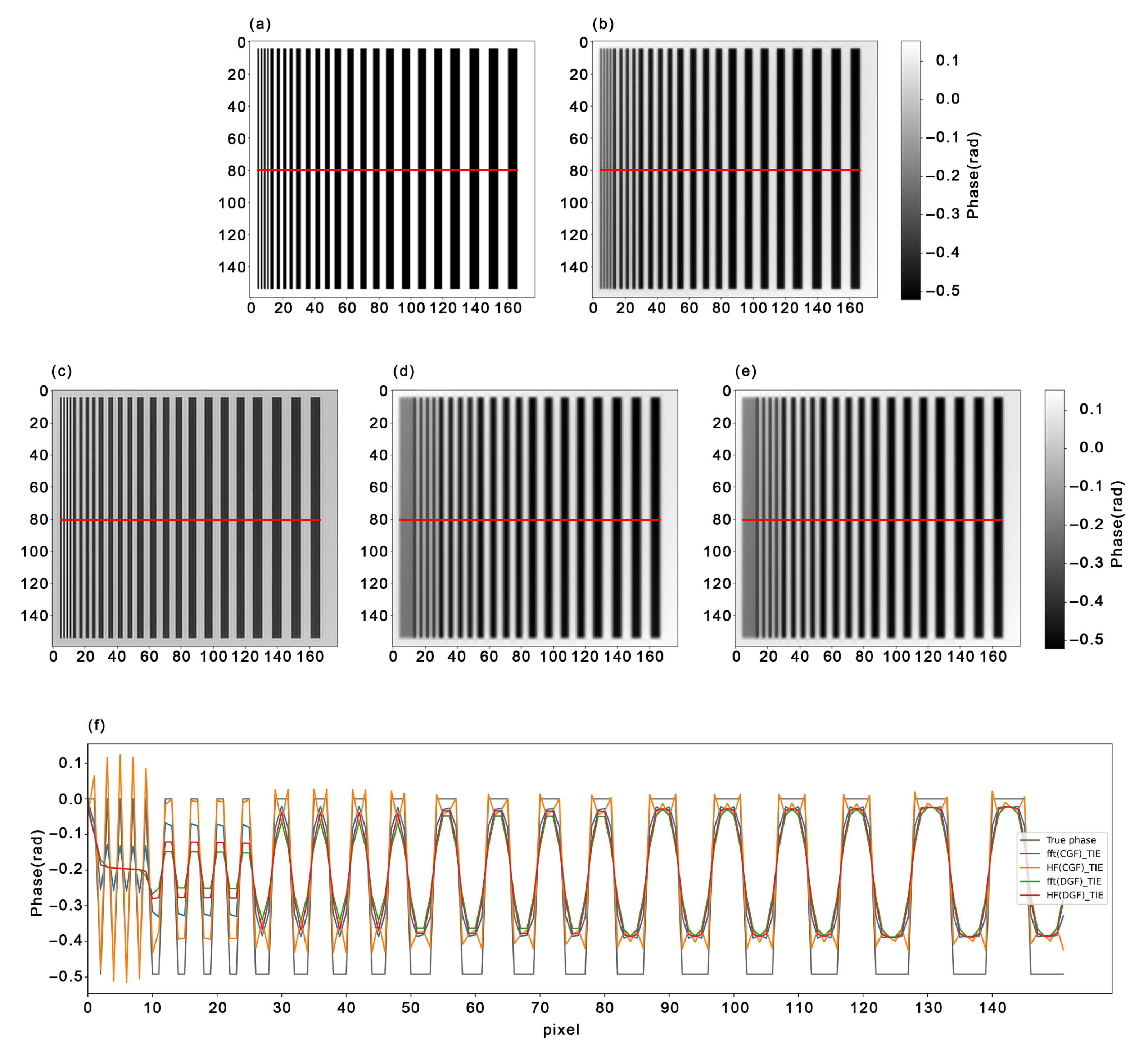
4.1. Simulated Data

As shown in Figure 2f, the pixels from 0 to 10 show the highest spatial frequency information where the phase has a period length of 2 pixel sizes. Within this range, our method HF(CGF)-TIE achieves high accuracy in the space with samples. The traditional FFT-TIE method shows a lower accuracy than our method in the space with samples, and its phase is around −0.1 radians in the space without samples. The phase fluctuates over a period length of four pixel sizes, ranging from 10 to 26 pixels. In this range, our method performs well in the space without samples. In contrast, the FFT-TIE method deviates from the true phase by approximately 0.08–0.14 radians in both the space with and without samples, with the largest difference being almost about $30\%$ of the phase shift caused by the samples. The phase in the range of 26–140 pixels has period lengths of 6, 8, and 10 pixel sizes, respectively. In this range, both our method and the FFT-TIE method achieve similar reconstruction accuracy at the full width at half maximum (FWHM) position. However, it is evident that our method exhibits more wave-like artifacts than the FFT-TIE method at the boundary between the sample and non-sample regions, and is less effective in suppressing boundary enhancement. Notably, both the FFT(DGF)-TIE and HF(DGF)-TIE methods demonstrate high insensitivity to fine structures. However, in the low-frequency spatial region, both methods yield comparable levels of reconstruction accuracy as the FFT-TIE method.

We evaluate the reconstruction quality of the phase by directly calculating the relative root mean square (RMSE) [26]:

$$RMSE={\left(\frac{\sum {\left|{\varphi }_{True}\left(\mathit{x}\right)-{\varphi }_{Rec}\left(\mathit{x}\right)\right|}^2}{\sum {\left|{\varphi }_{True}\left(\mathit{x}\right)\right|}^2}\right)}^{1/2}\times 100\%$$

(18)

where ${\varphi }_{True}\left(\mathit{x}\right)$ is the ideal image and ${\varphi }_{Rec}\left(\mathit{x}\right)$ is the reconstructed image.

The relative root mean square (RMSE) for the different approaches was 8.7% for the HF(CGF)-TIE, 14.2% for the FFT(CGF)-TIE, 23.4% for the FFT(DGF)-TIE, and 20.3% for the HF(DGF)-TIE. Our method yields a lower reconstruction error. It should be acknowledged that our approach demonstrates its superiority in the pixel range of 0–26, where the intensity fluctuations rapidly reach spatially high levels. However, in the pixel range of 26–140, our method HF(CGF)-TIE only exhibits its advantage at the boundary between the sample and non-sample regions, but also produces more wave-like artifacts. Observation of these four phase retrieval algorithms reveals that only the HF(CGF)-TIE algorithm shows significant waveform artifacts. However, these wave-like artifacts are significantly eliminated in the HF(DGF)-TIE algorithm. This suggests that the HF(CGF)-TIE algorithm is sensitive to the details of diffraction fringes produced by X-rays passing through the sample, whereas the use of DGF as a gradient operator filter removes this sensitivity but also eliminates the phase retrieval of sample details.

Based on this finding, we propose incorporating a hybrid gradient operator filter consisting of CGF and DGF into the HF(CGF)-TIE algorithm. This modification aims to strike a balance between preserving sensitivity to fine details and mitigating the excessive impact of diffraction fringes at the boundaries of the sample. We refer to this modified filter as the Modified Gradient (MG) operator filter:

$$MG=\frac{1}{2W}sin\left(2\pi W{f}_{x,p}\right)i\mathbf{i}+\frac{1}{2W}sin\left(2\pi W{f}_{y,q}\right)i\mathbf{j}+\pi f_{x,p}i\mathbf{i}+\pi f_{y,q}i\mathbf{j}$$

(19)

The explanation of the formula regarding the weights for the CGF and DGF can be found in Appendix B. We conducted a comparative analysis using the sample depicted in Figure 2a to evaluate the performance of the proposed Modified Gradient (MG) operator filter algorithm in comparison to the conventional FFT-TIE algorithm and HF(CGF)-TIE algorithm. Figure 4a,b presents the true phase and the phase reconstructed using the traditional FFT-TIE method, respectively, as shown in Figure 2a,b. Figure 4c displays the phase diagrams reconstructed using the integrated method, which combines the HF(CGF)-TIE method with the Modified Gradient (MG) operator filter. We refer to this method as HF(MG)-TIE. Additionally, Figure 4d shows line profiles across the images along the direction indicated by the lines in Figure 4a–c.

The HF(MG)-TIE method achieves a RMSE of $8.5\%$. In the pixel range of 0–10, the HF(MG)-TIE method exhibits high accuracy in the regions without samples, while simultaneously showing a phase difference of approximately 0.1 radians from the true phase in the regions with samples. In the range of 10–26 pixels, the HF(MG)-TIE method shows little variation compared to the HF(CGF)-TIE method. Notably, in the pixel range of 26–140, the wavy artifacts are significantly reduced.

We also simulated a photograph of a dog, as well as fish and leaves in Appendix A to demonstrate the generality of our approach. This picture has a nice proper high spacial frequency and low spacial frequency. To obtain the thickness of an object that ranges from 0 $\mathsf{\mu }$m to 40 $\mathsf{\mu }$m, similar to the gray-scale of the image, we divided its gray-scale by the maximum gray-scale denominator and multiplied it by 40 $\mathsf{\mu }$m. We chose an X-ray energy of 22 KeV, $\beta =3.04\times {10}^{-10}$, $\delta =7.72\times {10}^{-7}$, and a pixel size of 1.3 $\mathsf{\mu }$m (512 × 512), and we obtained the original phase map (Figure 5a) and formed a complex wave function exiting the object. We simulated a plane wave of unit amplitude which transfers through the object and propagates in free space at a distance of 0.1 m. The three phase retrieval methods have all roughly reconstructed the structure, but upon visual inspection, the gray scale of the recovered images appears lower than that of the true structure. To facilitate comparison of the numerical differences between the three methods and the true values, we plotted their profiles. As all three methods have an average phase offset of 0.5 radians higher than the true values, we subtracted a bias of 0.5 radians from the recovered values when plotting the profiles. Compared to the FFT-TIE method, the reconstructed phase variation by the HF(CGF)-TIE method fluctuates closer to the true phase, particularly in the 10–25 pixel and 30–40 pixel ranges. However, the HF(CGF)-TIE method also obtains a higher contrast than the true phase to some extent. One possible explanation for this phenomenon is that, as shown in Figure 2c, wave artifacts tend to occur in the low spatial frequency region and can spread to fine details superimposed on the native calculated value, thereby changing the contrast in fine details. The reconstructed phase obtained using the HF(MG)-TIE method showed a reduction in wave artifacts to some extent and exhibited greater accuracy compared to the FFT-TIE and HF(CGF)-TIE methods.

Table 1. RMSE of the phases reconstructed by different solutions.

Dataset	FFT-TIE Method	HF-TIE(CGF) Method	HF(MG)-TIE Method
1	14.2%	8.7%	8.5%
2	25.3%	24.6%	22.4%

presents the RMSE values for both simulation samples.

Before proceeding to the experimental part, we introduced noise in the simulated data to better align with the experimental conditions. The phases of absorption and phase-contrast images were reconstructed using different solutions, with Gaussian noise added to the images, and we refer to the noise added in [27]. The Gaussian noise with zero mean and standard deviations of 1%, 2%, 5%, 10%, and 20% of the standard deviations of the absorption and phase contrast images, respectively, was added to the absorption and phase images. The reconstructed phases were then evaluated using the root mean square error (RMSE) to quantify the accuracy of the phase retrieval.

Based on the Figure 6 and

Table 2. RMSE of phase reconstruction using different reconstruction methods when different Gaussian noise standard deviations are added independently to absorption images and phase contrast images.

Method	1% Noise	2% Noise	5% Noise	10% Noise	20% Noise
FFT-TIE	29.6%	32.5%	48.1%	62.4%	96.4%
HF(CGF)-TIE	28.8%	33.1%	48.2%	62.4%	96.4%
HF(MG)-TIE	26.7%	31.0%	47.6%	62.4%	96.3%

, it can be observed that algorithms derived from the TIE algorithm are sensitive to noise. When the noise level is low, such as 1% noise or 2% noise, our algorithm still outperforms the FFT-TIE algorithm, allowing for the retrieval of certain details. However, as the noise increases, our algorithm also exhibits haze-like artifacts, which are caused by the presence of low-frequency components in the noise [27].

The proposed approach in this study demonstrates superior accuracy in the high spatial frequency region in comparison to the FFT-TIE method. Additionally, we have employed the Modified Gradient (MG) operator filter in conjunction with our method to mitigate wave artifacts in the low spatial frequency region and achieve results that are comparable to those obtained through the FFT-TIE method in this region. When noise is introduced into the simulation, our method continues to outperform in recovering finer details when the noise level is low. However, as the noise level increases, both our method and the FFT-TIE method become susceptible to the low-frequency components of the noise, resulting in the generation of cloudy artifacts.

4.2. Experimental Data

As in the simulation case, we find from Figure 3b that not only the FFT-TIE method has low-frequency distortion, but also the HF(MG)-TIE method in Figure 3c. This phenomenon can be attributed to the requirement of having the detection of absorption maps in close proximity to the detector, resulting in a poorer signal-to-noise ratio. Consequently, larger low-frequency errors occur, leading to the observed effects. Indeed, distinguishing between the two methods with the naked eye can be challenging. However, upon closer examination of the red rectangular box area and following the arrow indications, it becomes evident that our method is capable of recovering certain transverse stripes that are not recoverable by the FFT-TIE method. Additionally, we present the phase difference between the two methods in the same region, as shown in Figure 3d, which unequivocally demonstrates that our proposed method achieves a higher level of accuracy in reproducing carbon rod fibers. Both our proposed method and the FFT-TIE method are susceptible to the low-frequency component of noise, resulting in the presence of haze-like artifacts. Despite this, our method still manages to achieve some improvement in accuracy in specific localized regions. Both our proposed method and the FFT-TIE method are susceptible to the low-frequency component of noise, resulting in the presence of haze-like artifacts. Despite this, our method still manages to achieve some improvement in accuracy in specific localized regions.

5. Conclusions

We have proposed an extension of the FFT-TIE method, which enhances the phase contrast of the reconstructed phase images of extremely fine sample features. This is achieved by employing a discrete five-point approximation scheme to estimate the inverse Laplacian. We think that the wave artifacts observed in the low spatial frequency region are caused by the sensitivity of the Continuous Gradient Operator Filter to the fine details of diffraction fringes produced by X-rays passing through the sample. To address this issue, we have combined the Continuous Gradient Operator Filter (CGF) and the Discrete Gradient Operator Filter (DGF) to form a modified Gradient Operator Filter (MG) into our proposed method. This algorithm has been effective in minimizing the impact of wave artifacts in this region and improving the overall quality of the reconstructed phase images. Indeed, experimental noise presents substantial limitations to this approach. In future studies, our plan is to incorporate noise reduction techniques to enhance the accuracy of the retrieval process while minimizing the adverse effects of noise. By implementing these techniques, we aim to further enhance the quality of the results and overcome the limitations imposed by noise. we also plan to extend this approach to datasets with higher spatial resolution. Additionally, we aim to apply this method to computed tomography (CT) imaging to accurately quantify and analyze fine feature structures.

References

1. Momose, A. Recent advances in X-ray phase imaging. Jpn. J. Appl. Phys. 2005, 44, 6355. [Google Scholar] [CrossRef]
2. Snigirev, A.; Snigireva, I.; Kohn, V.; Kuznetsov, S.; Schelokov, I. On the possibilities of X-ray phase contrast microimaging by coherent high-energy synchrotron radiation. Rev. Sci. Instrum. 1995, 66, 5486–5492. [Google Scholar] [CrossRef]
3. Mayo, S.C.; Stevenson, A.W.; Wilkins, S.W. In-line phase-contrast X-ray imaging and tomography for materials science. Materials 2012, 5, 937–965. [Google Scholar] [CrossRef] [PubMed]
4. Wang, T.; Jiang, S.; Song, P.; Wang, R.; Yang, L.; Zhang, T.; Zheng, G. Optical ptychography for biomedical imaging: Recent progress and future directions. Biomed. Opt. Express 2023, 14, 489–532. [Google Scholar] [CrossRef] [PubMed]
5. Yu, B.; Weber, L.; Pacureanu, A.; Langer, M.; Olivier, C.; Cloetens, P.; Peyrin, F. Phase retrieval in 3D X-ray magnified phase nano CT: Imaging bone tissue at the nanoscale. In Proceedings of the 2017 IEEE 14th International Symposium on Biomedical Imaging (ISBI 2017), Melbourne, Australia, 18–21 April 2017; pp. 56–59. [Google Scholar]
6. Bonse, U.; Hart, M. An X-ray interferometer. Appl. Phys. Lett. 1965, 6, 155–156. [Google Scholar] [CrossRef]
7. Förster, E.; Goetz, K.; Zaumseil, P. Double crystal diffractometry for the characterization of targets for laser fusion experiments. Krist. Tech. 1980, 15, 937–945. [Google Scholar] [CrossRef]
8. Tkachuk, A.; Duewer, F.; Cui, H.; Feser, M.; Wang, S.; Yun, W. X-ray computed tomography in Zernike phase contrast mode at 8 keV with 50-nm resolution using Cu rotating anode X-ray source. Z. Krist.-Cryst. Mater. 2007, 222, 650–655. [Google Scholar] [CrossRef]
9. Weitkamp, T.; Diaz, A.; David, C.; Pfeiffer, F.; Stampanoni, M.; Cloetens, P.; Ziegler, E. X-ray phase imaging with a grating interferometer. Opt. Express 2005, 13, 6296–6304. [Google Scholar] [CrossRef]
10. Zanette, I.; Zhou, T.; Burvall, A.; Lundström, U.; Larsson, D.H.; Zdora, M.; Thibault, P.; Pfeiffer, F.; Hertz, H.M. Speckle-based X-ray phase-contrast and dark-field imaging with a laboratory source. Phys. Rev. Lett. 2014, 112, 253903. [Google Scholar] [CrossRef]
11. Teague, M.R. Deterministic phase retrieval: A Green’s function solution. J. Opt. Soc. Am. 1983, 73, 1434–1441. [Google Scholar] [CrossRef]
12. Zuo, C.; Li, J.; Sun, J.; Fan, Y.; Zhang, J.; Lu, L.; Zhang, R.; Wang, B.; Huang, L.; Chen, Q. Transport of intensity equation: A tutorial. Opt. Lasers Eng. 2020, 135, 106187. [Google Scholar] [CrossRef]
13. Langer, M.; Cloetens, P.; Guigay, J.P.; Peyrin, F. Quantitative comparison of direct phase retrieval algorithms in in-line phase tomography. Med. Phys. 2008, 35, 4556–4566. [Google Scholar] [CrossRef] [PubMed]
14. Pogany, A.; Gao, D.; Wilkins, S.W. Contrast and resolution in imaging with a microfocus X-ray source. Rev. Sci. Instrum. 1997, 68, 2774–2782. [Google Scholar] [CrossRef]
15. Paganin, D.; Nugent, K.A. Noninterferometric phase imaging with partially coherent light. Phys. Rev. Lett. 1998, 80, 2586. [Google Scholar] [CrossRef]
16. Schmalz, J.A.; Gureyev, T.E.; Paganin, D.M.; Pavlov, K.M. Phase retrieval using radiation and matter-wave fields: Validity of Teague’s method for solution of the transport-of-intensity equation. Phys. Rev. A 2011, 84, 023808. [Google Scholar] [CrossRef]
17. Gureyev, T.; Nugent, K. Rapid quantitative phase imaging using the transport of intensity equation. Opt. Commun. 1997, 133, 339–346. [Google Scholar] [CrossRef]
18. Zhang, J.; Chen, Q.; Sun, J.; Tian, L.; Zuo, C. On a universal solution to the transport-of-intensity equation. Opt. Lett. 2020, 45, 3649–3652. [Google Scholar] [CrossRef]
19. Gureyev, T.E.; Nugent, K.A. Phase retrieval with the transport-of-intensity equation. II. Orthogonal series solution for nonuniform illumination. JOSA A 1996, 13, 1670–1682. [Google Scholar] [CrossRef]
20. Nugent, K.; Gureyev, T.; Cookson, D.; Paganin, D.; Barnea, Z. Quantitative phase imaging using hard X rays. Phys. Rev. Lett. 1996, 77, 2961. [Google Scholar] [CrossRef]
21. Tychonoff, A.N.; Arsenin, V.Y. Solution of Ill-Posed Problems; Winston & Sons: Washington, DC, USA, 1977. [Google Scholar]
22. Paganin, D.M.; Favre-Nicolin, V.; Mirone, A.; Rack, A.; Villanova, J.; Olbinado, M.P.; Fernandez, V.; da Silva, J.C.; Pelliccia, D. Boosting spatial resolution by incorporating periodic boundary conditions into single-distance hard-X-ray phase retrieval. J. Opt. 2020, 22, 115607. [Google Scholar] [CrossRef]
23. Goodman, J.W. Introduction to Fourier Optics; Roberts and Company Publishers: Greenwood Village, CO, USA, 2005. [Google Scholar]
24. Press, W.H.; Teukolsky, S.A.; Vetterling, W.T.; Flannery, B.P. Numerical Recipes 3rd Edition: The Art of Scientific Computing; Cambridge University Press: Cambridge, UK, 2007. [Google Scholar]
25. Paganin, D.; Mayo, S.C.; Gureyev, T.E.; Miller, P.R.; Wilkins, S.W. Simultaneous phase and amplitude extraction from a single defocused image of a homogeneous object. J. Microsc. 2002, 206, 33–40. [Google Scholar] [CrossRef]
26. Gureyev, T.E.; Pogany, A.; Paganin, D.M.; Wilkins, S. Linear algorithms for phase retrieval in the Fresnel region. Opt. Commun. 2004, 231, 53–70. [Google Scholar] [CrossRef]
27. Paganin, D.; Barty, A.; McMahon, P.; Nugent, K.A. Quantitative phase-amplitude microscopy. III. The effects of noise. J. Microsc. 2004, 214, 51–61. [Google Scholar] [CrossRef]
Figure 1. (a) 3D surface figure of the Fourier-space filter RMF in Equation (16) and ROF in Equation (17) plotted for the two dimensionless spatial frequencies 0 F x , F y π , where F x = 2 π W f x , p and F y = 2 π W f y , q . The RMF is visualized using the viridis color map, while the ROF is visualized using the plasma color map. (b) The one-dimensional cross sections of the RMF and ROF filters in Fourier space are visualized by setting F y = 0 or F y = π . (c) The one-dimensional cross sections of the CGF in Equation (15) and DGF in Equation (14) filters in Fourier space are visualized by setting F x = 2 π W f x , p , F y = 0 and disregarding the imaginary component.
Photonics 10 01204 g001
Figure 2. (a) Original phase, (b) phase reconstructed via the traditional FFT-TIE method, (c) phase reconstructed via HF(CGF)-TIE method, (d) phase reconstructed via the traditional FFT-TIE method, but with the CGF replaced by the DGF, is referred to as FFT(DGF)-TIE, (e) phase reconstructed via HF-TIE method, but with the CGF replaced by the DGF, referred to as HF(DGF)-TIE. (f) Line profile taken along the red line in (ae). Both the images and line profiles indicate that the HF-TIE method demonstrates higher contrast in the region of very fine sample details.
Photonics 10 01204 g002
Figure 3. (a) Phase contrast image ( I z ), (b) phase reconstructed via the traditional FFT-TIE method, (c) phase reconstructed via the HF(MG)-TIE method, and (e,f) showing enlarged images of the area highlighted by the red box in (b,c), with the yellow arrows pointing to the apparent difference between (e,f) at the same location. (d) shows the phase difference between the two methods in the region of the red box.
Photonics 10 01204 g003
Figure 4. (a) Original phase, (b) phase reconstructed via the traditional FFT-TIE method, (c) phase reconstructed via the traditional HF-TIE method, and (d) phase reconstructed using the HF-TIE method combined with the Modified Gradient (MG) operator filter. (e) Line profile taken along the red line in (ad). Both the images and line profiles indicate that the HF(MG)-TIE method demonstrates higher contrast in the region of very fine sample details and significantly reduces the wavy artifacts of the HF-TIE method.
Photonics 10 01204 g004
Figure 5. (a) Original phase, (b) phase reconstructed using the traditional FFT-TIE method, (c) phase reconstructed using the HF(CGF)-TIE method, and (d) phase reconstructed using the HF(MG)-TIE method. (e) Line profile taken along the red line in (ad).
Photonics 10 01204 g005
Figure 6. The first row of the image is an absorption map with Gaussian noise added with different standard deviations. The following lines show the phase images reconstructed with different reconstruction methods when different Gaussian noise standard deviations are added to the absorption image and the phase contrast image, respectively.
Photonics 10 01204 g006