Abstract
Addressing the inherent limitations of conventional local optimization methodologies such as damping least squares (DLS) and adaptation algorithms, this study proposes a novel approach to multi-objective optimization for imaging optical systems. The proposed method entails the formulation of a multi-objective optimization mathematical framework, where the objectives are established upon lateral aberration and wave aberration criteria. Subsequently, enhancements are made to the Non-dominated Sorting Genetic Algorithm-II (NSGA-II) by implementing a directional initial population strategy and parallel optimization with multiple-trajectory planning. The genesis of the initial population is rooted in the gradient direction information extracted from the starting positions. This strategic foundation precludes potential efficiency limitations in subsequent optimization stages arising from undesirable initial population quality. By employing mechanisms such as differentiation and mutation to sustain population diversity, the trajectory of evolution is guided by the first- and second-order derivatives of the optimal individual, thereby elevating the quality of the evolutionary offspring population. The fusion of the parent and offspring populations yields a composite population, which undergoes rapid and non-dominated sorting, crowding calculation, and elite strategies. Empirical results illustrate the validation of the proposed methodology. The proof-of-concept paradigm demonstrates high efficiency in multi-objective local optimization for imaging optical systems.
1. Introduction
In optical design, optimization constitutes a systematic endeavor to attain optimal outcomes under specified conditions. This pursuit aims to minimize the error function subject to certain constraints. Advanced, automatic optimization methods play a pivotal role in effectively and accurately determining the feasibility of achieving exemplary design results.
The current imaging optical systems are marked by increasing demands, propelled by advances in optical technology. These optical systems are expected to deliver exceptional image quality, evolving toward the large field, large aperture, and wideband to meet the diverse demands. Moreover, optical systems have grown increasingly complex, transitioning from coaxial and off-axis configurations to partial-axis ones, and from spherical and aspheric surfaces to freeform surfaces. Consequently, the task of seeking the increasingly untraceable initial structure of optical systems, whether in existing systems or patent libraries, has become infeasible.
Complex optical systems inherently involve a multitude of structural parameters for optimization, comprising continuous and discrete variables. Aberrations manifest as nonlinear functions of these variables, impeding the derivation of analytical expressions. Additionally, aberrations are asymmetric in an optical system with freeform surfaces [1,2,3]. The types of aberrations are also increasing and lack orthogonal relationships, resulting in a number of local minima within the multidimensional variable space, rendering the quest for optimal solutions in imaging optical systems a hard effort. Commercial optical design software, like CODE V and Zemax, predominantly employs the DLS method for automated local optimization of imaging optical systems, focusing on one specific objective, such as RMS spot, wave aberration, or MTF. Alternatively, users can achieve optimization by constructing complex error functions, such as combining lateral aberration with wavefront aberration to form a complex error function, and then performing optimization. However, this approach transforms multiple objectives into a single objective, which achieves the optimization process through a single objective algorithm, essentially. As a result, recent research in imaging optical systems has concentrated on single-objective optimization [4,5,6]. However, conventional single-objective local optimization methodologies, such as DLS and adaptive methods, may prove inadequate for complex optical system types that necessitate the simultaneous optimization of multiple targets.
Numerous multi-objective optimization algorithms have been proposed to solve problems that single-objective optimization algorithms cannot overcome. David Goldberg proposed a multi-objective optimization technique named genetic algorithm (GA) [7]. Subsequently, Srinivas and Deb devised NSGA, grounded in the concept of non-dominated sorting [8]. Deb et al. enhanced NSGA with NSGA-II [9], which adopts the congestion and crowding comparison operator as the winning criterion in peer comparison after fast sorting and maintaining the diversity of populations. The proposed method also introduces the elitist strategy, enlarges the sample space, prevents the loss of the best individual, and improves the computing speed and robustness of the algorithm. The algorithm is highly suitable for processing multi-objective optimization problems with ≤3 objective dimensions. R Furtuna et al. designed a method based on NSGA-II to improve the multi-objective optimization problem in the chemical synthesis process. However, the application is not universal as it requires high parametric conditions during chemical reactions [10]. Hossein et al. proposed an enhanced version of NSGA-II to solve the fuzzy bi-objective assembly line balancing problem, where the objective function is to minimize the number of workstations and the fuzzy cycle time [11]. Khettabi et al. first proposed a reconfigurable manufacturing system for cost, time efficiency, and environmental awareness. Adaptive dynamic NSGA-II and NSGA-III were developed for this system [12].
The objective optimization algorithms mentioned above are all based on genetic algorithms. Nevertheless, these algorithms remain somewhat specialized, being tailored to specific multi-objective problems such as allocation [13,14,15], vehicle routing [16,17,18], the traveling salesman problem [19], and scheduling dilemmas [20,21,22]. Their universal applicability is limited because a generic problem-solving approach may not surpass a technique specifically tailored to the given problem. The precision and efficiency of these algorithms would not meet the application requirements in the complex operating environment of the target to be optimized, such as the multi-objective optimization of imaging optical systems. Therefore, this paper makes improvements to the traditional NSGA-II multi-objective optimization algorithm to make it suitable for optimizing imaging optical systems.
This paper investigates the use of the multi-objective local optimization method—an algorithm that does not require transforming multiple objectives into one—with optical systems. It can directly optimize multiple objectives simultaneously and provide a non-dominated solution set as the output. This solution set allows designers to find the optimal solution according to their optimization target and strategy. This approach significantly improves the efficiency of optical design and the quality of design results, which has both theoretical significance and practical value for developing optical optimization technology.
2. Methods
2.1. Mathematical Model of Multi-Objective Optimization
Optimizing optical systems involves minimizing error functions in the multidimensional nonlinear space of structural parameters. The error function of an optical system reflects the imaging quality of the system and is a complex nonlinear function associated with structural parameters. Considering the requirements for system design—including focal length, magnification, image distance, and exit pupil position—the error function is subject to constraints that can be mathematically expressed as linear and nonlinear equations related to the structural parameters of the system.
Traditional optimization for optical systems usually adopts single-objective optimization methods, such as the DLS and adaptation methods. The mathematical model is shown in Equation (1).
where Φ(X) is the objective error function; g(X) is the inequality constraint; h(X) is the equality constraint; and X = [x1, x2, x3, …, xn] are variables of the optical system.
Facing various requirements of the upcoming design, the multi-objectives, usually featuring trade-offs, should simultaneously be minimized to a desirable level. However, even if one error function has fallen into the required level, it poses a challenge to achieve the simultaneous decline of multiple objectives. For instance, commercial imaging optical software—such as CODE V and Zemax—can effectively optimize the system when combined with one error function, including lateral aberration, wavefront aberration, and MTF, all of which can reflect the imaging quality of the optical system from different perspectives. However, the single-objective optimization process based on such software cannot guarantee other error function reduction. Here, the mathematical model of the multi-objective framework is listed in Equation (2).
where Φ1(X) and Φ2(X) are the error functions; g(X) is the inequality constraint; h(X) is the equality constraint; and X = [x1, x2, x3, …. xn] are variables of the optical system.
In essence, multi-objectives need to be optimized simultaneously for optical systems that pursue the ultimate performance of these aberrations. In this study, we constructed a double objective error function associated with lateral and wave aberration for this purpose.
The lateral aberration error function represents a center-weighted RMS spot size, where the function is calculated by ray tracing through the ray grid of each weighted wavelength and field. As the sum of squares of the aberration function, the structure of the function is conducive to the convergence of subsequent models [23]. The calculation for the lateral aberration error function is shown in Equation (3).
where Φ1 is the lateral aberration error function; WF is the weight of field; Wλ is the weight of wavelength; Δη and Δδ are lateral aberrations of meridian and sagittal directions; WR is the weight of the aperture’s position; fi is the sum of aberrations for each field and wavelength; and M is the product of the number of fields and working wavelength.
Specifically, lateral aberration is calculated by tracing the rays of sampling points for each field and wavelength to obtain the x and y coordinate values of each ray at the image plane. The coordinate value pertaining to the principal ray on the image plane from the previously acquired coordinate value is to be subtracted. The lateral aberration Δx and Δy can be obtained in the x and y directions.
The weight of the aperture represents the proportion of light rays with different apertures. The weight increases as the aperture position of the light decreases. The weight of the aperture can be calculated using Equation (4).
where WR is the weight of the aperture, and (ρx, ρY) represents the coordinates of the light rays in the pupil.
The wavefront aberration error function is used for characterizing the difference between the actual wavefront and the ideal wavefront. Here, the optical path difference is calculated by tracing the sampled rays at each wavelength and field, and
where Φ2 is the wavefront aberration error function; WF is the weight of field; Wλ is the weight of wavelength; WR is the weight of aperture position; and opd is the optical path difference.
2.2. Method Design
2.2.1. Establishment of Directional Initial Population
Initializing the population is the first step in optimization methods and serves as the foundation of the overall strategy. Optimizing the initial population can improve subsequent convergence efficiency. In the population initialization stage, the traditional strategy usually adopts random steps to construct the initial population, which has a relatively high possibility of causing a deterioration in the imaging quality of the optical system because the solution may fall into a local optimum. Meanwhile, the strategy would initially form many infeasible schemes, thereby reducing the computational efficiency of the algorithm. This study proposes establishing an initial population based on the gradient direction information in order to address this issue. This approach helps to avoid the problem of low-quality initial populations, leading to improved efficiency in subsequent optimization.
First, the improved Levenberg–Marquardt (LM) method [24] is adopted to confirm the initial population direction. According to the initial variables and error function information, the second-order Taylor expansion [25] approximates the error function Φ1 at xk, as shown in Equation (6).
where error functions are characterized by vectors f = [f1, f2, … fN]; J(xk) is the Jacobi matrix of f(xk) at xk; and ∇2 fi(xk) is the Hessian matrix of f(xk) at xk.
By taking the derivative of Equation (6), Equation (7) can be obtained as follows:
where f is the error function vector matrix for each field and each band; J is the Jacobi matrix of f; H is the Hessian matrix of f; and d is the step for variable changes, which causes the error function to decrease.
The initial population is established based on the descending direction, d, as shown in Equation (8).
where v0 is the initial variable vector; vi is the i-th value of the initial population, i ∈ (1, M); M is the total number of populations; and d is the step calculated by Equation (7).
As a result, an initial population is established along the determined direction, providing a reliable initial guess for the subsequent evolution process. This approach can effectively accelerate population convergence and improve the accuracy of solutions.
2.2.2. Multi-Trajectory Parallel Evolution
The evolution operation is the core step of optimization algorithms based on GA, which directly inherits excellent individuals to the next generation through selection, or generates new individuals through pairing, crossover, and mutation. This step determines the quality of the offspring population. The traditional NSGA-II algorithm often generates offspring through tournament selection algorithms. Binary tournaments involve extracting two individuals from the population at once, selecting the optimal individual from the pair, and placing it into the next generation population. This selection mechanism is unsuitable for specific multi-objective problems since it lacks a clear evolutionary direction, making it challenging to drive the optical system to a desirable optimal level. To address this issue, this paper further proposes a multi-trajectory parallel optimization strategy to improve the quality of the offspring population and ensure diversity through various means.
The evolutionary process for offspring generation is divided into two strategies—the LM strategy and the differential strategy. The LM strategy is adopted in order to improve the quality of the offspring population, and the differential strategy is used to enhance the diversity of the offspring population.
For the LM strategy, the individual with the best quality in the parent generation is selected as the reference point in each offspring evolution process, and its descent direction is calculated as the evolution direction. During evolution, 50% of the parent generation’s population is added to the step length in the descending direction to achieve evolution.
For the differential strategy, a particular offspring evolution mechanism is achieved by randomly selecting three individuals from the parent population and differentiating two of them. The differentiated results are then combined with other individuals by setting a scaling factor and a particular mutation rate to obtain new offspring individuals.
where v0i is the i-th initial variables; vi is the i-th variables of the offspring population; v1i, v2i, and v3i are the i-th variable of three individuals randomly selected from the parent population, respectively; F is the scaling factor; and R is the mutation rate.
The offspring population obtained through differential strategy evolution accounts for 50% of the total population. Therefore, for the parent population with a quantity of M, one half of the offspring population is evolved through the LM strategy, and the other half is evolved through the differential strategy. The parent and offspring populations are then merged into a population of 2M, and the best M individuals are selected to enter the next generation population.
2.2.3. Method Process
This paper proposes a multi-objective optimization method for imaging optical systems by improving NSGA-II. The schematic diagram of the proposed multi-objective optimization method is shown in Figure 1. In Figure 1, L1 … Lm represents non-dominated levels; LC1 … LCn represents population individuals within the same non-dominated level, in descending order of crowding; Pt represents the original population; and Pt+1 represents a new population after evolution for one generation. Specifically, the initial population is established based on the gradient direction information of the optimized initial value, which helps in avoiding low efficiency in subsequent optimization due to poor initial population quality. Additionally, multi-trajectory parallel evolution is made to enhance the quality and diversity of the offspring population.
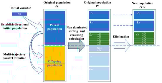
Figure 1.
Schematic diagram of the proposed multi-objective optimization method.
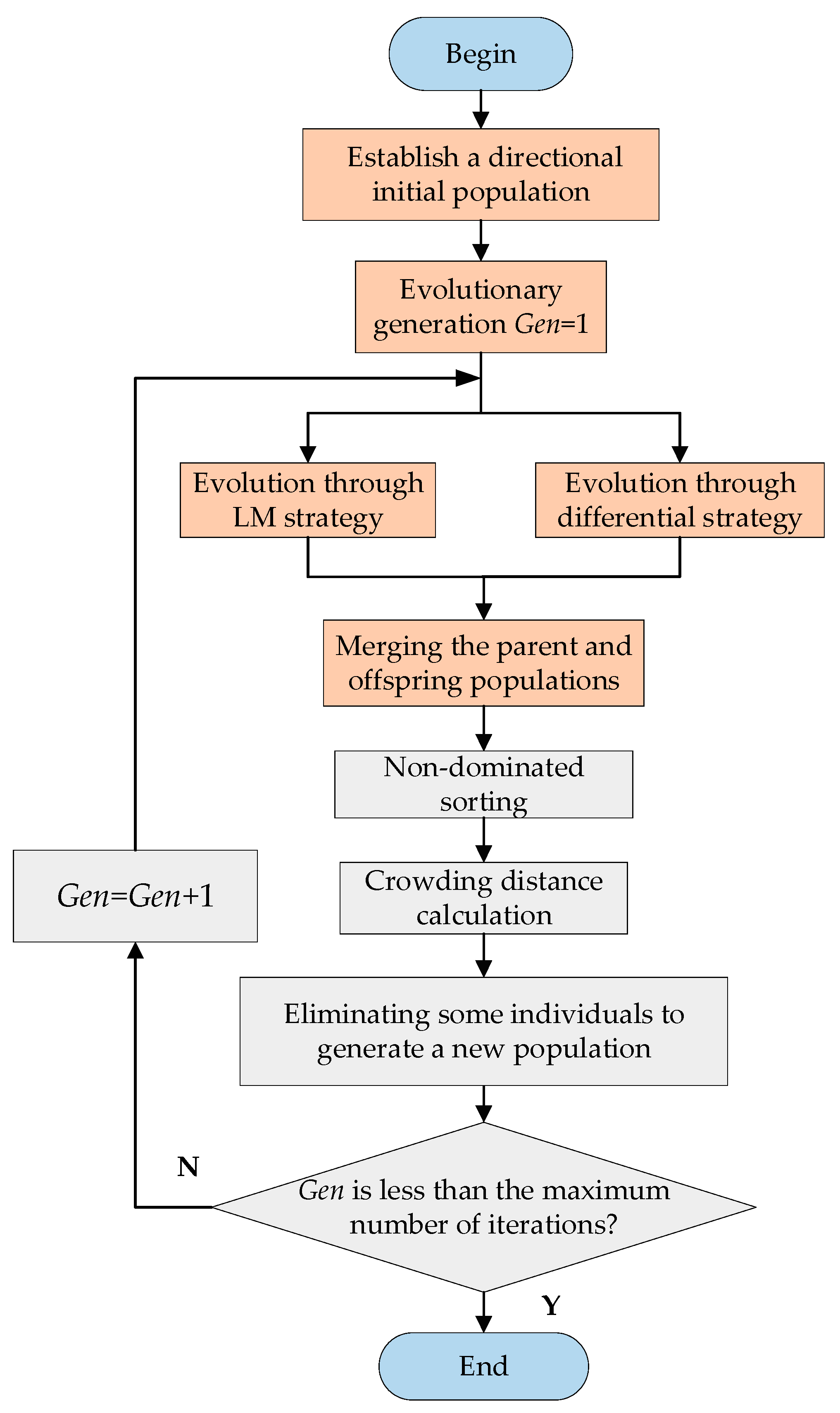
The algorithmic process is depicted in Figure 2. Initially, a population comprising M individuals is established based on predefined error functions and gradient information pertaining to the initial variables. The computational procedure can be referenced via Equations (7) and (8). The generation of offspring is accomplished through the crossing of parent individuals, resulting in N offspring. After setting the crossover probability CR, the offspring population quantity N is the product of the parent population quantity M and the crossover probability, i.e., N = M × CR. Subsequently, the evolutionary process is divided into two parallel strategies. Half of the N offspring populations undergo evolution using the LM strategy, while the remaining half evolve through the differential strategy. Consequently, N offspring populations are generated by employing the parallel evolutionary approaches. In the next phase, the parent and offspring populations are amalgamated to form a new population consisting of (M + N) individuals. The population level is established and individuals are sorted within the level through non-dominated sorting and crowding calculation. The elimination operation is performed, retaining only the first M individuals to update the population. The iteration termination condition is evaluated by reaching the maximum number of iterations.

Figure 2.
Flow chart of the proposed multi-objective optimization method.
3. Experiments and Results
To evaluate the validation of the proposed method, two sets of multi-objective optimization experiments are conducted using a Cooke optical system (Case 1) and a self-developed telescope system (Case 2). In Case 1, the system has been optimized for spot size using commercial software CODE V (version: CODE V 11.5), which is a minor aberration system, as shown in Figure 3. For Case 2, the image quality has not been optimized, which has a relatively large aberration compared with Case 1, as shown in Figure 4. Double objective optimization upon lateral and wave aberration error functions is performed. The variables of the system are labeled in Figure 3 and Figure 4, including curvatures and thicknesses, respectively marked with “C” and “d”. The multi-objective error function and optimization program is coded by Matlab R2017a, and the ray tracing of CODE V software is invoked to achieve the optimization iteration process. The number of individuals in the initial population, M, is set as 50; the number of offspring population, N, is 30; the scaling factor, F, is set as 0.5; and 0.5 of the variation rate (R) is adopted in Equation (9).
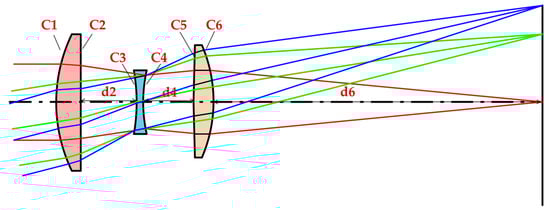
Figure 3.
Cooke optical system (Case 1).
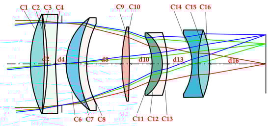
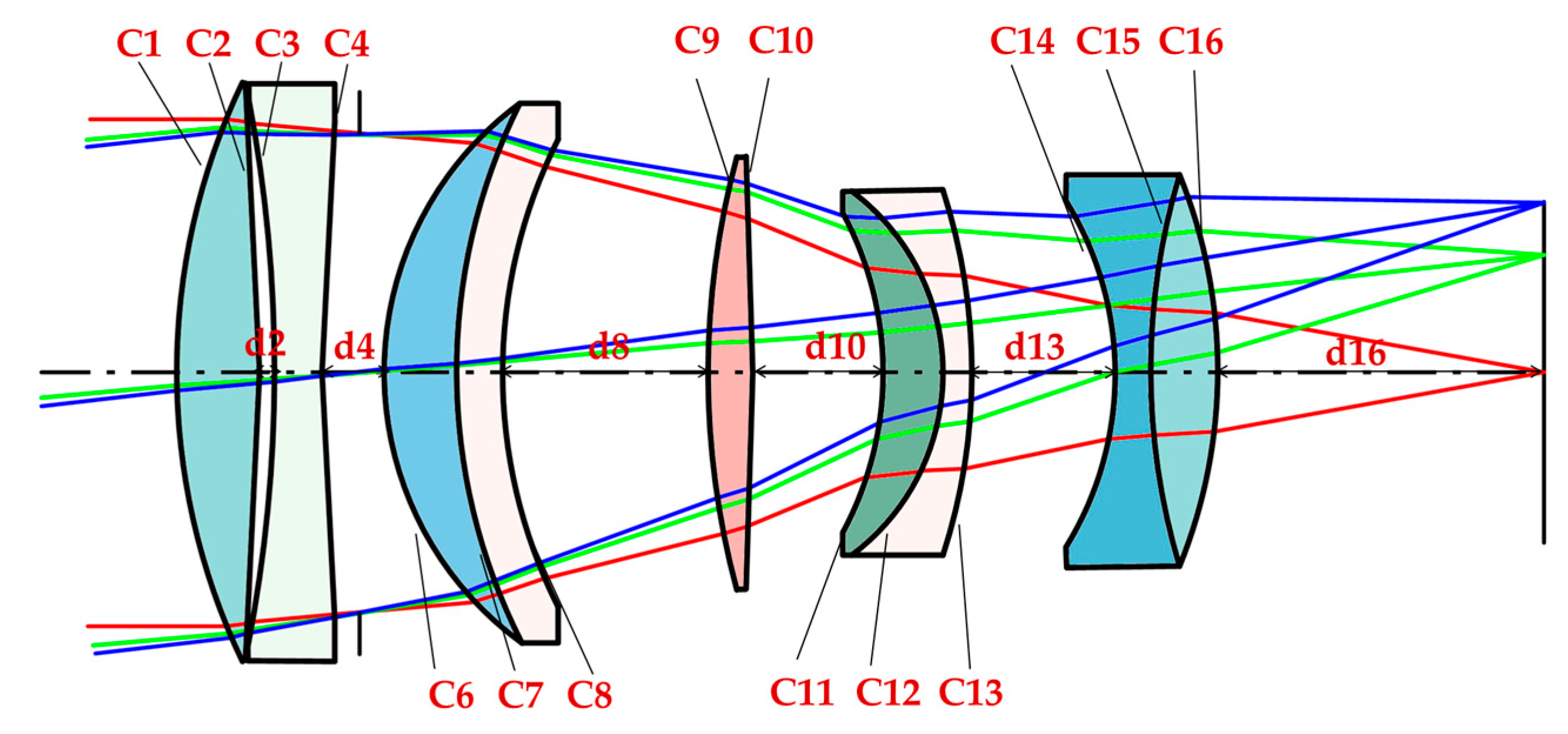
Figure 4.
Self-developed telescope system (Case 2).
Table 1 shows the basic parameters of the optical systems used in the two cases. A single wavelength for both lenses is employed to simplify the experimental parameters and exclude the influence of chromatic aberration factors, such as the secondary spectrum. These parameters were carefully selected to ensure accurate and reliable experimental results.

Table 1.
Basic parameters of the optical systems used in two cases.
3.1. Experiment with the Cooke System
The initial parameters and variables of the Cooke optical system are shown in Table 2. We have set nine variables in this system, labeled with “v” in the table. Through calculation, the lateral aberration error function of this system is 18.236, and the wavefront aberration error function is 1.435. We attempted to increase the thickness of surface 4 and the curvature of surface 1 of the Cooke system, in order to characterize the mapping relationship between the optical system variables and the error function. Then, the lateral aberration error function and wavefront aberration error function under the corresponding optical system parameters are calculated.
Table 2.
Initial parameters and variables of Case 1.
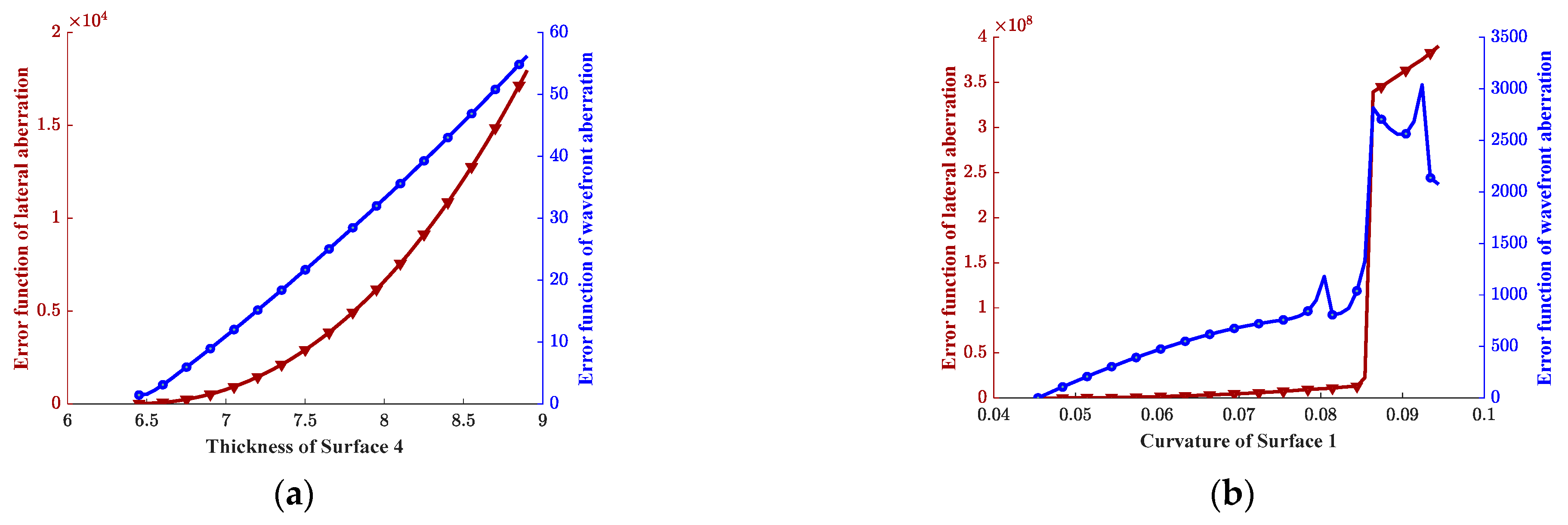
Figure 5 shows the relationships between the variation of the double objective and both the thickness of surface 4 and the curvature of surface 1. These results provide insights into the impact of optical system variables on error functions and a hint for guiding the optimization process. As shown in Figure 5a, the lateral aberration and wavefront aberration error functions exhibit a similar increasing trend with the thickness of surface 4 in the interval from 6.5 to 9. However, for the curvature variable, as shown in Figure 5b, the trends of the two error functions are consistent in the interval of curvature from 0.05 to 0.08. In contrast, in the interval of curvature from 0.08 to 0.082 and from 0.086 to 0.009, the wavefront aberration error function decreases while the lateral aberration error function increases. These results suggest that the trends of the lateral aberration and wavefront aberration error functions are generally consistent. However, there are also situations where their trends are contradictory. It should be noted that the thickness of surface 4 and the curvature of surface 1 are randomly chosen. We can obtain similar conclusions by modifying the variables to other surfaces and performing this process again.
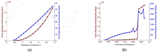
Figure 5.
Mapping the relationship of the double objective function with respect to the variables. (a) Trend of the double objective function with thickness of surface 4; (b) Trend of the double objective function with curvature of surface 1.
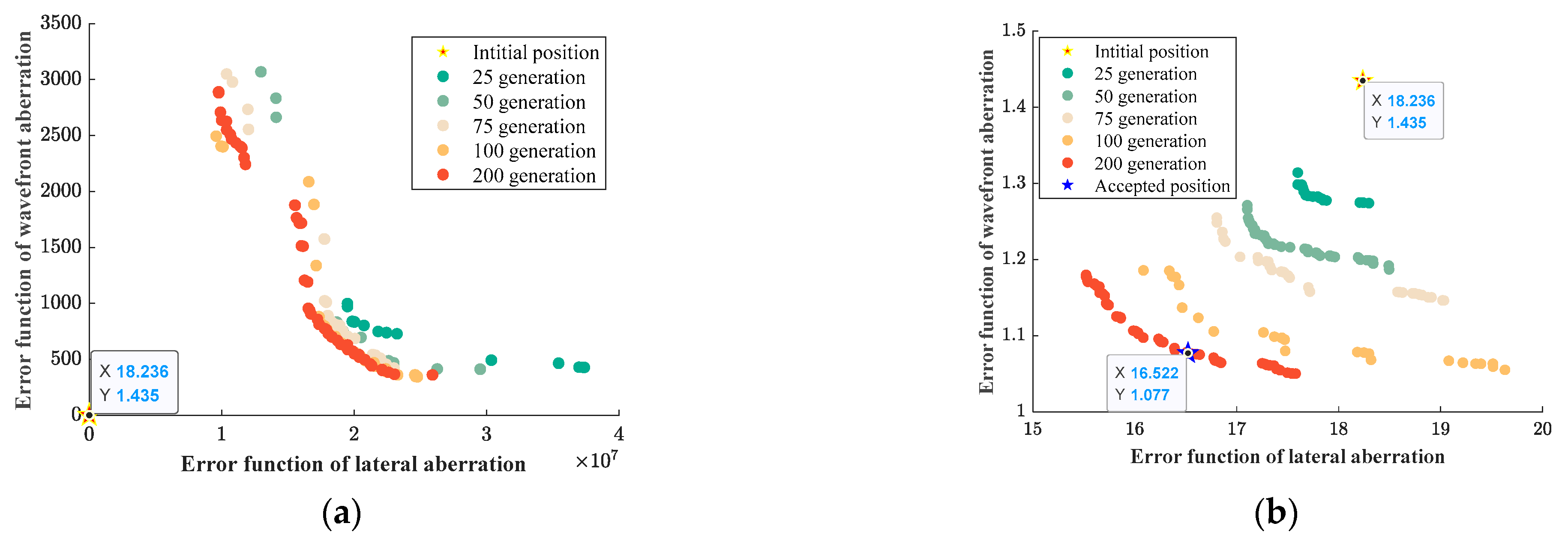
Since the image quality of this system has already reached a better standard than the initial state, it is easy to deteriorate the originally better image quality again if the initial population is established by randomly adding step length with this initial variable into the 9-dimensional variable space. By using the proposed method of establishing a directional initial population, we calculated the direction vector s = [5.591 × 10⁻⁷, −1.706 × 10⁻⁷, −1.002 × 10⁻⁸, −5.435 × 10⁻⁸, −2.238 × 10⁻⁷, 2.702 × 10⁻⁷, 0.0005946, −0.001302, 0.001457], which refers to the direction of evolution when establishing the population. The variables in Table 2 were used as initial values, while the direction vector s was used as the step length to create an initial population with a number of 50 by Equation (8). Figure 6 shows the Pareto fronts for different evolutionary stages. The initial position and Pareto front for evolutionary generations 25, 50, 75, 100, and 200 are also labeled in the figure. Since this is a multi-objective analysis, the final result is not unique, but a set of non-dominated solutions, and the final optimal solution can be selected from the solution set according to the design needs.

Figure 6.
Optimization results of different algorithms. (a) Pareto front for the evolutionary process of NSGA-II; (b) Pareto front for the evolutionary process of the proposed multi-objective optimization method.
As shown in Figure 6, the proposed multi-objective optimization method achieves much better double-objective function reduction compared to the original NSGA-II algorithm for the same number of evolutionary generations. Figure 6a shows that the optimized results of the original NSGA-II algorithm are worse than they were in the initial position. In contrast, the Pareto fronts of the proposed method continue converging to the lower left as the number of evolutionary generations increases, and the optimization results continue to improve with respect to the initial results. Although CODE V has previously optimized the Cooke optical system, our proposed method further improves its performance. Optimization results of 200 generations are selected as the final Pareto solution set. If we choose a lateral aberration error function value of 16.522 in this solution set as an acceptable position, the wavefront aberration error function is 1.077. The initial and optimized variables and error functions of the Cooke system are shown in Table 3. After this optimization, there is a reduction of 12.26% in the lateral aberration error function and 24.94% in the wavefront aberration error function. It should be noted that our criterion for selecting acceptable positions is the desire to have an effective balance between the lateral aberration error function and the wavefront aberration error function values. In practical applications, designers can define the judgement criteria of acceptable positions according to the design needs of different optical systems.
Table 3.
Initial and optimized variables and error functions of Case 1.
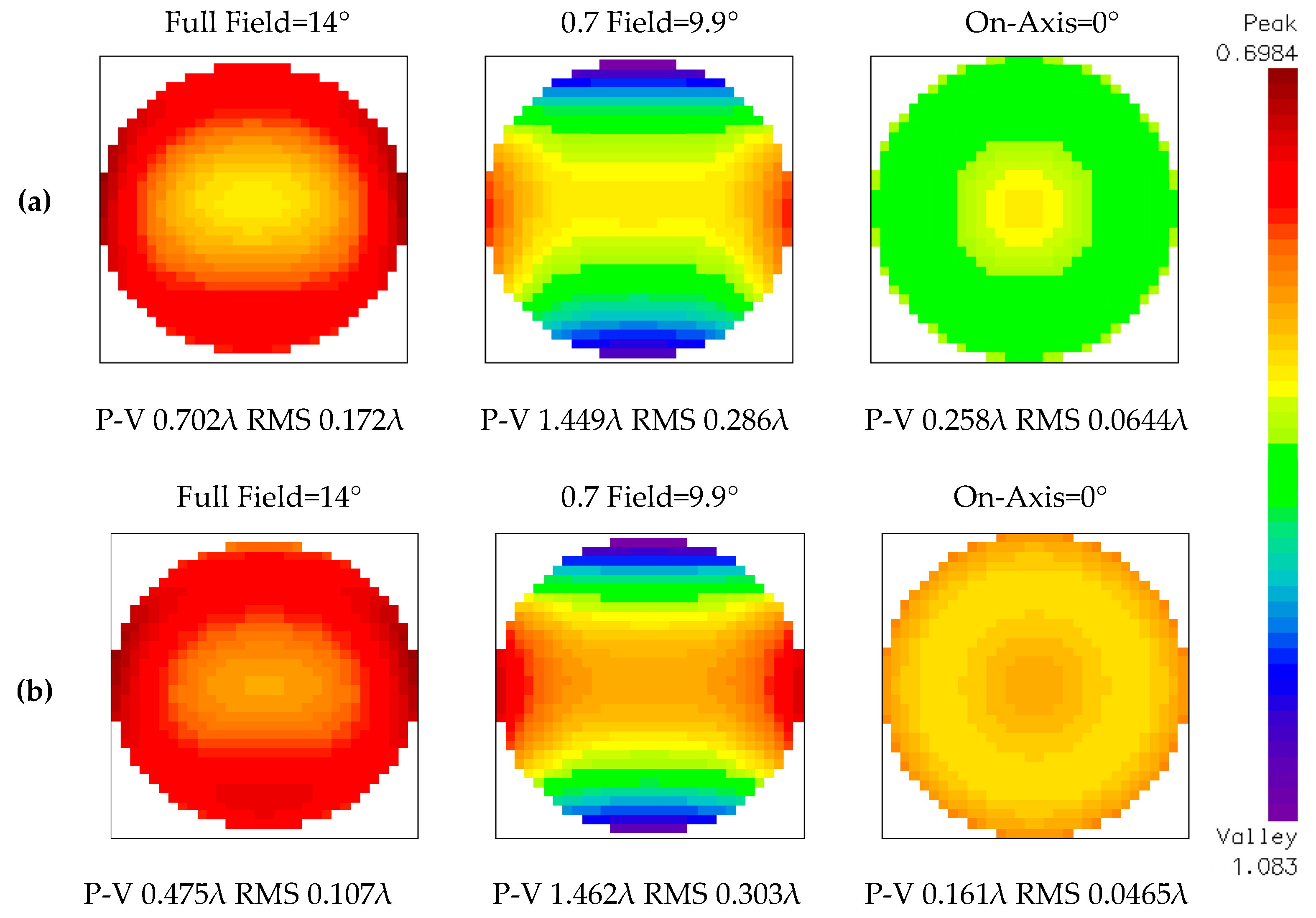
Figure 7 shows the comparison of wavefront aberration before and after optimization, with RMS values of 0.0644λ, 0.286λ, and 0.172λ for the three fields of the system before optimization. After optimization, the RMS values of the three fields of the system are: 0.0465λ, 0.303λ, and 0.107λ. Although the wavefront aberration of the second field has slightly increased compared to before optimization, the overall wavefront aberration value of the entire system has improved. These results demonstrate that the proposed method effectively converges the error function of the minor aberration system, resulting in a significant enhancement of image quality.

Figure 7.
Comparison of image quality before and after optimization. (a) Wave aberration before optimization; (b) wave aberration after optimization.
3.2. Experiment of the Self-Developed Telescope System
The image quality of the self-developed telescope system has not been optimized previously. The initial image quality is poor due to its large aberration. The number of variables in this system is 21, and the variables are labeled with “v” in the table. The initial parameters of this telescope system are shown in Table 4.
Table 4.
Initial parameters and variables of Case 2.
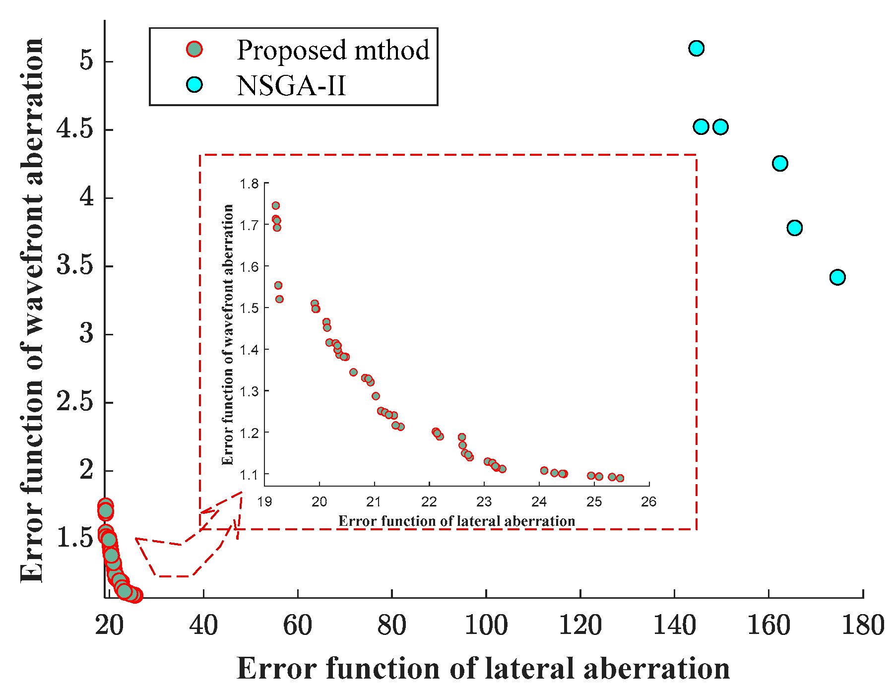
Figure 8 shows the Pareto front curve after 200 generations of optimization using the proposed multi-objective optimization method and NSGA-II. The results demonstrate that this algorithm optimized the telescope system more effectively compared to NSGA-II. Utilizing the proposed algorithm, both the lateral aberration and wavefront aberration were greatly improved as a result of the optimization. If we choose a lateral aberration error function value of 19.230 as an acceptable position, the final wavefront aberration is 1.709.
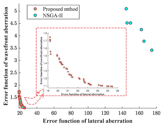
Figure 8.
Optimization results of the proposed multi-objective optimization method compared with NSGA-II.
Comparisons of variable values and error functions before and after optimization are shown in Table 5. The initial lateral aberration error function was 20,957.51, and the initial wavefront aberration error function was 106.24 before optimization. After optimization, the values of the double objective functions were reduced to 19.230 and 1.709, respectively. These results demonstrate a significant reduction in error functions by about two to three orders of magnitude compared to the initial state. The results highlight the effectiveness of our proposed method for optimizing large aberration systems.
Table 5.
Initial and optimized variables and error functions of Case 2.
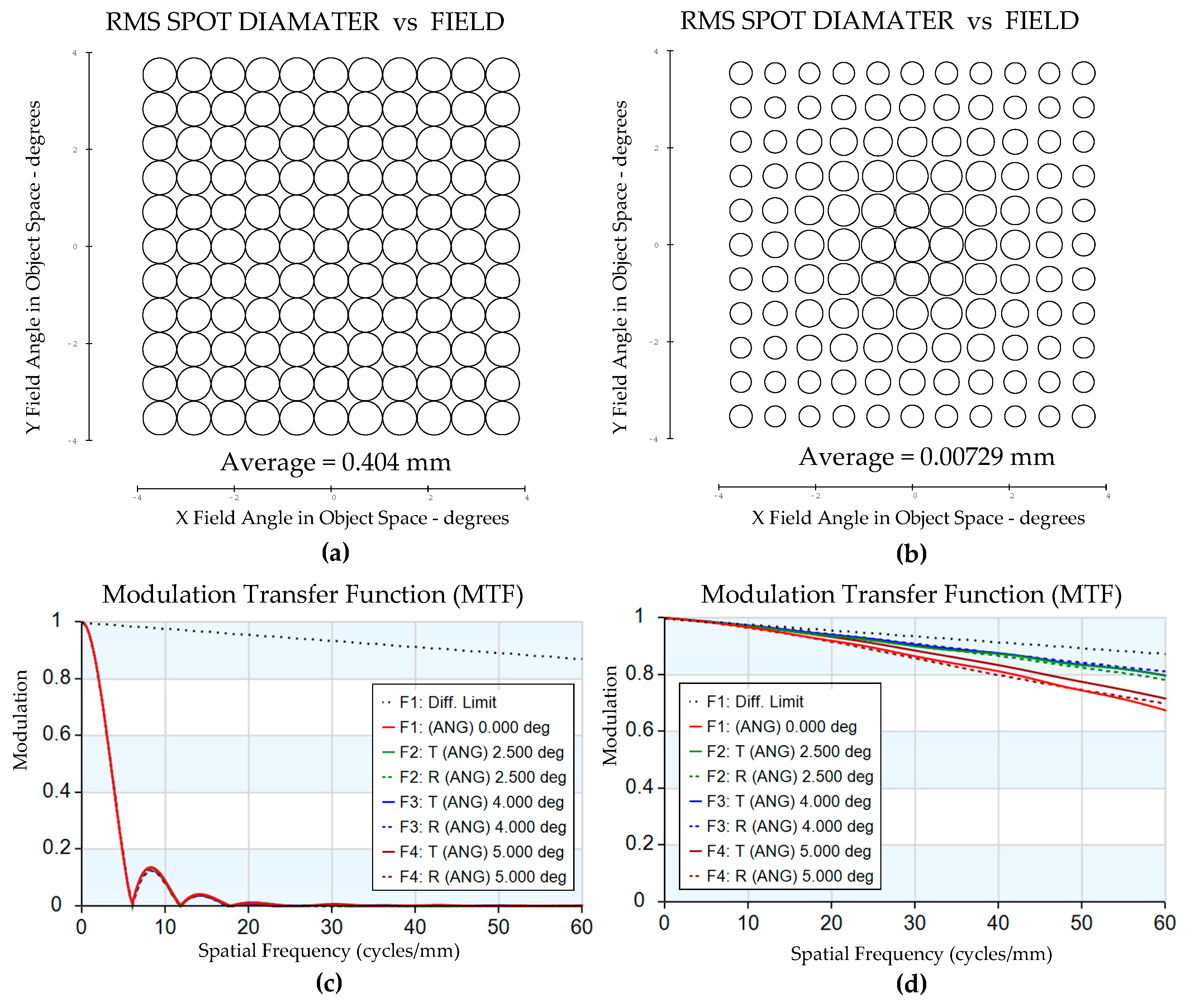
A comparison of the RMS geometry spot and MTF before and after optimization is shown in Figure 9. Before optimization, the average RMS spot diameter of the optical system was 0.404 mm. After optimization, this value was significantly reduced to 0.00729 mm. Additionally, the MTF at the feature frequency of 60 lp/mm was less than 0.1 before optimization, but increased to more than 0.6 for the full field after optimization. These results demonstrate that the proposed method effectively converges the error function of the large aberration system, resulting in significant improvements in image quality.
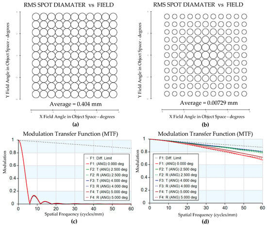
Figure 9.
Comparison of image quality before and after optimization. (a) RMS spot field map before optimization; (b) RMS spot field map after optimization; (c) MTF before optimization; (d) MTF after optimization.
The above experiments have revealed that the method proposed can optimize two objective functions simultaneously. To further demonstrate the applicability of the proposed method, we constructed the third error function based on distortion in this section. Among them, Objective 1 is the lateral aberration error function, and Objective 2 is the wave aberration error function. The construction of these two error functions has been described in Section 2.2.1. Target 3 is the error function based on distortion, which represents the deformation between the actual image plane and the ideal image plane after imaging by an optical system. The calculation for the error function based on distortion is shown in Equation (10).
where Φ3 represents the error function based on distortion, L’ is the paraxial image height, and L’p is the main ray image height in the current field.
The test cases and optimization variables in three objective optimization experiments are consistent with those of the dual objective experiment, and the number of individuals in the initial population and offspring population parameters are also consistent with those of the dual objective experiment. The Cooke system (Case 1) and the self-developed telescopic system (Case 2) have been optimized for 200 generations using the proposed method. Comparisons of three error functions before and after optimization are shown in Table 6. The results demonstrate that this algorithm optimized three error functions for the Cooke and telescope system effectively. For Case 1, if we choose a lateral aberration error function value of 18.19 as an acceptable position, the final wavefront aberration error function value is 1.41 and the distortion error function value is 0.0266. Compared with the initial value, the lateral aberration, wavefront aberration, and distortion were greatly improved after optimization. For the large aberration system, Case 2, the proposed algorithm has also improved the three objectives, ultimately achieving ideal image quality for the large aberration optical system.
Table 6.
Comparison of three error functions before and after optimization.
4. Discussion
Simulation experiments are conducted to demonstrate the effectiveness and reliability of the proposed multi-objective local optimization method. Firstly, error functions based on lateral and wavefront aberrations are established, and the mapping relationship between the two error functions and variables is analyzed. The results show that the variation trend of lateral and wavefront aberration error functions with the same variable is not always consistent. Sometimes, the lateral aberration and wavefront aberration trends are contradictory. Subsequently, two sets of multi-objective optimization experiments were conducted using small and large aberration systems, respectively. For the small aberration system (Case 1), although the image quality of the system has been optimized previously, the proposed method can still further improve it. For the large aberration system (Case 2), the lateral and wavefront aberrations of the system have been greatly improved after optimization, and the Prato front solution set is provided as output. By taking one set of acceptable values as the final result, the average RMS spot diameter of the optical system before optimization is 0.404 mm, and the value after optimization is 0.00729 mm. The MTF at the feature frequency of 60 lp/mm before optimization is less than 0.1, and the value after optimization is higher than 0.6. Therefore, this method has excellent universality for small and large aberration optical systems. For time efficiency, the implementation process of this algorithm mainly takes up two periods of time: one is the time for invoking CODE V from Matlab, and the other is the running time for the optimization algorithm in Matlab. The running time of pure optimization algorithms is much lower than that of invoking CODE V from Matlab, and the data transfer between software interfaces takes up a lot of time. Taking self-developed telescope systems for example, when iterating for 25 generations, the optimization algorithm time is 3.2 s, while the time for invoking CODE V from Matlab is 163.7 s, which takes up 98.08% of the total program running time. If only one type of software is used for achieving the entire optimization process, the optimization efficiency will be greatly improved. It should be further noted that since the method made enhancements to NSGA-II, non-dominated sorting and crowding calculation operations are still preserved. Therefore, this proposed method is more suitable for situations where the number of optimization objectives is ≤3. In addition, the proposed method is currently applicable to unconstrained multi-objective optimization for imaging optical systems, and methods based on penalty function or searching for feasible solutions can be employed to handle cases with constraints. However, by effectively improving the performance of optical systems, the proposed method can contribute to the development of high-quality optical systems for a range of applications. Meanwhile, the idea of directional calculation of initial population and multi-trajectory parallel evolution proposed in this study has a certain reference value in other multi-objective optimization algorithms based on search or evolution.
5. Conclusions
In order to address the inherent limitations of conventional local optimization methodologies, such as DLS and adaptation algorithms, we have proposed a multi-objective optimization method suitable for imaging optical systems, where the objectives are established upon lateral aberration, wave aberration, and distortion criteria. Subsequently, enhancements were made to the NSGA-II algorithm by implementing a directional initial population strategy and parallel optimization with multiple-trajectory planning. These enhancements help to identify the direction of evolution and ensure the diversity of the population. The parent and offspring populations are merged into a new population, and fast and non-dominated sorting, crowding calculation, and elite strategy are performed on the population. Experimental results demonstrate the effectiveness of the proposed method. With the initial parameters optimized by CODE V, our method further reduces the lateral and wavefront aberration error functions of the Cooke system by 12.26% and 24.94%, respectively. For the self-developed telescope system, the average RMS spot diameter of the optical system before optimization is 0.404 mm, and the value after optimization is 0.00729 mm. The MTF at the feature frequency of 60 lp/mm before optimization is less than 0.1, and the value after optimization is higher than 0.6. This study provides essential guidance for applying multi-objective optimization in imaging optical systems, and contributes to the development of high-quality optical systems for a range of applications.
Author Contributions
Conceptualization, S.Z.; methodology, S.Z. and H.W.; software, S.Z. and H.Y.; validation, S.Z. and J.H.; formal analysis, S.Z.; investigation, M.H.; resources, X.Z.; data curation, H.Y.; writing—original draft preparation, S.Z. and J.H.; visualization, H.Y.; supervision, X.Z.; project administration, X.Z.; funding, S.Z. All authors have read and agreed to the published version of the manuscript.
Funding
This research was supported by the National Natural Science Foundation of China (NSFC) (No. 62005271).
Institutional Review Board Statement
Not applicable.
Informed Consent Statement
Not applicable.
Data Availability Statement
Not applicable.
Acknowledgments
We appreciate the help provided by Maoyuan Li from Oslo University Hospital, Rikshospitalet, Oslo, Norway, and the Norwegian University of Science and Technology, Trondheim, Norway.
Conflicts of Interest
The authors declare no conflict of interest.
References
- Thompson, K.P. Aberration fields in unobscured mirror systems. J. Opt. Soc. Am. 1980, 103, 159–165. [Google Scholar]
- Thompson, K.P. Description of the third-order optical aberrations of near-circular pupil optical systems without symmetry. J. Opt. Soc. Am. A 2005, 22, 1389–1401. [Google Scholar] [CrossRef]
- Fuerschbach, K.; Rolland, J.P.; Thompson, K.P. Theory of aberration fields for general optical systems with freeform surfaces. Opt. Express 2014, 31, 24691–24701. [Google Scholar] [CrossRef]
- Glatzel, E.; Wilson, R. Adaptive Automatic Correction in Optical Design. Appl. Opt. 1968, 7, 265–276. [Google Scholar] [CrossRef] [PubMed]
- Fletcher, R. Practical methods of optimization. SIAM Rev. 1984, 26, 143–144. [Google Scholar]
- Zhang, S.; Xiao, L.; Zhao, X.; Song, L.; Liu, Y.; Wang, L.; Shi, G.; Liu, W. Optimization method using Nodal Aberration Theoryfor coaxial imaging systems with radial basis functions based on surface slope. Appl. Opt. 2021, 60, 2722–2730. [Google Scholar] [CrossRef]
- Goldberg, D.E. Genetic Algorithms in Search, Optimization, and Machine Learning. Ethnogr. Prax. Ind. Conf. Proc. 1988, 9, 95–99. [Google Scholar]
- Mendoza, F.; Bernal-Agustin, J.L.; Dommguez-Navarro, J.A. NSGA and SPEA Applied to Multiobjective Design of Power Distribution Systems. IEEE Trans. Power Syst. A Publ. Power Eng. Soc. 2006, 21, 1938–1945. [Google Scholar] [CrossRef]
- Bekele, E.G.; Nicklow, J.W. Multi-objective automatic calibration of SWAT using NSGA-II. J. Hydrol. 2007, 341, 165–176. [Google Scholar] [CrossRef]
- Furtuna, R.; Curteanu, S.; Leon, F. An elitist non-dominated sorting genetic algorithm enhanced with a neural network applied to the multi-objective optimization of a polysiloxane synthesis process. Eng. Appl. Artif. Intell. 2011, 24, 772–785. [Google Scholar] [CrossRef]
- Babazadeh, H.; Alavidoost, M.H.; Zarandi, M.F.; Sayyari, S.T. An enhanced NSGA-II Algorithm for Fuzzy Bi-Objective Assembly Line Balancing Problems. Comput. Ind. Eng. 2018, 123, 189–208. [Google Scholar] [CrossRef]
- Khettabi, I.; Benyoucef, L.; Amine Boutiche, M. Sustainable multi-objective process planning in reconfigurable manufacturing environment: Adapted new dynamic NSGA-II vs New NSGA-III. Int. J. Prod. Res. 2022, 60, 6329–6349. [Google Scholar] [CrossRef]
- Sun, M.X.; Li, Y.F.; Zio, E. On the optimal redundancy allocation for multi-state series–parallel systems under epistemic uncertainty. Reliab. Eng. Syst. Saf. 2019, 192, 106019. [Google Scholar] [CrossRef]
- Ghorabaee, M.K.; Amiri, M.; Azimi, P. Genetic algorithm for solving bi-objective redundancy allocation problem with k-out-of-n subsystems. Appl. Math. Model. 2015, 39, 6396–6409. [Google Scholar] [CrossRef]
- Song, M.; Chen, D. An improved knowledge-informed NSGA-II for multi-objective land allocation (MOLA). Geo-Spat. Inf. Sci. 2018, 21, 273–287. [Google Scholar] [CrossRef]
- Rauniyar, A.; Nath, R.; Muhuri, P.K. Multi-Factorial Evolutionary Algorithm based Novel Solution Approach for Multi-Objective Pollution Routing Problem. Comput. Ind. Eng. 2019, 130, 757–771. [Google Scholar] [CrossRef]
- Shukla, A.K.; Nath, R.; Muhuri, P.K. NSGA-II based multi-objective pollution routing problem with higher order uncertainty. In Proceedings of the 2017 IEEE International Conference on Fuzzy Systems (FUZZ-IEEE), Naples, Italy, 9–12 July 2017. [Google Scholar]
- Miguel, F.; Frutos, M.; Tohme, F.; Babey, M.M. A decision support tool for urban freight transport planning based on a multi-objective evolutionary algorithm. IEEE Access 2019, 7, 156707–156721. [Google Scholar] [CrossRef]
- Yang, S.; Shao, Y.; Zhang, K. An effective method for solving multiple travelling salesman problem based on NSGA-II. Syst. Sci. Control Eng. 2019, 7, 108–116. [Google Scholar]
- Lu, H.; Niu, R.; Liu, J.; Zhu, Z. A chaotic non-dominated sorting genetic algorithm for the multi-objective automatic test task scheduling problem. Appl. Soft Comput. 2013, 13, 2790–2802. [Google Scholar] [CrossRef]
- Salimi, R.; Motameni, H.; Omranpour, H. Task scheduling using NSGA II with fuzzy adaptive operators for computational grids. J. Parallel Distrib. Comput. 2014, 74, 2333–2350. [Google Scholar] [CrossRef]
- Li, Y.; He, Y.; Wang, Y.; Tao, F.; Sutherland, J.W. An optimization method for energy-conscious production in flexible machining job shops with dynamic job arrivals and machine breakdowns. J. Clean. Prod. 2020, 254, 120009. [Google Scholar] [CrossRef]
- Hayford, M.J. Optimization Methodology. In Proceedings of the SPIE Geometrical Optics Conference, Los Angeles, CA, USA, 26 July 1985. [Google Scholar]
- Buchele, D.R. Damping factor for the least-squares method of optical design. Appl. Opt. 1968, 7, 2433–2435. [Google Scholar] [CrossRef] [PubMed]
- Hayford, M.J. Grey’s Orthonormal Optimization: A 50-year Retrospective. In Proceedings of the SPIE International Optical Design Conference, Kohala Coast, HI, USA, 17 December 2014. [Google Scholar]


Disclaimer/Publisher’s Note: The statements, opinions and data contained in all publications are solely those of the individual author(s) and contributor(s) and not of MDPI and/or the editor(s). MDPI and/or the editor(s) disclaim responsibility for any injury to people or property resulting from any ideas, methods, instructions or products referred to in the content. |
© 2023 by the authors. Licensee MDPI, Basel, Switzerland. This article is an open access article distributed under the terms and conditions of the Creative Commons Attribution (CC BY) license (https://creativecommons.org/licenses/by/4.0/).